Numerical Analysis of Edge Cracking in High-Silicon Steel during Cold Rolling with 3D Fracture Locus

Abstract

In this study, a 3D fracture locus of high-silicon steel strip was constructed through a series of fracture tests with specimens of various shapes and corresponding finite element (FE) simulations of the fracture tests. A series of FE analyses coupled with the developed fracture locus was conducted, and the effect of the secondary roll-bending ratio (defined as L₂/R₂, where L₂ and R₂, respectively, denote the secondary work roll barrel length and the radius of the convex curvature of the work roll surface profile emulating positive roll bending) and the initial notch length on edge cracking in the strip during cold rolling was investigated. The results reveal that the 2D fracture locus that does not include the Lode angle parameter (varying between −0.81 and 0.72 during cold rolling) overestimates the edge cracking in the range of 13.1–22.2%. The effect of the initial notch length on the length of crack grown in the transverse direction of the strip during cold rolling is greatest when the ratio L₂/R₂ is 0.12.

1. Introduction

High-silicon steel, which usually contains 3.0–3.5 wt% silicon, is produced by hot rolling and cold rolling. High-silicon steel sheets produced by this process serve as an important material for improving the efficiency of transformers and motors because they have a highly efficient magnetic field when charged with electricity [1]. Hereinafter, a high-silicon steel sheet (with width in the range of 1000–1200 mm) is referred to as a “strip” for convenience.

In the hot (1100–900 °C) rolling process, the strip edges lose more heat than the strip center by radiation and convection into the atmosphere. Therefore, the hot ductility at the edges was significantly lower than that of the strip center and a lack of dynamic recrystallization due to temperature drop lowers the formability of the edge region [2]. Hence, microcracks always occur at the edge of the strip and develop into macrocracks (referred to in this paper simply as cracks). Therefore, a certain width on both sides of the strip is cut lengthwise after hot rolling. This cut is referred to as trimming. However, excessive trimming leads to a decrease in production and sales profits.

During cold rolling, roll bending inevitably occurs because a work roll barrel is typically longer than 1680 mm. The strips have width to thickness ratios greater than several hundred times when rolled in cold rolling mills [1]. Therefore, roll bending, the elastic deformation of the work roll in the direction of the strip width during rolling, is inevitable and is significantly affected by the thickness reduction ratio per pass [3] and the strip width. For positive roll bending (Figure 1a), the strip center surface is wrinkled (center buckle) and edge cracking occurs in the strip. Edge cracking implies the onset of cracks on both sides of the strip and their propagation during rolling. Meanwhile, in the case of negative roll bending (Figure 1b), a lack of flatness occurs at the strip edges (edge waviness) and cracks grow at the strip center.

An attempt to reduce the edge cracking may be considered by analyzing the roll bending conditions measured during rolling in actual cold rolling mills; however, this approach has not yielded tangible outcomes because the changes in roll bending condition in actual cold rolling mills are extremely limited. Therefore, to address this challenge, finite element (FE) simulation or pilot cold rolling test should be carried out to find a roll bending condition that reduces the edge cracking.

Byon and Lee [4] performed a pilot cold rolling test with computer numerical control (CNC)-machined work roll surface profiles to experimentally examine the effects of roll bending on the crack growth in the 25 mm wide strip. The CNC-machined work roll surface outlines its axis as concave and convex to imitate negative and positive roll bending, respectively.

Yan et al. [5] conducted cold rolling testing and FE analysis coupled with the Gurson–Tvergaard–Needleman (GTN) damage model [6] to examine the effects of multiple rolling parameters (tension applied to the 2.1 wt% silicon strip, reduction ratio for one pass, and the friction coefficient between strip and work rolls) on edge cracking. They also performed cold rolling tests with strip specimens (length 1000 mm and width 100 mm).

Sun et al. [7] performed a scanning electron microscope (SEM) analysis of fracture surfaces that developed at the edges of a cold-rolled silicon steel strip. They reported not only the formation and growth of voids, but also the shear deformation of voids. They argued that the stress triaxiality could have a value of zero when the strip fractured during cold rolling.

Recently, Byon et al. [8] conducted FE analysis coupled with the Johnson–Cook ductile fracture (DF) criterion [9] to predict the length of crack growth and crack growth direction in the strip during cold rolling. They verified the reliability of the FE analysis by comparing the predictions with those measured from a pilot cold rolling test that used a 25-mm wide 3.0 wt% silicon strip being rolled. However, the Johnson–Cook DF criterion, which has been mainly applied when the stress triaxialities are high (above 1/3), was used in the FE analysis.

In previous studies [4,5,7,8], the width of the strip used in the rolling test was limited to 25–100 mm. These widths are too small for the results of their research to be applied to actual cold rolling scenarios. In addition, in the actual cold rolling, different stress states, ranging from axisymmetric tension to axisymmetric compression and passing through in-plane strain tension, exist in the strip. Therefore, the Lode angle parameter which reflects those stress states should be included in the DF criteria to predict edge cracking more accurately.

In this study, the modified Mohr–Coulomb (MMC) DF criterion [10] including both stress triaxiality and the Lode angle parameter, was adopted to accurately predict the edge cracking behavior in cold rolling. For this purpose, a 3D fracture locus was constructed through a series of fracture tests with specimens of various shapes and corresponding FE simulations of the fracture tests. The developed 3D fracture locus was implemented into a VUMAT user-defined subroutine of Abaqus. A series of FE analyses was then conducted to investigate the effect of the secondary roll-bending ratio (L₂/R₂) and the initial notch length on edge cracking in a wide (300 mm) strip under a positive roll bending condition. L₂ and R₂, respectively, denote the secondary work roll barrel length and the radius of the convex curvature of the work roll surface profile emulating positive roll bending. We also investigated the difference in edge cracking when 2D and 3D fracture loci were used.

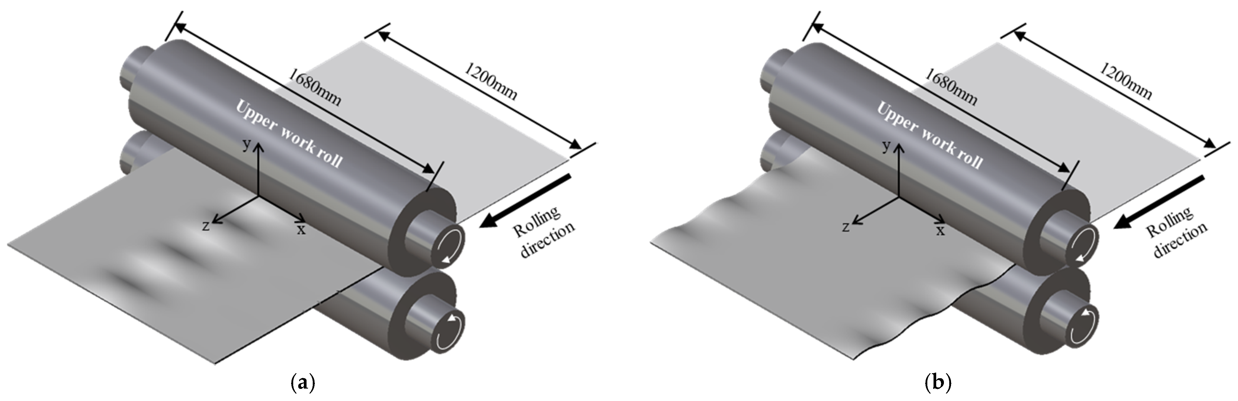
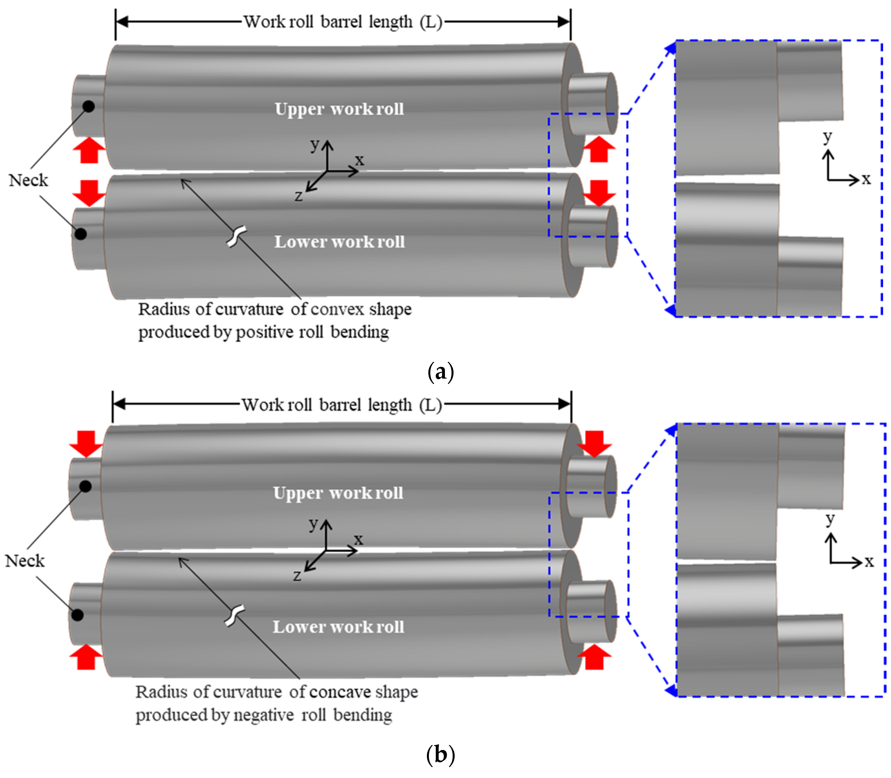
2. Description of Roll Bending

All the parts that compose a rolling mill are subjected to elastic deformation by the rolling force. The amount of deformation of the work rolls in a widthwise account for 60–70%. The bending of the work rolls results in a widthwise distribution of strip thickness in the form of a convex or concave. Therefore, the operator controls the bending of the work rolls in the width direction using hydraulic pistons [11]. Figure 2a shows a positive roll-bending profile. The red arrows indicate the force generated by the hydraulic piston is applied to the neck to control roll bending. The centers of the upper and lower work rolls are closer to each other than their edges. In contrast, Figure 2b shows a negative roll-bending profile. The edges of the upper and lower work rolls are closer to each other than the center of the upper and lower work.

If positive bending occurs, the roll-bending profile is bow tie, and the center of the strip is elongated to a greater extent in the rolling direction than in the edges [4]. In order for the strip to maintain a continuous body, the strains in the center and at the edges readjust so that the center is shortened, and the edges are elongated. Thus, compressive stresses are generated at the center and subsequently leads to a lack of flatness at the strip center (Figure 1a). At the same time, tensile stresses are generated in the strip edges, which cause local fracture on both sides in the strip. If the work rolls are bent otherwise by the hydraulic pistons, negative bending occurs. Then, the opposite phenomenon develops (Figure 1b).

3. Experiments

3.1. Specimens for Uniaxial Tensile Test

Hot-rolled 3.0 wt% silicon steel strip was machined into sheet-type specimens according to ASTM E8/E8M-16a. Figure 3 shows the dimensions of the specimen used for uniaxial tensile testing and the actual appearance of the machined specimen.

With the specimens, a uniaxial tensile test was performed to measure the stress–strain curves of 3.0 wt% high-silicon steel. The gauge length of the sheet-type specimens was 50 mm, and the thickness was 2.3 mm. The strain was converted by measuring the change in gauge length using an Instron AutoX 750(automatic extensometer). The stress–strain curves were measured at room temperature using an Instron 5982 (100 kN). The strain rate applied to the tensile test was 0.0067/s.

3.2. Specimens for Fracture Test

Figure 4a–d show the dimensions and actual photographs of the specimens with four different shapes (notched tensile with R = 10 mm (NT10), notched tensile with R = 30 mm (NT30), sharped-notch tensile (SNT), and in-plane shear (IPS)) used to construct 3D fracture loci that vary with the stress triaxialities and Lode angle parameters. Hereinafter, for convenience, the specimens of the four shapes are referred to as NT10, NT30, SNT, and IPS, respectively. All specimens were machined by electro-discharge. Fracture tests using four-eight specimens with different shapes were performed to construct the 3D fracture loci of steels (DP600 [12,13], aluminum 6451 [14], TRIP780, DP780, and DP590 [15]). Following the previous studies [12,13,14,15], this study constructed a 3D fracture locus of high-silicon steel using five different specimens (Figure 3 and Figure 4a–d).

Similar to the method that Lian et al. [13] adopted, this study measured the cross-head movement to calculate the strain because it was difficult to attach the extensometer to the specimens due to the geometry of the specimens. There was no slippage of the specimen during gripping. The specimens were tensioned past the necking point until failure.

The specimen shape in Figure 4d, proposed by Gao [16], was used to measure the equivalent strain at fracture in the in-plane shear state. Because it is difficult to attach a gauge indicator to the specimens, the displacement was measured as the movement distance of the crosshead. The cross-head speed was set to 24 mm/min.

4. Stress–Strain Behavior of High Silicon Steel

The constitutive behavior of high silicon steel is expressed in a combination of exponential form and power law form. Paredes [17] reported that the predicted stress–strain behavior after yield as well as after strain localization was consistent with measurements when the Swift model [18] and Voce model [19] were properly combined, as shown in Equation (1):

$${\overline{\sigma }}_c\left(\overline{\epsilon }\right)=\alpha \ast {\overline{\sigma }}_s\left(\overline{\epsilon }\right)+\left(1-\alpha \right)\ast {\overline{\sigma }}_v\left(\overline{\epsilon }\right),$$

(1)

$$\mathrm{where}{\overline{\sigma }}_s\left(\overline{\epsilon }\right)=A_1\ast {\left({\epsilon }_0+\overline{\epsilon }\right)}^{A_2},$$

(2)

$${\overline{\sigma }}_v\left(\overline{\epsilon }\right)=B_1+B_2\ast \left(1-exp\left(-B_3\ast \overline{\epsilon }\right)\right)$$

(3)

where $A_1$, ε₀, and$A_2$ are the material constants of the Swift model (Equation (2)), and $B_1$,$B_2,$ and $B_3$ are the material constants of the Voce model (Equation (3)). These constants were calibrated by fitting the equivalent stress (${\overline{\sigma }}^{Pred}$) predicted from Equations (2) and (3) to the measured equivalent stress (${\overline{\sigma }}^{meas}$). The calibration accuracy was assessed using the root mean squared error (RMSE) represented by Equation (4). The RMSE was 1.036 for the Swift model and 0.2835 for the Voce model, respectively.

$$RMSE=\sqrt{\frac{1}{n}{{\displaystyle \sum }}_{i=1}^n{\left({\overline{\sigma }}^{meas}-{\overline{\sigma }}^{Pred}\right)}^2}$$

(4)

Table 1. Parameters of the combined model for 3.0 wt% silicon steel.

ε0	A1 (MPa)	A2	B1 (MPa)	B2 (MPa)	B3	α
0.003552	1009	0.1485	515.5	274.9	13.75	0.7

summarizes the values of the calibrated material constants. α is a weighting factor with a value between 0 and 1. α (=0.7) was determined by comparing the global force–displacement response measured from a uniaxial tensile test with the FE simulation of the tensile test.

Figure 5a shows three equivalent stress–strain curves computed by the Swift, Voce, and combined models. The equivalent stresses and strains measured before the onset of necking are indicated by black dots. The necking point was determined by equivalent stress and strain at maximum load. It can be observed that the equivalent stress–strain curve generated by the combined model is between the curves generated by the Swift and Voce models. In this study, the equivalent stress–strain curve generated from the combined model was used in the FE analysis.

Figure 5b shows the usefulness of the combined model used in the FE analysis. The global force and displacement curves predicted from the FE simulations were compared with the measurements. The combined model predicts the global force-displacement behavior much more accurately than the other two models. It should be emphasized that the reliability of the obtained global force and displacement response is strongly correlated with the reliability of the FE simulation [20].

5. Fracture Initiation Model

It is then necessary to choose a proper fracture initiation model (ductile fracture model) that can be implemented in conjunction with the FE analysis. To date, three representative approaches incorporated with FE analysis are used for predicting the fracture of materials in the cold forming.

(i) Phenomenological continuum damage model (CDM): This approach utilizes the internal damage variable (scalar if the material is isotropic and tensor if it is anisotropic) to quantify the degree of deterioration in the material stiffness and strength during elastic–plastic deformation. This approach was first proposed by Kachanov [21] to describe the creep damage and was later extended to ductile damage in elastic–plastic deformation by Chaboche [22] and Lemaitre [23]. CDM is coupled with constitutive equations supported by thermodynamics of irreversible processes. However, CDM generally does not explicitly account for morphology and damage mechanisms in the microstructure [24] in addition, many material parameters in this model have to be identified, making them inconvenient for applications [25].

(ii) Micromechanics-based damage model (MDM). This approach uses the growth of voids in the material as an internal variable to quantify the degree of damage. McClintock et al. [26] first developed a void growth model by assuming a regular array of pre-existing cylindrical voids with elliptical cross-sections in a non-hardening material. Gurson [27] introduced a plastic potential function sensitive to porosity (i.e., the void volume fraction) and stress triaxiality so that the influence of void growth on the yield surface could be taken into account. The Gurson–Tvergaard–Needleman [28] (GTN) model that predicts ductile fracture on the basis of the nucleation, growth, and coalescence of voids in materials is most widely used. Gurson-like models are generally adequate to simulate predominate tensile fracture in moderate and high stress triaxiality conditions, but fail to predict fracture in the low and negative stress triaxiality domains [29]. However, recently, a modified GTN model [30,31] including a void shear mechanism emerged, enabling the analysis of ductile fracture behaviors under a wide range of triaxiality. Nevertheless, it is not easy to link FE analysis and MDM to produce results. For example, the GTN model has nine material parameters that need to be calibrated.

(iii) Uncoupled phenomenological ductile fracture model (DFM): This approach does not employ directly an internal variable to depict the damage. This approach introduces so-called the damage indicator w, the cumulative equivalent strain up to fracture. A point in the material (or an element in FE analysis) is assumed to fracture if the value of w reaches a material dependent critical value, which can be obtained by performing fracture tests with specimens of various shapes and FE analyses of the tests. A feature of the above mentioned CDM and MDM is that the progressive deterioration of the material is implicitly embedded in the formulation of the constitutive equations (i.e., coupled approach). Meanwhile, the ductile fracture criterion has no influence on the state of constitutive equation, that is, there is no coupling between damage and the formulation of the constitutive equations. However, DFM has fewer material parameters that need to be calibrated and has proven to be able to simulate the fracture initiation of material with acceptable engineering accuracy [32,33,34,35]. Hence, the uncoupled approach is adopted in the present study.

DFM assumes that fracture of elastic-plastic solids begins when the cumulative damage within the material reaches a threshold. The accumulated damage is called the damage indicator w and is expressed as follows.

$$w={{\displaystyle \int }}_0^{{\overline{\epsilon }}_f}\frac{d\overline{\epsilon }}{{\overline{\epsilon }}_f\left(\eta ,\overline{\theta }\right)}$$

(5)

Here, w increases with plastic deformation, which is proportional to the incremental change in the equivalent strain. The fracture was initiated when w = 1.0. ${\overline{\epsilon }}_f\left(\eta ,\overline{\theta }\right)$ denotes the equivalent strain at fracture on an element (material point). η and $\overline{\theta }$ represent stress triaxiality and Lode angle parameter.

$$\eta =\frac{{\sigma }_m}{\overline{\sigma }}=\frac{{\sigma }_1+{\sigma }_2+{\sigma }_3}{3\overline{\sigma }}$$

(6)

$$\overline{\theta }=-\frac{2{\sigma }_2-{\sigma }_1-{\sigma }_3}{{\sigma }_1-{\sigma }_3}$$

(7)

where ${\sigma }_1$, ${\sigma }_2$ and ${\sigma }_3$ denote principal stresses. ${\sigma }_m\left(=\frac{{\sigma }_1+{\sigma }_2+{\sigma }_3}{3}\right)$ and $\overline{\sigma }$ are the mean stress and equivalent stress. As ${\overline{\epsilon }}_f\left(\eta ,\overline{\theta }\right)$ is expressed as a function of η and $\overline{\theta }$, it is plotted in the form of a surface. This surface is called the 3D fracture locus or envelope. In the actual rolling process, if residual stress remains in the strip by the previous process, a higher stress state may be obtained by the residual stress around the crack tip [36,37].

5.1. 3D Fracture Locus

Stress triaxiality is a major factor that typically affects fracture [26,27,28,38]. In particular, under high stress triaxiality conditions such as tension tests, this has a full effect on fracture. In the tension test, various stress triaxiality conditions are realized by varying the specimen shape and the notch shape, and the corresponding strain-to-fracture initiation and physical properties are then evaluated. Sajid and Kiran [39,40] evaluated the yield strength and ultimate tensile strength of structural steels for each tension specimen shape and examined their dependence on stress triaxiality. Kang et al. [41] calibrated a two-parameter ductile fracture model through tension test and FE analysis for stress triaxiality due to various notch changes in tensile specimens. Unlike the tension test, since the range of stress triaxiality in rolling is −1.2 to 1.2 [8], the effect on fracture is affected not only by stress triaxiality but also by the Lode parameter [42,43]. Therefore, a ductile fracture criterion that reflects the Lode parameter is required, and related models [10,29,34,44] are the maximum shear model [44], the modified Mohr–Coulomb (MMC) fracture criterion [10] and so on. In this study, the MMC model, which can predict fracture well not only at high triaxiality but also at negative and low triaxiality, was adopted.

Bai and Wierzbicki [10] proposed the modified Mohr–Coulomb (MMC) criterion (model) to predict the ductile fracture of 2024-T531 aluminum and TRIP690 materials during the cold forming process. Using the MMC criterion, Talebi-Ghadikolaee et al. [45] constructed the fracture locus of AA6061-T6 and predicted the fracture occurring during the forming of multi-pass rolls through FE analysis. Saneian et al. [46] predicted fracture behavior during the installation and operation of an offshore pipeline made of X80 steel subjected to tension and torsion using the MMC criterion.

${\overline{\epsilon }}_f\left(\eta ,\overline{\theta }\right)$ in the MMC criterion is expressed as follows.

$${\overline{\epsilon }}_f\left(\eta ,\overline{\theta }\right)={\left\{\begin{array}{c}\frac{K}{C_2}\left[1-C_{\eta }\left(\eta -{\eta }_0\right)\right]\times \left[C_{\theta }^s+\frac{\sqrt{3}}{2-\sqrt{3}}\left(C_{\theta }^{ax}-C_{\theta }^s\right)\left(\sec \left(\frac{\pi \overline{\theta }}{6}\right)-1\right)\right]\\ \times \left[\sqrt{\frac{1+C_1{}^2}{3}}\cos \left(\frac{\pi \overline{\theta }}{6}\right)+C_1\left(\eta +\frac{1}{3}\sin \left(\frac{\pi \overline{\theta }}{6}\right)-1\right)\right]\end{array}\right\}}^{-\frac{1}{n}}$$

(8)

Equation (8) was adopted in this study to simulate the edge cracking of a strip during cold rolling. The eight parameters (K, n, ${\mathrm{C}}_{\eta }$, ${\eta }_0$, $C_{\theta }^s$, $C_{\theta }^{ax}$, $C_1$, and $C_2$) must be calibrated for the construction of the fracture envelope from the MMC criterion. K and n are the same material constants adjusted for the power law ($\overline{\sigma }$=$K{\overline{\epsilon }}^n$) [17]. ${\mathrm{C}}_{\eta }$ and ${\eta }_0$ are the parameters that determine the yield criterion. The dependence of the Lode angle parameter is controlled by $C_{\theta }^s$, and the asymmetry of the fracture locus is influenced by the parameter $C_{\theta }^{ax}$. The constants $C_1$ and $C_2$ must be determined through fracture tests. Because the von Mises yield function was used in this study, $C_{\eta }$ = 0 and $C_{\theta }^s$ = $C_{\theta }^{ax}$ = 1 [34]. Therefore, Equation (8) can be expressed as follows:

$${\overline{\epsilon }}_f\left(\eta ,\overline{\theta }\right)={\left\{\frac{K}{C_2}\times \left[\sqrt{\frac{1+C_1{}^2}{3}}\cos \left(\frac{\pi \overline{\theta }}{6}\right)+C_1\left(\eta +\frac{1}{3}\sin \left(\frac{\pi \overline{\theta }}{6}\right)-1\right)\right]\right\}}^{-\frac{1}{n}}$$

(9)

As the stress state varied within a small range during the plastic deformation of each specimen, the averaged stress triaxiality, ${\eta }_{avg}\left(=\frac{1}{{\overline{\epsilon }}_f}{{\displaystyle \int }}_0^{{\overline{\epsilon }}_f}\eta \left(\overline{\epsilon }\right)d\overline{\epsilon }\right)$, and the averaged Lode angle parameter, ${\overline{\theta }}_{avg}\left(=\frac{1}{{\overline{\epsilon }}_f}{{\displaystyle \int }}_0^{{\overline{\epsilon }}_f}\overline{\theta }\left(\overline{\epsilon }\right)d\overline{\epsilon }\right)$, were utilized to determine the parameters $\left(\eta ,\overline{\theta }\right)$ [20]. In this study, the element removing method [47,48] is used to simulate crack growth. Hence, the material stiffness of the element where fracture has begun should be gradually reduced.

5.2. Material Stiffness Degradation

Once a fracture initiates for any element, the material stiffness at that element is gradually reduced until it reaches zero. If the material stiffness is suddenly reduced to zero, numerical instability occurs. This is because ${\overline{\epsilon }}_f$ depends on the mesh size. This mesh dependency is overcome by replacing the softening part of the equivalent stress–strain curve with the equivalent stress ($\overline{\sigma }$)-equivalent plastic displacement (${\overline{u}}^p)$ curve after fracture initiation. The implementation of the relation $\overline{\sigma }–{\overline{u}}^p$ in the FE analysis is described in Abaqus [48]. The equivalent plastic displacement rate at an element is expressed as follows:

$${\dot{\overline{u}}}^p=L_e\dot{\overline{\epsilon }}$$

(10)

L_e, depending on the element geometry, indicates the characteristic length of the element. The definition of L_e associated with an integration point is necessary to stabilize the FE analysis.

In this manner, a crack initiates at an element in the material (strip), the material stiffness at that element is gradually degraded, and the element completely loses its load-carrying capacity. If these sequences are repeated on adjacent elements and in arbitrary directions, crack propagation in arbitrary directions is simulated.

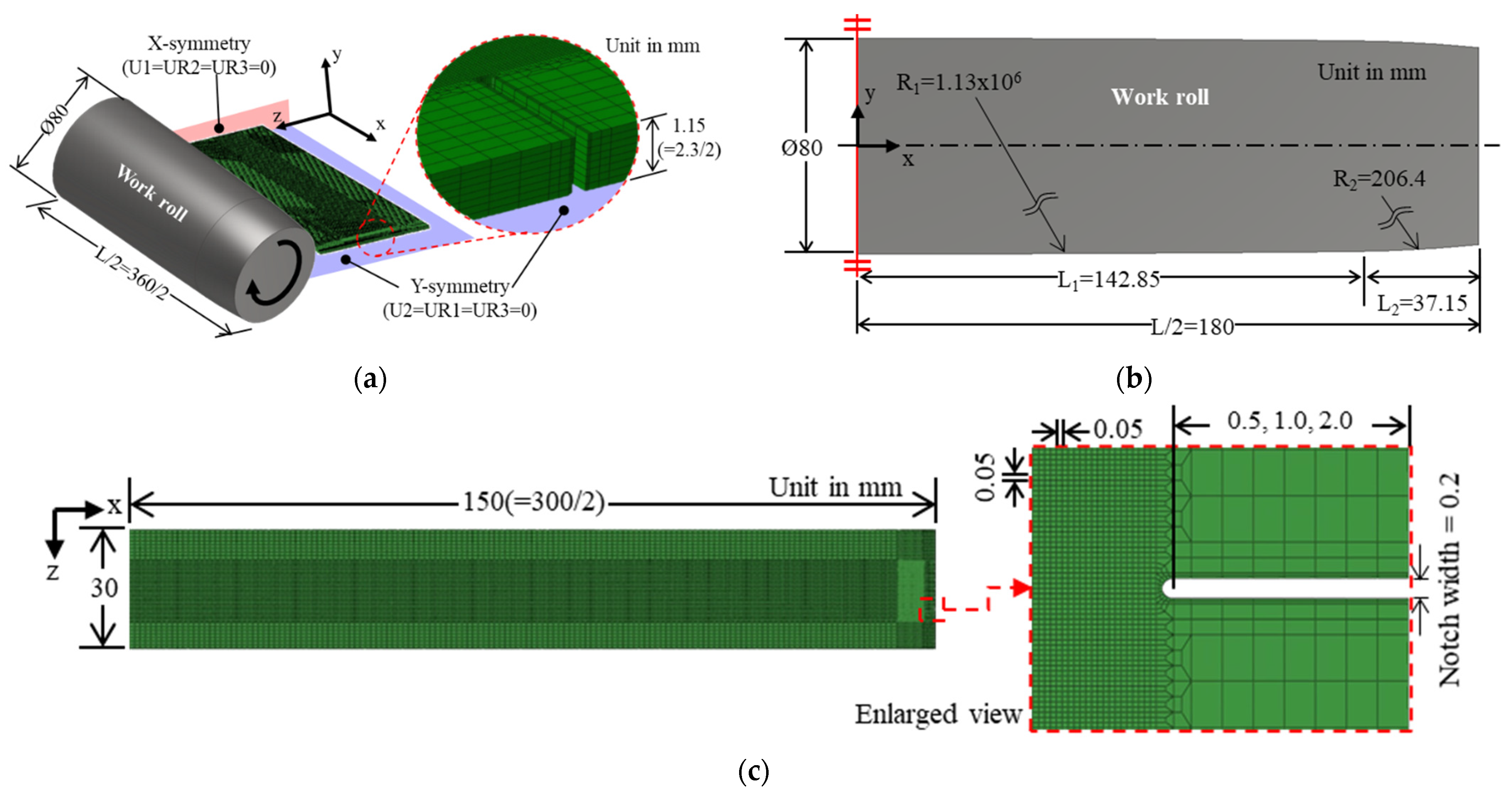
6. FE Simulation of Cold Rolling

FE analyses with the von Mises plasticity were carried out using Abaqus/Explicit [48]. The constitutive equation and MMC DF criterion were implemented into a VUMAT user-defined subroutine. In this paper, the material is assumed to be isotropic. A quarter model was used to shorten the runtime.

Figure 6a shows a half symmetric model of work roll and a quarter symmetric model of strip and boundary conditions. The work roll with positive roll bending curvature was modeled as analytically rigid. The rolling speed was 400 mm/s. Coulomb friction condition (τ = μ${\sigma }_n$) was used at the interface of the work roll and strip.

Figure 6b illustrates the dimensions of the half symmetrical model of work roll barrel that mimics positive roll bending. The barrel length ratio (L₂/L₁) was fixed at 0.26 based on the process data of the actual cold rolling mill. Hence, the main radius of curvature R₁ was set to 1.13 × 10⁶ mm and the secondary radius of curvature R₂ was set to 206.4 mm. The variables that directly affect edge cracking are L₂ and R₂.

In Figure 6c, the 300 mm wide and 2.3 mm thick strip was meshed with an eight-node reduced integration brick element (C3D8R) to reduce computation time. Yan et al. [5] performed optical imaging analysis on the edges of hot-rolled silicon strip. They showed that there was a notch-like crack at the edge of the strip; the notch length was about 0.5–1.5 mm, and the notch tip diameter was about 0.2 mm. Therefore, in this study, the notch tip diameter was fixed at 0.2 mm and the notch lengths were set to 0.5, 1.0, and 2.0 mm, respectively. The elastic modulus of the strip was 190 GPa, the density was 7650 kg/m³, and Poisson’s ratio was 0.3.

Byon et al. [8] showed that the pilot cold rolling test and FE analysis results were consistent when the element size in the x and z-directions around the notch tip of high silicon steel strip was 0.05 mm, respectively. Hence, mesh convergence test in this study was performed to determine the appropriate number of elements in the strip thickness direction.

Table 2. Variations in the equivalent strain at the fracture as number of elements in the thickness direction of the strip changes.

No. of Elements	2	4	6	8	10
Equivalent strain at fracture	0.5962	0.5844	0.5786	0.5767	0.5770

shows that FE mesh may have eight elements in the thickness direction of the strip to ensure the convergence of the equivalent strain at the fracture. Therefore, refined mesh size in the vicinity of notches is 0.05 mm × 0.14 mm (≈2.3/8 mm) × 0.05 mm. Total 151,629 elements were used.

The automatic mass scaling (AMS) technique was applied to the entire model to further reduce runtime [49]. There are three parameters of AMS, namely feed rate, extruded element length, and nodes in cross-section; values of 400 mm/s, 0.05 mm, and 2156 ea were used, respectively, for these parameters. The mass scale was updated every 100 time increments.

7. Results and Discussion

7.1. Force, Displacement, and Equivalent Strain Responses in Different Stress States

In Figure 7, the global forces measured by the fracture tests using specimens of four different shapes are shown. In addition, the global forces and equivalent strains predicted by the FE analysis of the fracture tests are also shown. Strain localization prior to ductile fracture accompanied by necking was observed during the fracture tests. The black dashed line indicates the position where strain localization (hereafter referred to as SL) occurred. In each figure, the global forces (measured vs. predicted) are compared first, and variations in the equivalent strain are explained later.

In Figure 7a, the predicted and measured forces are in good agreement when the NT10 specimen is used. Similar to the uniaxial tensile test with the standard (dog bone) tensile specimen (Figure 5b), the force gradually decreased after SL. This confirms that the combined model [15] used in the FE analysis is appropriate.

A softening of the flow curve (from SL to the onset of fracture) was observed. This is attributed to the fact that even though ${\eta }_{avg}$ is high (0.5349), the absolute value of ${\overline{\theta }}_{avg}$ is relatively low (0.4551). Hence, the onset of fracture due to the shearing of the voids was delayed. Note that the smaller the Lode angle parameter, the faster is the occurrence of the fracture due to void shear. The calculated values of ${\eta }_{avg}$, ${\overline{\theta }}_{avg}$, and ${\overline{\epsilon }}_f$ are summarized in

Table 3. Loading parameters and equivalent strain at fracture for different types of specimens.

Specimen Type	${\mathit{\eta }}_{\mathit{a}\mathit{v}\mathit{g}}$	${\overline{\mathit{\theta }}}_{\mathit{a}\mathit{v}\mathit{g}}$	${\overline{\mathit{\epsilon }}}_{\mathit{f}}$
Standard (dog-bone)	0.4424	0.7366	0.7893
NT10	0.5349	0.4551	0.5416
NT30	0.4916	0.6145	0.6755
SNT	0.8301	0.2235	0.2116
IPS	0.0118	0.0305	1.0993

. The magnitude of ${\eta }_{avg}$ is generally classified as follows: 0 or less, low; 0–1/3, moderate; 1/3–2/3, high; 2/3 or more, very high. However, there is no classification of the magnitude of the Lode angle parameter.

Figure 7b shows that as the notch radius of the NT30 specimen is large, more deformation (longer cross head displacement) is required until the specimen reaches fracture after SL. The predictions and measurements are very similar, which means that the selection of the combined model is appropriate. As with the NT10 specimen, softening was observed for the NT30 specimen. Considering the product of $\eta$ and $\overline{\theta }$ values of two specimens (NT10 and NT30) as a measure trade-off, the reason for the softening is explained.

In the SNT specimen (Figure 7c), unlike in the specimens with large notch radii such as NT10 and NT30, SL and fracture occur almost simultaneously. This is explained as follows: when $\eta$ is very high, the strain to localization decreases because of the void growth [50,51]. However, if the absolute value of $\overline{\theta }$ is small, fracture occurs more rapidly by shearing of the voids, and therefore, little softening is observed [52]. For the SNT specimen, $\eta$ is as very high as 0.8301, but $\overline{\theta }$ is as small as 0.2235.

In Figure 7d, the IPS and SNT specimens are similar in that softening is hardly observed owing to rapid fracture. However, the IPS specimen can withstand approximately 12 times greater displacement than the SNT specimen until the onset of fracture. In the case of the IPS specimen, fracture by shearing of voids occurs because $\overline{\theta }$ is also very small (0.0305), even though $\eta$is close to zero (0.0118).

In addition, Figure 7a–d indicate that the profile of the increasing equivalent strain $\overline{\epsilon }$ is also slightly different across specimens, because the stress states in each specimen are different. However, except for IPS specimen, $\overline{\epsilon }$ computed at the center (marked with a black dot) of the specimen cross-section monotonically increases with the displacement. ${\overline{\epsilon }}_f$ in Figure 7c was very small (0.2116) because the notch effect accelerating the onset of fracture was significant. In contrast, ${\overline{\epsilon }}_f$ in Figure 7d is large (1.0993) because the IPS specimen fractured by almost pure shear strain.

In summary, the analysis of SL and onset of fracture demonstrate that the MMC criterion adopted in this study is reasonable for predicting crack initiation, and subsequently, propagation, in the 3.0 wt% silicon steel strip.

7.2. Fracture Locus

Four parameters of the MMC criterion (K, n, C₁, C₂) in Equation (9) were calibrated to generate a 3D fracture locus. Matlab2021-a was used for calibration. K and n were calibrated by fitting the data measured in the uniaxial tensile test to the curve generated from the power law. C₁ and C₂ were calibrated using least-squares optimization. These approaches minimize the cumulative error between the constructed 3D fracture locus and the measured data. The calibrated values are listed in

Table 4. Parameters used in the MMC fracture locus (3D).

K (MPa)	n	${\mathit{C}}_1$	${\mathit{C}}_2$
976.2	0.1299	0.1226	558.7

. The optimized mean squared error (MSE) was 0.04476.

$$MSE=\frac{1}{n}{{\displaystyle \sum }}_{i=1}^n{\left({\overline{\epsilon }}_f^{FEA}-{\overline{\epsilon }}_f\right)}^2$$

(11)

In Equation (11), ${\overline{\epsilon }}_f^{FEA}$ is the equivalent strain at fracture computed from the FE analysis. ${\overline{\epsilon }}_f$ is the equivalent strain at the fracture obtained from the 3D fracture locus. ‘n’ denotes the number of specimens used for uniaxial tensile and fracture tests. The 3D fracture surface constructed in this manner is shown in Figure 8a.

For comparative purposes, a 2D fracture using the Johnson–Cook (J–C) fracture criterion [9] was also constructed. The J–C fracture criterion is expressed as follows:

$${\overline{\epsilon }}_f\left(\eta \right)=d_1+d_{2}exp\left(-d_3\ast \eta \right)$$

(12)

The parameters (d₁, d₂, and d₃) were calibrated in the manner mentioned above. The calibrated values are listed in

Table 5. Parameters used in the J–C fracture locus (2D).

${\mathit{d}}_1$	${\mathit{d}}_2$	${\mathit{d}}_3$
0.08478	5.133	4.467

. The optimized mean squared error (MSE) was only 0.02494. Figure 8b shows the J–C fracture locus (2D). As shown, the J–C fracture locus is applicable when predicting the fracture of materials at high and very high stress triaxialities.

7.3. Numerical Analysis of Edge Cracking in the Strip

Figure 9a,b show the difference in edge cracking when 2D and 3D fracture loci are used. The thickness reduction ratio was 25%, the initial notch length was 2 mm, and the secondary radius of curvature of the work roll surface profile (positive roll bending) was 206.4 mm. The tip of the notch was enlarged to observe edge cracking in detail. The length of crack growth in the transverse direction and the length of crack growth in the rolling direction are indicated by “LCGT” and “LCGR”, respectively. The direction in which the crack grew is indicated by “CGD”.

Figure 9a shows the edge cracking behavior when the 2D fracture locus (J–C criterion) was used. LCGT and LCGR are 2.09 mm and 1.73 mm, respectively. CGD is 43.68°. The crack grows in the rolling direction and then advances in the reverse rolling direction (refer to the ellipse indicated by the yellow dashed line in Figure 9a). This is because ${\overline{\epsilon }}_f$ at the advancing crack tip was computed as a function of only the stress triaxiality.

Figure 9b shows the edge cracking behavior when the 3D fracture locus (MMC criterion) was used. The LCGT and LCGR were 1.67 mm and 1.53 mm, respectively. CGD was 45.9°. The 2D fracture locus overestimates LCGT and LCGR by 20.1% and 11.6% more than the 3D fracture locus, respectively. This is because the ${\overline{\epsilon }}_f$ in the 3D fracture locus in high stress triaxialities is also influenced by variations in the Lode angle parameters.

Figure 9c shows the history of stress triaxialities (solid squares) from the point at which deformation begins at the notch tip of the strip until the onset of fracture during rolling. The Lode angle parameter $\overline{\theta }$ varied from −0.81 to 0.72. The dashed line represents the plane stress condition (${\sigma }_3$ = 0). Because the stress triaxialities (solid squares) are above the plane stress condition (dashed line), the edge cracks initiate faster with the 2D locus than with the 3D locus. ① indicates the point at which damage begins to be accumulated. ⑦ specifies the point at which fracture starts at the tip of the notch. ②–⑥ indicates the changes in the stress states at the notch tip when the strip is deformed by cold rolling.

Figure 10 shows the effect of the secondary roll-bending ratio (L₂/R₂) on the edge cracking behavior when the thickness reduction ratio of a strip for one pass was 25%. L₂ is the secondary length of the work roll barrel, and R₂ is the secondary radius of curvature of the convex profile of the work roll barrel (Figure 6), which emulates positive roll bending. Figure 10a shows that LCGT and LCGR are 1.67 mm and 1.53 mm, respectively, when L₂/R₂ is 0.18. Figure 10b illustrates that LCGT and LCGR are 0.48 mm and 0.73 mm, respectively, when L₂/R₂ is 0.09. Comparing the two cases, LCGT decreased by 71.2% and LCGR by 52.3%. This is because the tensile stress applied to the edge of the strip significantly reduced as R₂ doubled. Figure 10c shows no edge cracking when (L₁/R₁) and (L₂/R₂) are 0, which corresponds to flat rolling and is a special case. Because the profile of the work roll barrel is perfectly flat, tensile stress is scarcely applied to the strip edge, which suppresses crack initiation at the notch tip. Note that flat rolling is a condition in which actual cold rolling is almost impossible.

Figure 11 shows variations in the length of crack grown in the transverse (LCGT) direction of the strip when the R₂ and initial notch length changes at the thickness reduction ratio of 25% for a pass. LCGT reduces nonlinearly as the secondary roll-bending ratio (L₂/R₂) decreases.

The shorter the initial notch length, the smaller the crack growth. For example, when the ratio L₂/R₂ is 0.15, the LCGT corresponding to the initial notch lengths of 2 mm, 1 mm, and 0.5 mm are 1.23 mm, 1.17 mm, and 0.8 mm, respectively. This indicates that the crack growth is reduced by approximately 35% when the initial notch length is decreased from 2.0 mm to 0.5 mm. That is, if the initial crack length generating at the strip edge through trimming process after hot rolling is about 0.5 mm, the crack length growing at the strip edge during the cold rolling process can be reduced by approximately 35%. The effect of the initial notch length on the crack length grown at the edge of the strip during cold rolling is greatest when the secondary roll-bending ratio (L₂/R₂) is 0.12.

8. Application

The practical applicability of this study is likely as follows. Figure 11 shows the relationship between the magnitude of L₂/R₂ and the crack growth length, which varies with the initial crack (or notch) length. Looking at Figure 11 in reverse, it is possible for the operator of the actual cold rolling mill to measure the crack length grown after cold rolling and to guess the size of the initial crack length created on the side of the strip by trimming after hot rolling. Note that as high-silicon steel lacks ductility, cracks (or notches) with a length of 0.5 to 1 mm can be generated at any time in the trimming process after hot rolling. The operators may adjust the appropriate magnitude of L₂/R₂ for controlling the length of crack growing during cold rolling to be below the target value.

9. Concluding Remarks

In this study, 2D and 3D fracture loci of high-silicon steel strips were constructed by performing uniaxial tensile tests with standard tensile specimens and fracture tests using four different specimen shapes. The developed 3D fracture locus was implemented into a VUMAT user-defined subroutine of Abaqus. A series of FE analyses coupled with the 3D fracture locus was performed to interpret edge cracking in the strip as the secondary roll-bending ratio (L₂/R₂) changes. The difference between the 3D and 2D fracture loci was also analyzed through an FE simulation of edge cracking. The conclusions are as follows.

1.

The 2D fracture locus at a high triaxiality of 13.1–22.2% overestimates the edge cracking. Therefore, edge cracking should be predicted using the 3D fracture locus that includes stress triaxiality, and Lode angle parameters varying between −0.81and 0.71 should be used.

2.

As the initial notch length at the edges of the trimmed strip after hot rolling is shortened, the length of crack grown in the transverse direction at the edge of the strip was reduced non-linearly. This effect was greatest when the secondary roll-bending ratio was 0.12.

References

1. Hilbert, H.G.; Roemmen, H.J.; Boucke, K.E. MKW cold mill rolling silicon steel strip. Iron Steel Eng. 1976, 25, 25–31. [Google Scholar]
2. Chen, A.-H.; Guo, H.-R.; Li, H.-L.; Emi, T. Formation of edge crack in 1.4% Si non-oriented electrical steel during hot rolling. J. Iron Steel Res. Int. 2014, 21, 269–274. [Google Scholar] [CrossRef]
3. Lee, S.H.; Lee, K.H.; Lee, S.B.; Kim, B.M. Study of edge-cracking characteristics during thin-foil rolling of Cu-Fe-P strip. Int. J. Precis. Eng. Manuf. 2013, 14, 2109–2118. [Google Scholar] [CrossRef]
4. Byon, S.M.; Lee, Y. Experimental study on the prohibition of edge cracking of high-silicon steel strips during cold rolling. Proc. Inst. Mech. Eng. Part B J. Eng. Manuf. 2011, 225, 1983–1988. [Google Scholar] [CrossRef]
5. Yan, Y.; Sun, Q.; Chen, J.; Pan, H. The initiation and propagation of edge cracks of silicon steel during tandem cold rolling process based on the Gurson-Tvergaard-Needleman damage model. J. Mater. Process. Technol. 2013, 213, 598–605. [Google Scholar] [CrossRef]
6. Tvergaard, V.; Needleman, A. Analysis of the cup-cone fracture in a round tensile bar. Acta Metall. 1984, 32, 157–169. [Google Scholar] [CrossRef]
7. Sun, Q.; Chen, J.; Pan, H. Prediction of edge crack in cold rolling of silicon steel strip based on an extended Gurson-Tvergaard-Needleman damage model. J. Manuf. Sci. Eng. Trans. ASME 2015, 137, 1–6. [Google Scholar] [CrossRef]
8. Byon, S.M.; Roh, Y.H.; Yang, Z.; Lee, Y. A roll-bending approach to suppress the edge cracking of silicon steel in the cold rolling process. Proc. Inst. Mech. Eng. Part B J. Eng. Manuf. 2021, 235, 112–124. [Google Scholar] [CrossRef]
9. Johnson, G.R.; Cook, W.H. Fracture characteristics of three metals subjected to various strains, strain rates, temperatures and pressures. Eng. Fract. Mech. 1985, 21, 31–48. [Google Scholar] [CrossRef]
10. Bai, Y.; Wierzbicki, T. Application of extended Mohr—Coulomb criterion to ductile fracture. Int. J. Fract. 2010, 161, 1–20. [Google Scholar] [CrossRef]
11. JFE Deformation of Rolling Mill. Available online: http://www.jfe-21st-cf.or.jp/chapter_3/3b_2.html (accessed on 7 August 2021).
12. Qin, S.; Beese, A.M. Multiaxial fracture of DP600: Experiments and finite element modeling. Mater. Sci. Eng. A 2020, 785, 139386. [Google Scholar] [CrossRef]
13. Lian, J.; Sharaf, M.; Archie, F.; Münstermann, S. A hybrid approach for modelling of plasticity and failure behaviour of advanced high-strength steel sheets. Int. J. Damage Mech. 2013, 22, 188–218. [Google Scholar] [CrossRef]
14. Abi-Akl, R.; Mohr, D. Paint-bake effect on the plasticity and fracture of pre-strained aluminum 6451 sheets. Int. J. Mech. Sci. 2017, 124–125, 68–82. [Google Scholar] [CrossRef] [Green Version]
15. Mohr, D.; Marcadet, S.J. Micromechanically-motivated phenomenological Hosford-Coulomb model for predicting ductile fracture initiation at low stress triaxialities. Int. J. Solids Struct. 2015, 67–68, 40–55. [Google Scholar] [CrossRef]
16. Gao, F.; Gui, L.; Fan, Z. Experimental and Numerical Analysis of an In-Plane Shear Specimen Designed for Ductile Fracture Studies. Exp. Mech. 2011, 51, 891–901. [Google Scholar] [CrossRef]
17. Paredes, M.; Lian, J.; Wierzbicki, T.; Cristea, M.E.; Münstermann, S.; Darcis, P. Modeling of plasticity and fracture behavior of X65 steels: Seam weld and seamless pipes. Int. J. Fract. 2018, 213, 17–36. [Google Scholar] [CrossRef]
18. Swift, H.W. Plastic instability under plane stress. J. Mech. Phys. Solids 1952, 1, 1–18. [Google Scholar] [CrossRef]
19. Voce, E. The relationship between stress and strain for homogeneous deformation. J. Inst. Met. 1948, 74, 537–562. [Google Scholar]
20. Mu, L.; Zang, Y.; Wang, Y.; Li, X.L.; Araujo Stemler, P.M. Phenomenological uncoupled ductile fracture model considering different void deformation modes for sheet metal forming. Int. J. Mech. Sci. 2018, 141, 408–423. [Google Scholar] [CrossRef]
21. Kachanov, L.M. On creep rupture time. Izv. Acad. Nauk SSSR Otd. Techn. Nauk 1958, 8, 26–31. [Google Scholar]
22. Chaboche, J.L. Anisotropic creep damage in the framework of continuum damage mechanics. Nucl. Eng. Des. 1984, 79, 309–319. [Google Scholar] [CrossRef] [Green Version]
23. Lemaitre, J. Local approach of fracture. Eng. Fract. Mech. 1986, 25, 523–537. [Google Scholar] [CrossRef]
24. Zhang, X.; O’Brien, D.J.; Ghosh, S. Parametrically homogenized continuum damage mechanics (PHCDM) models for composites from micromechanical analysis. Comput. Methods Appl. Mech. Eng. 2019, 346, 456–485. [Google Scholar] [CrossRef]
25. Li, H.; Wang, J.; Wang, J.; Hu, M.; Peng, Y. Continuum Damage Mechanics Approach for Modeling Cumulative-Damage Model. Math. Probl. Eng. 2021, 1–12. [Google Scholar] [CrossRef]
26. McClintock, F.A.; Kaplan, S.M.; Berg, C.A. Ductile fracture by hole growth in shear bands. Int. J. Fract. Mech. 1966, 2, 614–627. [Google Scholar] [CrossRef]
27. Gruson, A.L. Continuum theory of ductile rupture by void nucleation and growth: Part I-Yield criteria and flow rules for porous ductile media. J. Eng. Mater. Technol. 1977, 99, 2–15. [Google Scholar] [CrossRef]
28. Needleman, A.; Tvergaard, V.F. An analysis of ductile rupture in notched bars. J. Mech. Phys. Solids 1984, 32, 461–490. [Google Scholar] [CrossRef]
29. Wen, H.; Mahmoud, H. New Model for Ductile Fracture of Metal Alloys. I: Monotonic Loading. J. Eng. Mech. 2016, 142, 04015088. [Google Scholar] [CrossRef]
30. Jiang, W.; Li, Y.; Su, J. Modified GTN model for a broad range of stress states and application to ductile fracture. Eur. J. Mech. A/Solids 2016, 57, 132–148. [Google Scholar] [CrossRef]
31. Zhu, Y.; Engelhardt, M.D. Prediction of ductile fracture for metal alloys using a shear modified void growth model. Eng. Fract. Mech. 2018, 190, 491–513. [Google Scholar] [CrossRef]
32. Cockcroft, M.G.; Latham, D.J. Ductility and the Workability of Metals. J. Inst. Met. 1968, 96, 33–39. [Google Scholar]
33. Oyane, M.; Sato, T.; Okimoto, K.; Shima, S. Criteria for ductile fracture and their applications. J. Mech. Work. Technol. 1980, 4, 65–81. [Google Scholar] [CrossRef]
34. Bai, Y.; Wierzbicki, T. A new model of metal plasticity and fracture with pressure and Lode dependence. Int. J. Plast. 2008, 24, 1071–1096. [Google Scholar] [CrossRef]
35. Lou, Y.; Huh, H.; Lim, S.; Pack, K. New ductile fracture criterion for prediction of fracture forming limit diagrams of sheet metals. Int. J. Solids Struct. 2012, 49, 3605–3615. [Google Scholar] [CrossRef] [Green Version]
36. Fratini, L.; Macaluso, G.; Pasta, S. Residual stresses and FCP prediction in FSW through a continuous FE model. J. Mater. Process. Technol. 2009, 209, 5465–5474. [Google Scholar] [CrossRef]
37. Marannano, G.V.; Mistretta, L.; Cirello, A.; Pasta, S. Crack growth analysis at adhesive-adherent interface in bonded joints under mixed mode I/II. Eng. Fract. Mech. 2008, 75, 5122–5133. [Google Scholar] [CrossRef]
38. Rice, J.R.; Tracey, D.M. On the ductile enlargement of voids in triaxial stress fields*. J. Mech. Phys. Solids 1969, 17, 201–217. [Google Scholar] [CrossRef] [Green Version]
39. Sajid, H.U.; Kiran, R. Influence of high stress triaxiality on mechanical strength of ASTM A36, ASTM A572 and ASTM A992 steels. Constr. Build. Mater. 2018, 176, 129–134. [Google Scholar] [CrossRef]
40. Sajid, H.U.; Kiran, R. Post-fire mechanical behavior of ASTM A572 steels subjected to high stress triaxialities. Eng. Struct. 2019, 191, 323–342. [Google Scholar] [CrossRef]
41. Kang, L.; Ge, H.; Fang, X. An improved ductile fracture model for structural steels considering effect of high stress triaxiality. Constr. Build. Mater. 2016, 115, 634–650. [Google Scholar] [CrossRef]
42. Bao, Y. Prediction of Ductile Crack Formation in Uncracked Bodies. Ph.D. Thesis, Massachusetts Institute of Technology, Cambridge, MA, USA, 2003. [Google Scholar]
43. Bao, Y.; Wierzbicki, T. On fracture locus in the equivalent strain and stress triaxiality space. Int. J. Mech. Sci. 2004, 46, 81–98. [Google Scholar] [CrossRef]
44. Wierzbicki, T.; Bao, Y.; Lee, Y.W.; Bai, Y. Calibration and evaluation of seven fracture models. Int. J. Mech. Sci. 2005, 47, 719–743. [Google Scholar] [CrossRef]
45. Talebi-Ghadikolaee, H.; Naeini, H.M.; Mirnia, M.J.; Mirzai, M.A.; Alexandrov, S.; Zeinali, M.S. Modeling of ductile damage evolution in roll forming of U-channel sections. J. Mater. Process. Technol. 2020, 283, 116690. [Google Scholar] [CrossRef]
46. Saneian, M.; Han, P.; Jin, S.; Bai, Y. Fracture response of steel pipelines under combined tension and torsion. Thin-Walled Struct. 2020, 154, 106870. [Google Scholar] [CrossRef]
47. Hillerborg, A.; Modéer, M.; Petersson, P.-E. Analysis of crack formation and crack growth in concrete by means of fracture mechanics and finite elements. Cem. Concr. Res. 1976, 6, 773–781. [Google Scholar] [CrossRef]
48. Manual, A.U. Abaqus Theory Guide; Version 6.14; USA Dassault Systemes Simulia Corp: Johnston, RI, USA, 2014. [Google Scholar]
49. Documentation, A.U. Abaqus Documentation; Version 6.14; USA Dassault Systemes Simulia Corp: Johnston, RI, USA, 2014. [Google Scholar]
50. Gao, X.; Zhang, G.; Roe, C. A study on the effect of the stress state on ductile fracture. Int. J. Damage Mech. 2010, 19, 75–94. [Google Scholar] [CrossRef]
51. Cao, T.S. Models for ductile damage and fracture prediction in cold bulk metal forming processes: A review. Int. J. Mater. Form. 2017, 10, 139–171. [Google Scholar] [CrossRef]
52. Liu, W.; Lian, J.; Münstermann, S. Damage mechanism analysis of a high-strength dual-phase steel sheet with optimized fracture samples for various stress states and loading rates. Eng. Fail. Anal. 2019, 106, 104138. [Google Scholar] [CrossRef]
Figure 1. Scheme of change in the cross section of the strip due to roll bending. (a) Central wrinkle (center buckle) by positive roll bending; (b) Edge waviness by negative roll bending.
Applsci 11 08408 g001
Figure 2. Schematic of two types of roll bending. (a) Positive roll bending (b) Negative roll bending.
Applsci 11 08408 g002
Figure 3. Tensile specimen used to measure equivalent stress–strain behavior of 3.0 wt% silicon steel.
Applsci 11 08408 g003
Figure 4. Types of specimens used for constructing 3D fracture locus of 3.0 wt% silicon steel: (a) NT10; (b) NT30; (c) SNT; (d) IPS. Unit is mm.
Applsci 11 08408 g004
Figure 5. (a) Equivalent stress–strain curves of 3.0 wt% silicon steel used for the FE analysis; (b) Global force–displacement response of 3.0 wt% silicon steel when Swift, Voce, and combined models were used.
Applsci 11 08408 g005
Figure 6. (a) Half symmetric model of work roll, quarter-symmetric model of strip and boundary conditions. (b) Half symmetric work roll with two radius of curvature emulating positive roll bending when viewed from the rolling direction (z-axis); (c) Local mesh refinement near the notch tip.
Applsci 11 08408 g006
Figure 7. Global forces measured from the fracture tests and corresponding FE simulation of the fracture tests are compared for different types of specimens. Equivalent strain history is also computed as a function of displacement. (a) NT10 (notched tension with R10); (b) NT30 (notched tension with R30); (c) SNT (Sharp notched); (d) IPS (In-Plane Shear).
Applsci 11 08408 g007
Figure 8. Fracture surface (locus) of 3.0 wt% silicon steel (a) 3D; (b) 2D.
Applsci 11 08408 g008
Figure 9. Comparison of edge cracking behavior when (a) 2D fracture locus (J–C criterion) was used, and (b) 3D fracture locus (MMC criterion) was used; (c) Variations in stress states (η, θ ¯ ) at the notch tip of the strip from the beginning of rolling to just before the onset of fracture.
Applsci 11 08408 g009aApplsci 11 08408 g009b
Figure 10. Edge cracking behavior when roll-bending ratio (L2/R2) changes (a) L2/R2 = 0.18 (b) L2/R2 = 0.09 (c) L1/R1 = 0 and L2/R2 = 0, which correspond to perfectly flat rolling. Variables L1, L2, R1, and R2 are explained in Figure 6.
Applsci 11 08408 g010
Figure 11. Length of crack grown in the transverse (LCGT) direction with the variation of the secondary barrel length (L2) to the secondary radius of curvature of the work roll surface profile (R2).
Applsci 11 08408 g011