Article

Reconstruction of Ocean Front Model Based on Sound Speed Clustering and Its Effectiveness in Ocean Acoustic Forecasting

College of Meteorology and Oceanography, National University of Defense Technology, Changsha 410073, China
*
Authors to whom correspondence should be addressed.
Appl. Sci. 2021, 11(18), 8461; https://doi.org/10.3390/app11188461
Submission received: 7 August 2021 / Revised: 9 September 2021 / Accepted: 10 September 2021 / Published: 12 September 2021
(This article belongs to the Section Acoustics and Vibrations)

Abstract

:
As a mesoscale phenomenon of the ocean, the ocean front can directly affect the structural characteristics of sound speed profiles and further affect the acoustic propagation characteristics of the sea area. In this paper, we use the fuzzy C-means (FCM) algorithm to cluster the surface sound speed in the sea area of the Kuroshio Extension (KE) and detect the frontal zone of Kuroshio Extension (KEF). At the same time, the sound speed profile (SSP) is used instead of the temperature profile to establish the model of the sound speed field in the front area of the Kuroshio Extension and to improve the theoretical model of the ocean front. Compared with the actual ocean front calculated by reanalysis data, the root means square error (RSME) of the transmission loss (TL) calculated by the model is controlled below 6 dB, which proves the validity of the model. Finally, we propose the melt function in the model to forecast the depth change of the acoustic convergence area. Compared with the actual calculation result based on reanalysis data, the root means square error (RSME) of the depth forecasting after the frontal zone is 43.3 m. This reconstruction method does not rely on the high spatial resolution data of the whole sea depth and can be of referential significance to acoustic detection in the ocean front environment.

1. Introduction

As an important phenomenon in marine dynamics, the ocean front represents a narrow transition zone between two different water masses [1]. The frontal zone is located in the convergence area, where there is a strong vertical movement, and the exchange of momentum, heat, and water vapor is very active [2]. Therefore, the ocean front has become an important research field of physical oceanography. The position and strength of the ocean front change with time [3]. For the detection of the ocean front, the dynamic method or the gradient judgment method of hydrological elements including temperature can be used [4,5], in which a critical value should be given first. If the calculated horizontal temperature gradient is greater than this critical value, it is considered that there is an ocean front [6].
The influence of the ocean front on acoustic propagation is also of great concern to hydroacoustic scholars [7]. When the horizontal gradients of temperature and salinity change, the ocean front appears in this area, which affects the structure of sound speed profile (SSP) [8], then the acoustic propagation characteristics of the sea area [9], and finally, the underwater detection [10]. From the perspective of the acoustic effect of the ocean front, the traditional dynamic methods or gradient methods can no longer meet the needs of research since the acoustic effect of the ocean front is based on SSP, rather than a single hydrological element. In recent years, there has been a new research method of using the fuzzy cluster analysis of SSP for detecting the ocean front. Fuzzy cluster analysis refers to constructing a fuzzy matrix according to the properties of the research object itself and determining the cluster relationship according to certain membership, aiming to perform clustering objectively and accurately [11]. Common fuzzy clustering algorithms include the k-means algorithm, fuzzy C-means (FCM) algorithm, and so on. The classification research of the SSP by cluster analysis was first used in the 21st century. Mandelberg [12] used the hierarchical clustering method to classify the SSP of the North Atlantic and the Northeast Pacific. Abiva et al. [13] used principal component analysis (PCA) and self-organizing map (SOM) to automatically cluster the SSP, which was applicable in terms of the sea area of the Strait of Gibraltar. In addition, Dubberley and Zingerelli [14] applied fuzzy clustering to oceanographic parameters related to acoustics and divided them into multiple categories, which proved the practicability of the method. Although the use of various cluster analysis methods to study the SSP has achieved some gratifying results, the necessity of using the high spatial resolution data of the whole sea depth may lead to some inconveniences in the actual ocean exploration [15].
Although many works have been carried out on the modeling of the ocean front [16,17,18], there is still little research conducted on the combination of theoretical model and actual ocean front. Since the previous models are still based on single parameters such as temperature or current speed [19], it is believed by some hydroacoustic scholars that they are no longer suitable for the research of the ocean front model of the sound speed field. Small J. et al. [20] by comparing the ocean front temperature model with the measured data, the effectiveness of the model in the sound field prediction was basically verified, and the root means square error (RMSE) calculated by the model was within 7 dB compared with the measured one.
In this paper, in order to reduce the dependence of ocean front modeling on the data of the whole sea area and the whole sea depth, we only cluster the surface sound speed of the sea with the fuzzy C-means (FCM) algorithm, to obtain the position and range of the frontal zone. At the same time, the theoretical model of the ocean front is improved by replacing the temperature profile with the SSP, and the model of the sound speed field of the Kuroshio Extension front (KEF) is established quickly and effectively. We compare the model with the actual sound speed distribution of the KEF calculated by reanalysis data and verify the validity of the model from the perspective of transmission loss (TL). Finally, it is found that the melt function in this model can forecast the depth of the acoustic convergence area in the KEF, which can be of reference to acoustic detection in the ocean front environment.
Section 1 of this paper is the introduction. In Section 2 of this paper, the data and methods are introduced, including the physical oceanography and data introduction, the description of the ocean front characteristic model and the introduction of the technical route. Section 3 of this paper is results and discussion, including reconstruction results of ocean front sound speed field model and comparison results of TL calculations, and the effectiveness of forecasting the changes of depth in convergence areas. Section 4 of this paper is a summary and conclusion, and we summarize the whole research process and give relevant conclusions.

2. Data and Methods

2.1. Physical Oceanography and Data Introduction

Kuroshio is the strongest warm current in the Northwest Pacific (NP) [21,22,23]. Due to the difference in intensity and position of Kuroshio in different seasons, the range and intensity of the KEF also show obvious seasonal differences [24,25]. Kuroshio and its extension have attracted much attention as ocean phenomena [26], but the changes in the underwater acoustic environment caused by Kuroshio and its extension on sound propagation have not been effectively analyzed. In this paper, our study area is selected within the range shown in Figure 1a. The KEF divides the sea area into three water masses, namely, the low temperature and low salinity water mass in the north of the frontal zone, the high temperature and high salinity water mass in the south of the frontal zone, and the frontal transitional water mass between them.
The data source used in this paper is the daily mean temperature, salinity, and depth data (reanalysis data) output by HYCOM [27,28] (the Hybrid Ocean Model) (since the ocean front in winter is significantly different from that in summer, we used the daily mean data in January, February, July, and August). The type is NetCDF (Network Common Data Format) with a horizontal resolution of 0.08° and vertical stratification of 40 layers. The speed of sound in seawater changes with temperature, salinity, and depth, and empirical Equations are usually used to express the relationship among them. A simplified empirical Equation was used to calculate the sound speed:
c = 1449.2 + 4.6 * T 0.55 * T 2 + 0.00029 * T 3 + ( 1.34 0.01 * T ) * ( S 35 ) + 0.016 * D
where c refers to the speed of sound, T the temperature, S the salinity, and D the depth. This empirical Equation was established by Herman and Medwin [29]. As an experimental summary of a large number of sea sound speed measurement data, the empirical Equation has proven the accuracy of the Equation to be used directly. Since the sea depth is generally deep and the seabed terrain is relatively flat in the study area, we uniformly set the sea depth at 5000 m to eliminate the impact of the terrain on the sound propagation. Through the above settings, the 144° E was selected as the characteristic section (the direction is 38° N–36° N) to obtain the sound speed distribution of the KEF in different periods (Figure 2). It was found that due to the difference in time, the position and intensity of the KEF also vary greatly.

2.2. Description of Ocean Front Characteristic Model

For the study on the characteristic model of ocean front, we refer to the parameterized two-dimensional characteristic model of ocean front established by Carriere O. et al. [17]:
T ( r , z ) = T 0 ( z ) + m ( r ) [ T i ( z ) T 0 ( z ) ]
where r and z are the horizontal and vertical coordinates, T 0 and T i are the temperature profiles, and m is the melt function. The ocean front temperature model proposed by Carriere O. is relatively simple in form. The input value is only the temperature profile, and a better ocean front modeling effect can be obtained. Moreover, the strength of the ocean front and the position of the frontal zone can also be achieved by adjusting the melt function. We improved the above model by replacing the temperature profile with the SSP to represent the two-dimensional parameterized characteristic model of ocean front based on the SSP:
C ( r , z ) = C 1 ( z ) + m ( r ) [ C 2 ( z ) C 1 ( z ) ]
where C 1 and C 2 are the sound speed profiles and m is the melt function (which is consistent with Equation (2)). The expression is as follows:
m ( r ; a ) = 1 2 + 1 2 tanh [ 2 π ( r R ) 10 a π ]
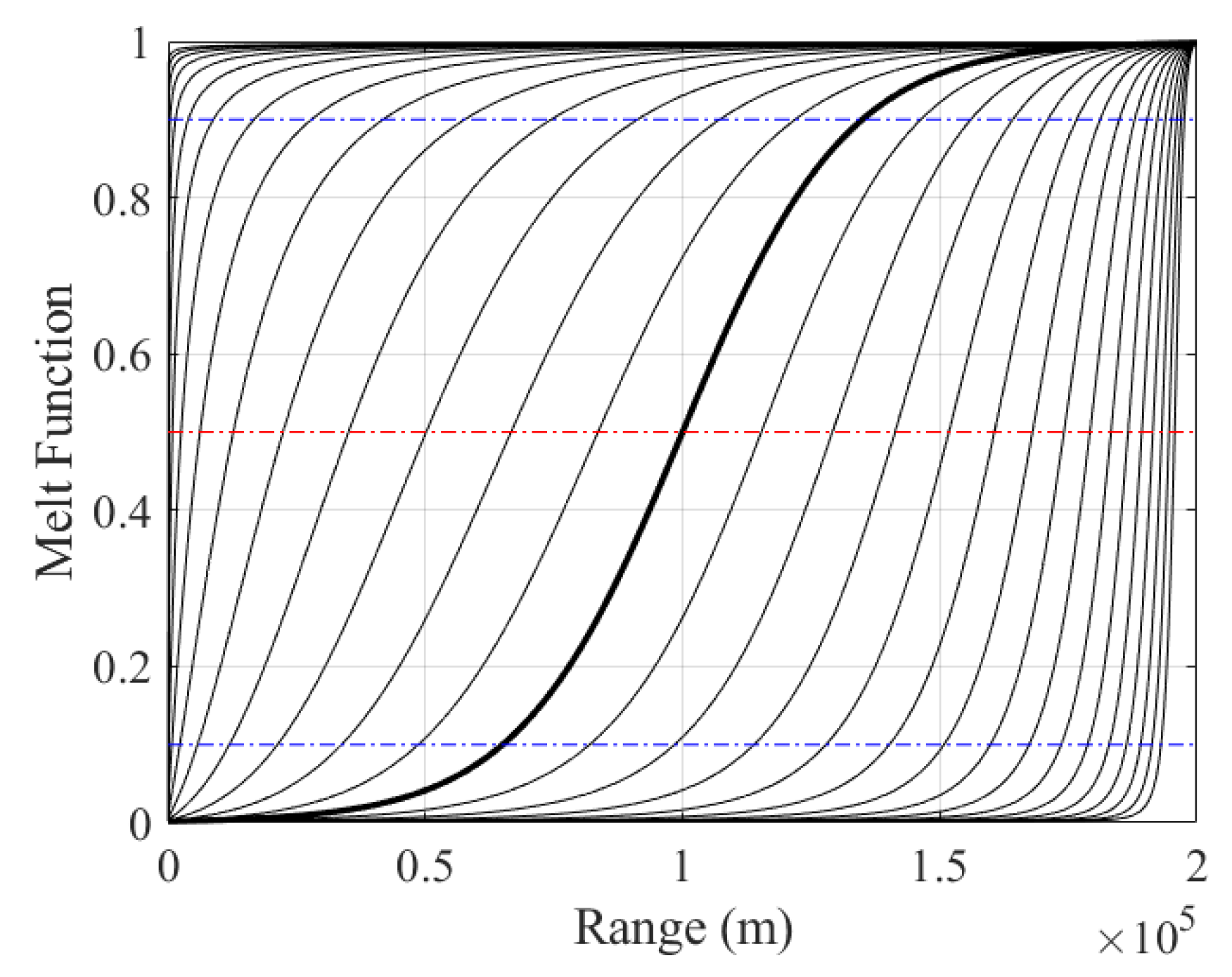
where R is the distance between the two sound speed profiles, and the melt parameter a varies from −1.5 to 1.5. In this paper, since the distance between the north and south of the study area extends across two latitudes, R is defined as 200 km. Figure 3 shows the function curve of melt function m with the melt parameter a in the range of −1.5–1.5. Different melt parameters correspond to different frontal zone positions. Here, we define the initial position of the frontal zone as the position corresponding to when the value of the melt function m is 0.1, and the termination position of the frontal zone as the position corresponding to when the value of the melt function m is 0.9.
According to Equation (3), in order to complete the establishment of the two-dimensional model of the sound speed field of the ocean front, we need to obtain the sound speed profiles of the water masses on both sides of the frontal zone and the melt function related to the distance between the two sound speed profiles. Since the KEF is relatively independent and the water masses on the north and south of the frontal zone are relatively stable, the sound speed profiles at (38° N, 144° E) and (36° N, 144° E) were selected to represent the sound speed profiles of the water masses on the north and south sides of the frontal zone (corresponding to R = 200 km mentioned above). Since different melt parameters a in the melt function correspond to different positions and widths of the frontal zone, the positions and widths of the frontal zone should be obtained first (clustering the surface sound speed of the study area with the fuzzy C-means (FCM) algorithm). Then the values of the corresponding melt parameters can be determined according to Figure 3 to quickly reconstruct the two-dimensional model of the sound speed field of the KEF.
In order to reduce the dependence of ocean front modeling on the data of the whole sea area and the whole sea depth, only the surface sound speed of the study area was clustered with the fuzzy C-means (FCM) algorithm. FCM algorithm was proposed by Bezdek J.C. et al. in the 1980s [30,31]. FCM obtains the membership degree of each sample point to all cluster centers by optimizing the objective function, thereby determining the category of sample points to automatically classify the sample data [32]. In this paper, we use the surface sound speed as data points and cluster the surface sound speed through the FCM algorithm, which has achieved the effect of detecting the frontal zone. There are 26 * 26 = 676 data points in the study area surface, FCM divides 676 sound speed data x i (i = 1, 2,..., 676) into c groups, and identifies the cluster center of each group by minimizing the objective function of the dissimilarity index. The expression of the objective function is as follows:
J ( Q , V ) = k = 1 n i = 1 c ( r i k ) q u k V i 2
where Q is the membership matrix, V is the cluster center, r i k is the membership degree of the k sample point for i category, n is the number of the sample point (in this study, n = 676), c is the number of categories (considering the existence of ocean front, the study area is divided into three water masses, namely, high temperature and salinity water mass located in the south of the frontal zone, low temperature and salinity water mass located in the north of frontal zone south of the frontal zone, and transitional water mass of frontal zone between them, so we set c to 3), q is the weighted index (generally q = 2), and u k V i is the distance between the k sample and the i category. The steps of FCM used in this study are as follows:
(1) Initializing the membership matrix Q with a number between 0 and 1. This step can be completed through translation-standard deviation transformation and translation-range transformation.
The expression of translation-standard deviation transformation is as follows:
x i j = x i j x ¯ j s j ,   ( i ,   j = 1 ,   2 , ,   26 ) ,
x ¯ j = 1 26 i = 1 26 x i j ,   s j = [ 1 26 i = 1 26 ( x i j x ¯ j ) 2 ] 1 2 .
The expression of translation-range transformation is as follows:
x i j = x i j min 1 i 26 { x i j } max 1 i 26 { x i j } min 1 i 26 { x i j }
After transformation, all x i j [ 0 , 1 ] of the sound speed matrix can be obtained, so we complete the initialization of the membership matrix Q .
(2) Calculating the cluster center V ( i ) of the corresponding matrix Q ( i ) .
(3) Updating the membership matrix Q ( i ) and comparing Q ( i ) with Q ( i + 1 ) . If the accuracy δ > 0 (here δ = 10 5 is the default value), max { | r i k ( i + 1 ) r i k ( i ) | } δ , we can get Q ( i + 1 ) and V ( i ) as we want, which is Q = Q ( i + 1 ) , V = V ( i ) . Then, the iteration can be stopped, and the surface sound speed data points are clustered.

2.3. Introduction of Technical Route

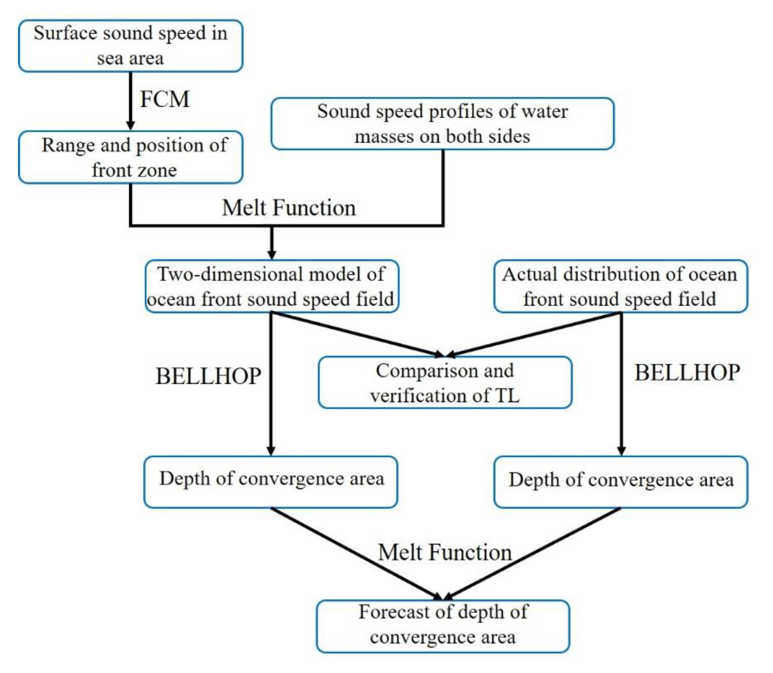
The whole research process is summarized, and the technical route is given as follows (Figure 4). In order to reduce the dependence of ocean front modeling on the data of the whole sea area and the whole sea depth, we only used the sound speed data of sea surface and the SSP of (38° N, 144° E) and (36° N, 144° E) (calculated by Equation (1)). The range and position of the frontal zone can be obtained by using FCM for surface sound speed. Then, the appropriate melt parameter a and melt function m can be selected correspondingly according to the results of FCM, and the sound speed profiles of water masses on both sides can be used as the input of the model to obtain the two-dimensional model of the sound speed field of the ocean front. Compared with the previous research, our research requires less data in this model to quickly obtain the distribution of the sound speed of ocean front. Next, the BELLHOP ray model was used (BELLHOP is an underwater acoustic toolbox for the calculation of the sound field, and we can adjust the parameters through the environment file to get the corresponding sound rays information, multipath information, and so on) to calculate the TL and compare the results of the model with the actual results (calculated by reanalysis data) of the KEF to verify the effectiveness of our model. Finally, we focused on the change of the depth of the acoustic convergence area in the ocean front environment and realized the forecast of the depth of the convergence area by combining the depth of the convergence area in the model and the melt function.

3. Results and Discussion

In this section, we cluster the surface sound speed of the sea with the fuzzy C-means (FCM) algorithm to obtain the position and range of the frontal zone. At the same time, the theoretical model of the ocean front is improved by replacing the temperature profile with the SSP, and the model of the sound speed field of the Kuroshio Extension front (KEF) is established quickly and effectively (Section 3.1). We compare the model with the actual sound speed distribution of the KEF calculated by reanalysis data and verify the validity of the model from the perspective of transmission loss (TL) (Section 3.2). Finally, it is found that the melt function in this model can forecast the depth of the acoustic convergence area in the KEF (Section 3.3).

3.1. Reconstruction Results of Ocean Front Sound Speed Field Model

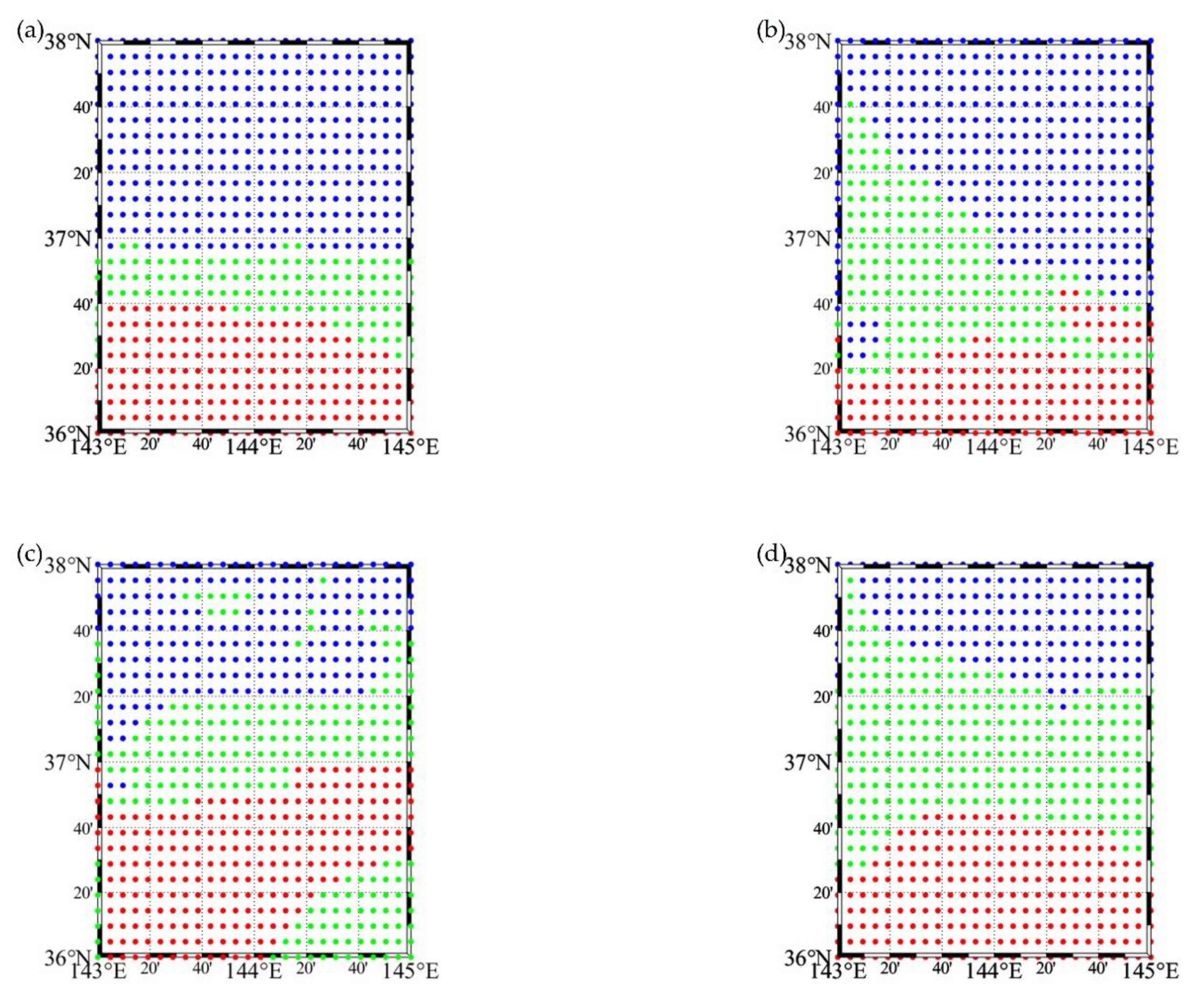
We used FCM to cluster the surface sound speed in the study area, and the results are shown in the figure below (Figure 5). We find that the position, width, and range of the KEF are different at different times.
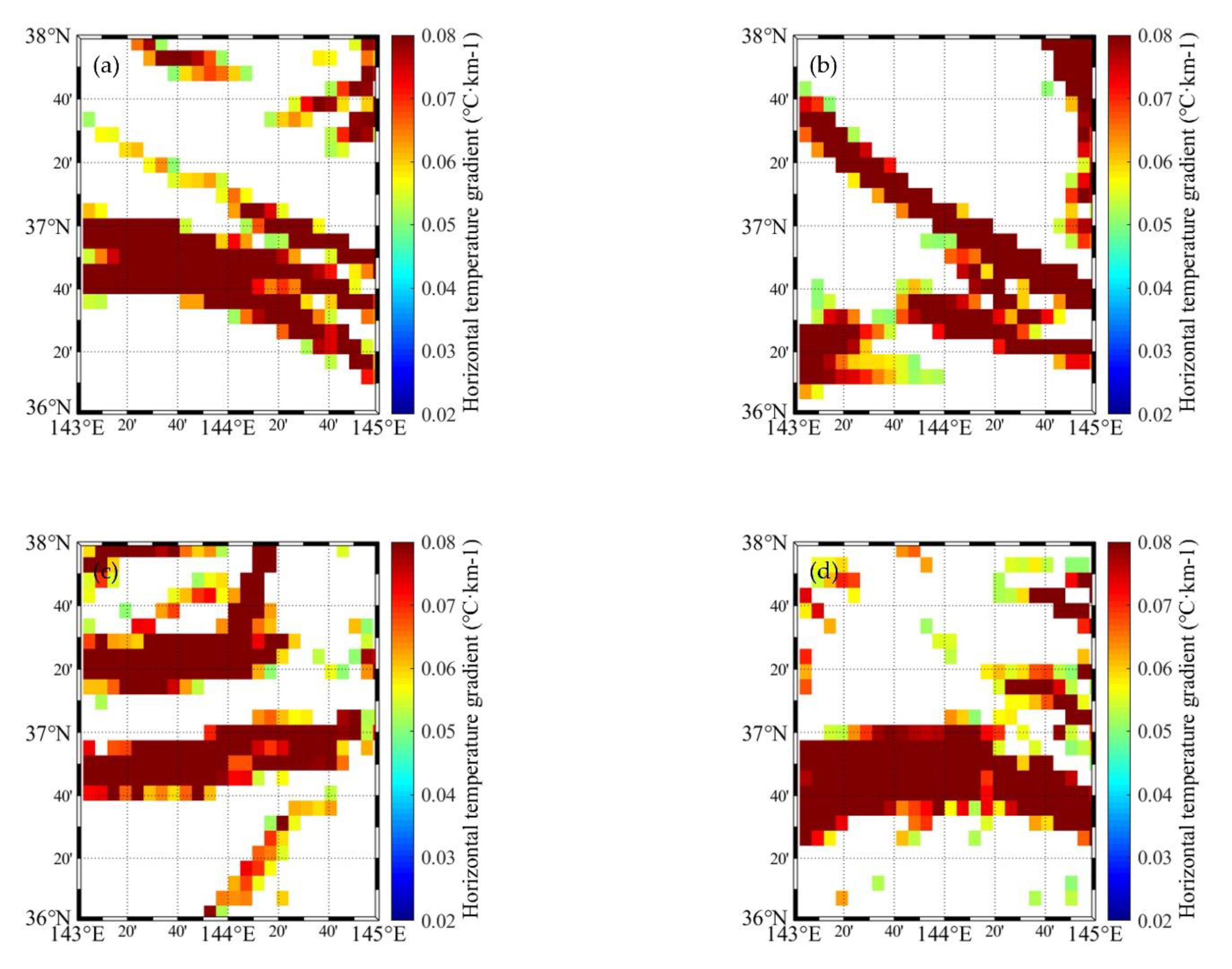
In order to verify the validity of the results of FCM, we calculated the horizontal temperature gradient of the sea surface in the study area to obtain the detection results of the frontal zone under the traditional gradient method (the critical value is 0.05 °C/km) (Figure 6). We found that the detection results of the frontal zone were similar to those of the FCM, especially in winter (Figure 6a,b). Compared with those of the gradient method, the detection results of FCM led to a more continuous frontal zone in the range, which is helpful for us to obtain the starting and ending positions of the frontal zone on the relevant sections and realize effective modeling. However, the continuity of the judgment results of the temperature gradient method is very poor, and this discontinuity may become worse due to different judgment standards.
The 144 °E was selected as the characteristic section (the direction is 38° N–36° N). According to the results of FCM (Figure 5) and the function curve of melt function m with melt parameter a (Figure 3), we identified the position and range of the frontal zone of KEF at different times as well as the selection of the corresponding melt parameters (Table 1). The melt parameters a of the model of the sound speed field of the ocean front in four periods were determined as 0.2, 0.3, 0, and −0.1, respectively.
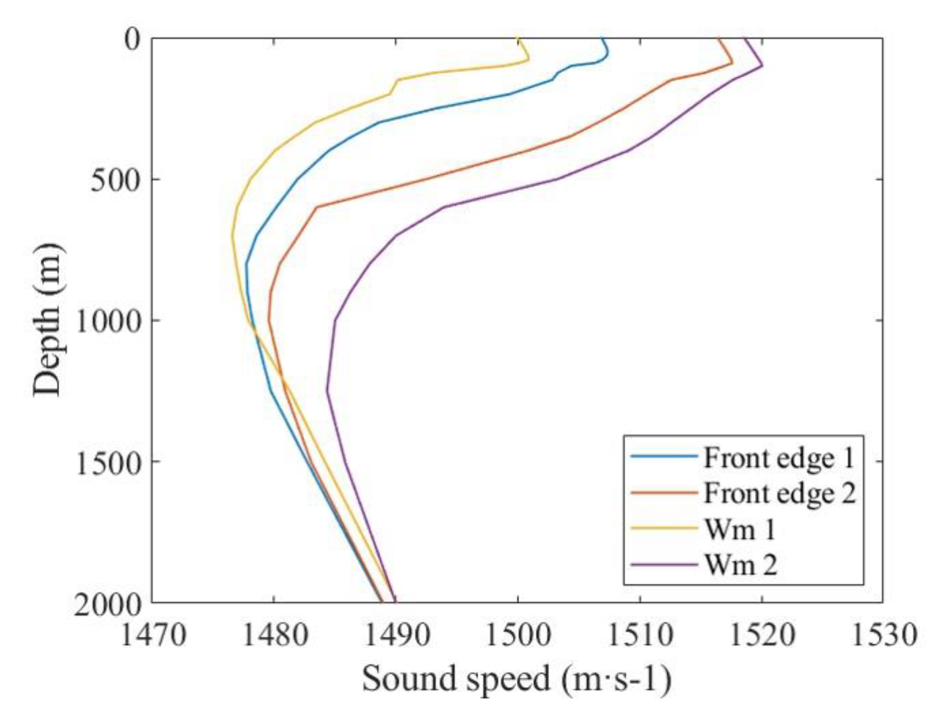
Taking the experiment on 1 January as an example, we obtained the sound speed profiles of water masses on both sides of the frontal zone ((38° N, 144° E) and (36° N, 144° E)) and the sound speed profiles on the edge of the frontal zone (Figure 7). We found obvious differences between the sound speed profiles of water masses on both sides of the frontal zone. The depth of the SOFAR axis (the depth of the minimum sound speed) of the SSP on the north side was deeper, and the surface sound speed difference between the water masses on the south side and the north side was more than 18 m/s. Between the front edge, 1 and 2 are the sound speed profiles in the frontal zone.
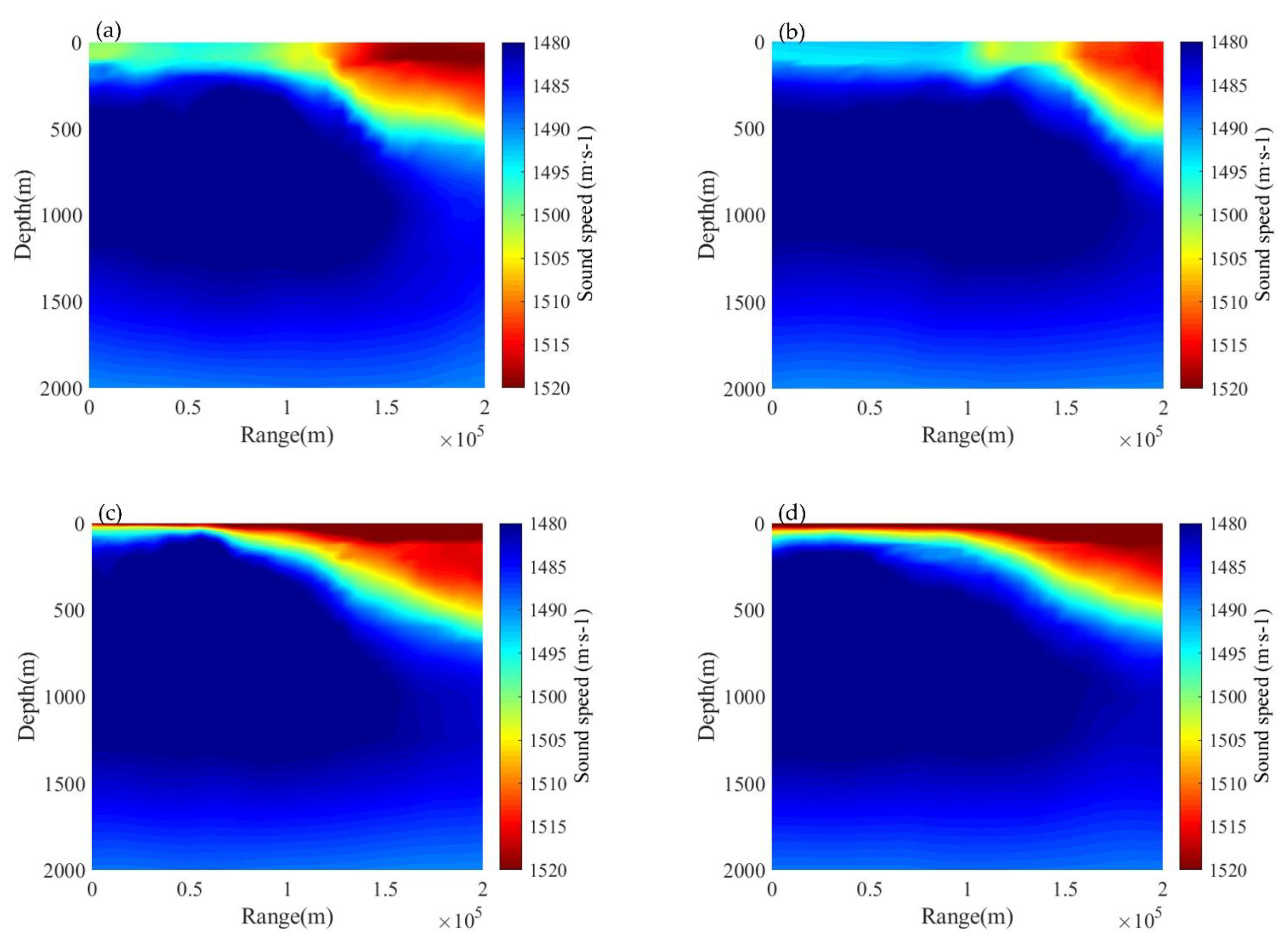
According to the melt parameters determined at different times and the sound speed profiles at points (38° N, 144° E) and (36° N, 144° E), the model of the sound speed field of the KEF was established quickly (Figure 8). We found that the distribution of sound speed obtained by the overall model was similar to that of the actual KEF (Figure 2) in terms of the location of the front and the depth of the influence (especially in winter). However, since there are other mesoscale or submesoscale processes such as internal waves in the actual sea water [33,34], and only two typical water mass sound speed profiles and the location information of frontal zone was extracted as input in our model, the results of the model are still different from the actual distribution of the sound speed of the ocean front in detail. Next, the effectiveness of the model was analyzed through the results of the TL calculation.

3.2. Comparison Results of TL Calculations

The BELLHOP ray model was used to calculate the TL of our model and the actual KEF environment. Compared with the normal mode model or parabolic equation model, the ray model can clearly describe the change of sound energy in the process of propagation, which is more suitable for the ocean front environment in this paper. The parameter settings in the sound field calculation process are as follows: the sound source frequencies were set to 50 Hz and 400 Hz, the glancing angle was −20°–20°, the sound source depth (SD) was 100 m, 300 m, and 500 m, and the receiving depth remained the same as the SD. The seabed sound speed is 1600 m/s, the density was 1.8 g/cm3, and the sound absorption coefficient of the seabed was 0.8 dB/λ.
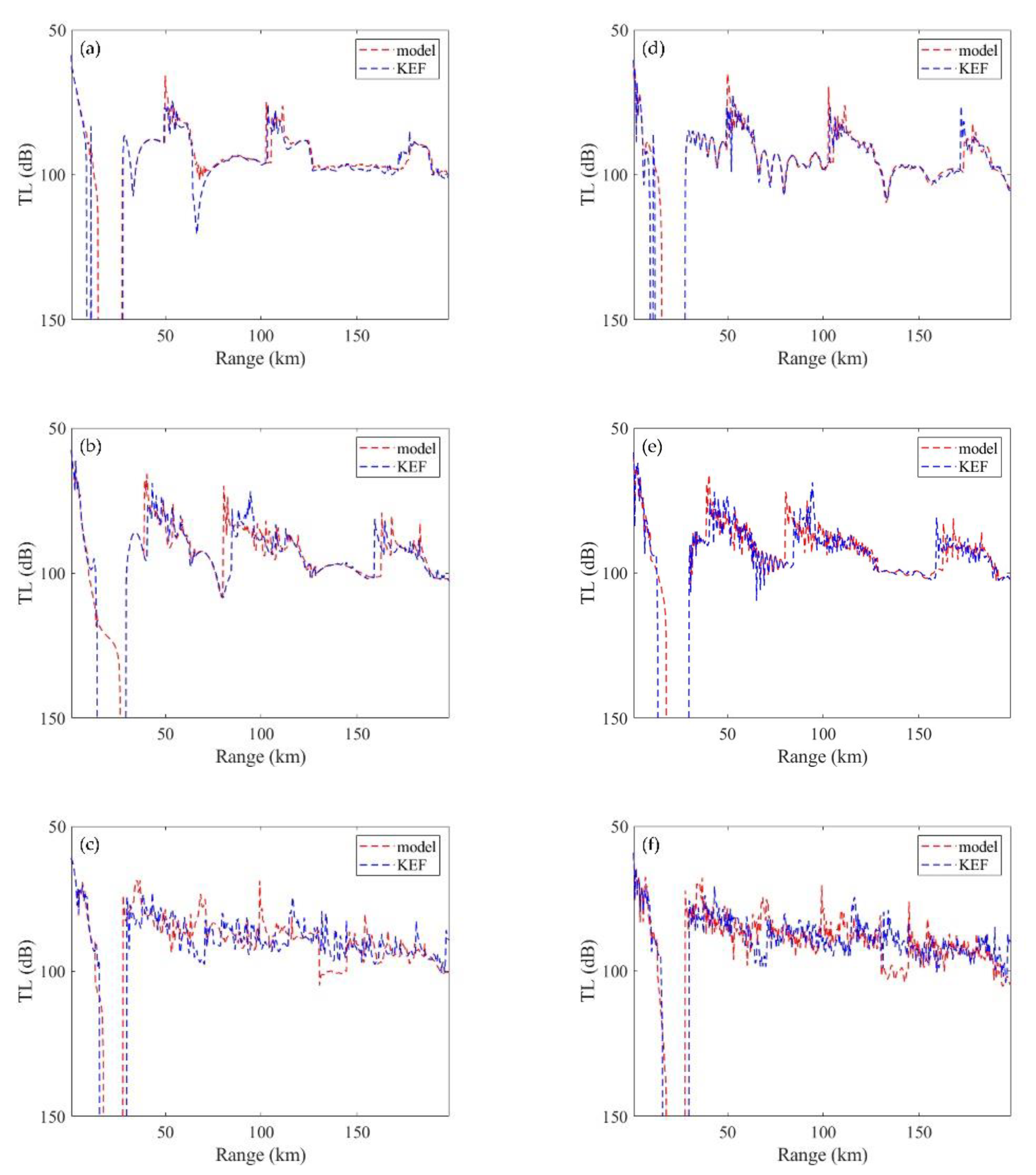
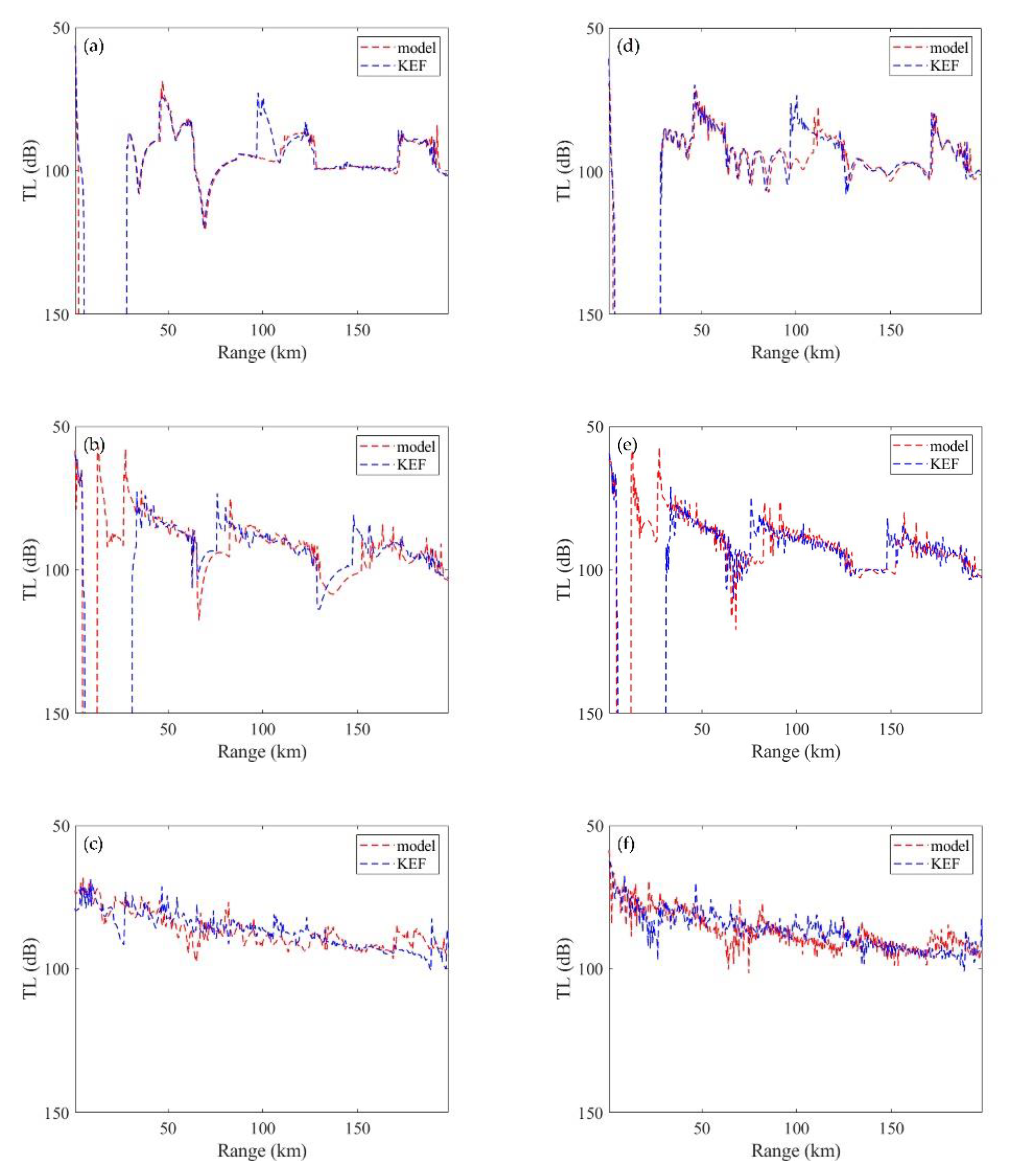
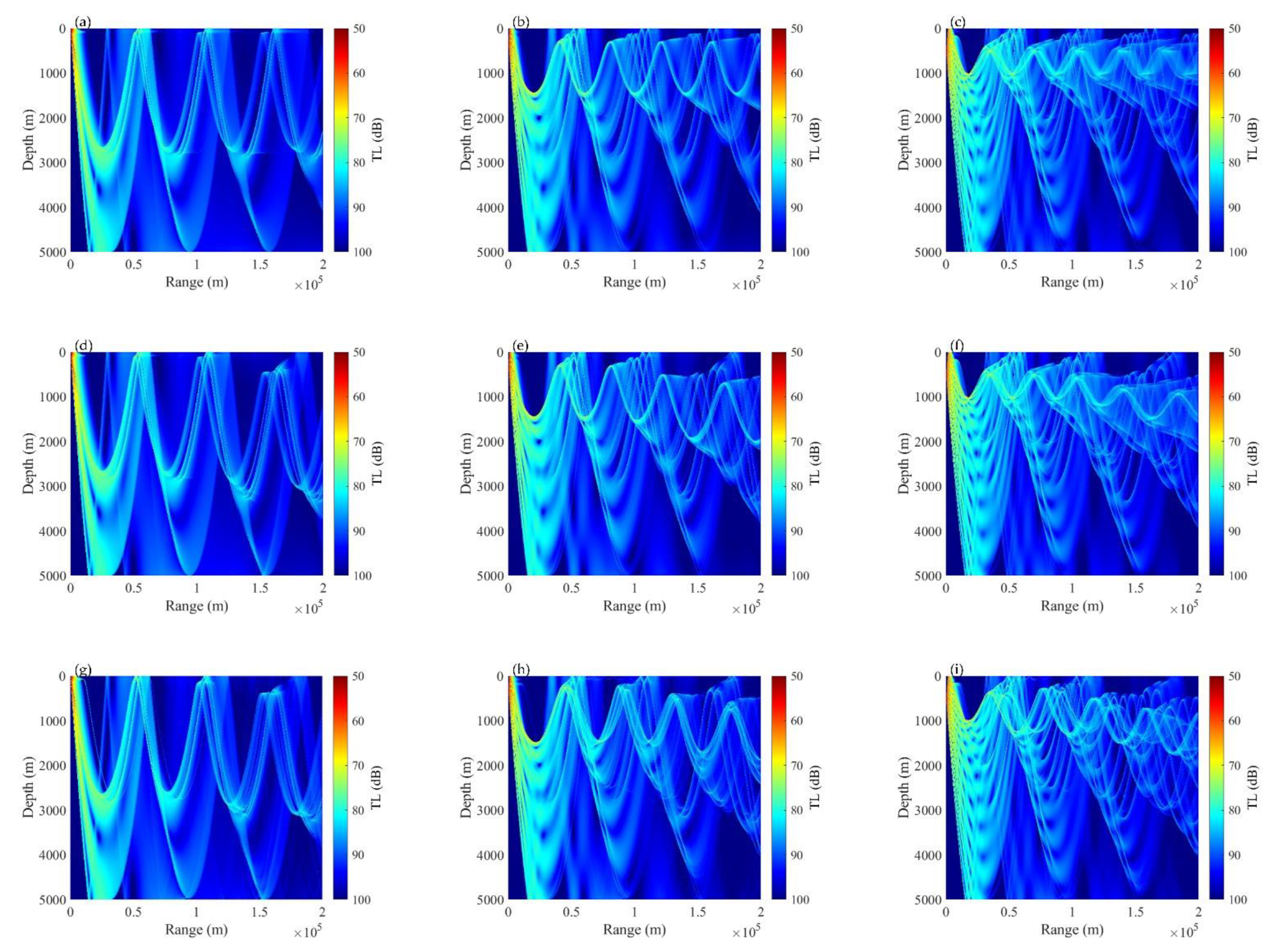
We respectively calculated the TL under the model environment and the actual ocean front environment at different times (Figure 9, Figure 10, Figure 11 and Figure 12). We found that when the SD was 100 m, the difference between the TL calculated by the model and the TL calculated by the actual ocean front was very small at low and high frequencies. The result of the model at 100 m can well replace the actual TL; at 300 m, only on February 1st (Figure 10b,e), the calculation results of low frequency and high frequency showed a small difference after passing the frontal zone, but in terms of the overall distribution trend, the results of the model were similar to the calculation results under the actual ocean front environment; at a deeper emission depth (SD = 500 m), since the SD is close to the SOFAR axis, there was no obvious convergence area or shadow area phenomenon in the distribution of TL, but in terms of the overall trend, the results of the model and the actual results also showed many similarities.
In order to quantify the simulation results of the model, we smoothed the above results through the five-point smoothing method and calculated the root means square error (RMSE) and the percentage with the difference exceeding 10 dB compared with the actual TL (Table 2). It was found that before smoothing, the RMSE of the model was mostly controlled below 6 dB compared with the actual results. Compared with that in previous studies, the effect was further improved. Before smoothing, the percentage with the difference exceeding 10 dB was maintained near 10%, which indicated that the results of our model were less fluctuating than the actual results. In terms of RMSE, all smoothed data were reduced to less than 6 dB, and the percentage with the difference exceeding 10 dB was also further reduced. Except for individual data near 10%, most of the data had been reduced to less than 8%, which verified the effectiveness of the model. As to TL, the calculation results of the model were in good agreement with the actual situation.
We calculated the RMSE under different sound source frequencies (Table 3) and different sound source depths (Table 4) to compare the differences between winter (the dates were 0101 and 0201) and summer (the dates were 0701 and 0801). We found that when frequencies were different, the RMSE of TL was close to the same in different seasons, and the seasonal difference of the RMSE caused by the change of frequency was not obvious. When sound source depths were different, the RMSE of TL was different between winter and summer. Specifically, when SD = 100 m, the RMSE in winter was less than that in summer (the difference of unsmoothed results was about 1 dB); When SD = 300 m, the unsmoothed results of the two seasons were equivalent; when SD = 500 m, the RMSE in winter was less than that in summer (the difference of unsmoothed results was still about 1 dB). Analyzing the reasons for the difference of the RMSE of TL under different sound source depths in the two seasons, we believed that in terms of the frontal zone position and influence depth, the sound speed distribution obtained by the model in winter was more similar to the actual KEF distribution than that in summer (Figure 8). Therefore, when the sound source and reception depth were shallow, the RMSE of TL obtained in winter was smaller; at deeper depths, the phenomenon of convergence area is no longer obvious compared with that of shallow sound source depth (Figure 9c,f and Figure 12c,f), the RMSE may be greater in winter than in summer (this level was only less than 1 dB, which was acceptable, but we can not deny that the effectiveness of the model in winter was better).

3.3. Effectiveness of Forecasting the Changes of Depth in Convergence Areas

The convergence area is the area where the sound energy is concentrated near the sea surface during the sound propagation process [35]. The study of the convergence area is of practical significance for underwater acoustic detection [36,37]. Due to the existence of the ocean front, the depth change of the convergence area has become a concern. Taking the experiment on January 1st as an example, we set the sound source frequency to 50 Hz, and calculated the whole sea depth variation of the TL in the distance-independent environment (the environment without ocean fronts), model environment, and the actual ocean front environment at the SD of 100 m, 300 m, and 500 m (Figure 13). It was found that due to the existence of the ocean front, there was a significant downward shift in the distribution of TL after its passing through the frontal zone in the convergence area, which was a very obvious phenomenon is in both the model and the actual ocean front environments. The change in the depth of the convergence area is related to not only the SD but also the location of the frontal zone and the range of its influence. Since the effectiveness of the model from the perspective of TL is verified in the previous section, in this section the effectiveness of melt function in the rapid forecast of the convergence area depth in the ocean front environment is verified by combining the melt function with the depth of the convergence area calculated by the model and the actual ocean front.
The law of refraction followed by ray acoustics is Snell’s law:
cos α 0 c 0 = cos α i c i = c o n s t
where α 0 is the angle between the incident direction and the horizontal direction of the sound rays, called grazing angle, c 0 is the sound speed on the medium surface of the incident layer, α i and c i is the grazing angle and sound speed of the sound rays on the surface of the outgoing layer respectively. According to Snell’s law, when the sound speed changes with depth, the sound rays always bend to the place where the sound speed is lower. The convergence area is a manifestation of the concentrated area of sound ray turning, so the depth of the convergence area is not only related to the SD but also has a corresponding relationship with the distribution of sound speed.
Since only the sound speed profiles of the water masses on both sides of the frontal zone were used in our model as input values, we only obtained the data of these two sound speed profiles. Taking the experiment on January 1st as an example, the SOFAR axis depth of these two sound speed profiles was 700 m and 1250 m, respectively (Figure 7). When the SD is fixed, according to Snell’s law, the depth of the convergence area formed by the sound rays emitted at a small glancing angle near the sound source should be basically the same as the SD (or slightly shallower than the SD) under a distance-independent environment. As shown in Figure 13, when the SD is 100 m, 300 m, and 500 m, the depth of the convergence area always stays near 0 m (Figure 13a), 200 m (Figure 13b), and 400 m (Figure 13c) under a distance-independent environment. In our model and actual ocean front environment, when the SD is located at 100 m, 300 m, and 500 m, the depth of the convergence area near the sound source is 0 m (Figure 13d,g), 200 m (Figure 13e,h), and 400 m (Figure 13f,i), respectively since the ocean environment not far away from the sound source is also a distance-independent environment. Based on the above analysis, we obtained a forecast curve of the depth change of the convergence area during the transmission process in the ocean front environment:
D ( z ) = D 1 ( z ) + m ( r ; a ) [ D 2 ( z ) D 1 ( z ) ]
where D 1 ( z ) is the depth of the convergence area near the sound source, D 2 ( z ) is the depth of the convergence area at the farthest distance (200 km). m ( r ; a ) is the melt function, and the expression is consistent with Equation (4). In the ocean front environment, it is believed that the depth change of the convergence area is related to the change of the sound speed. Therefore, the depth of the SOFAR axis was extracted as the feedback depth and to estimate D 2 ( z ) :
D 2 ( z ) D 1 ( z ) = S O F A R 2 ( z ) S O F A R 1 ( z )
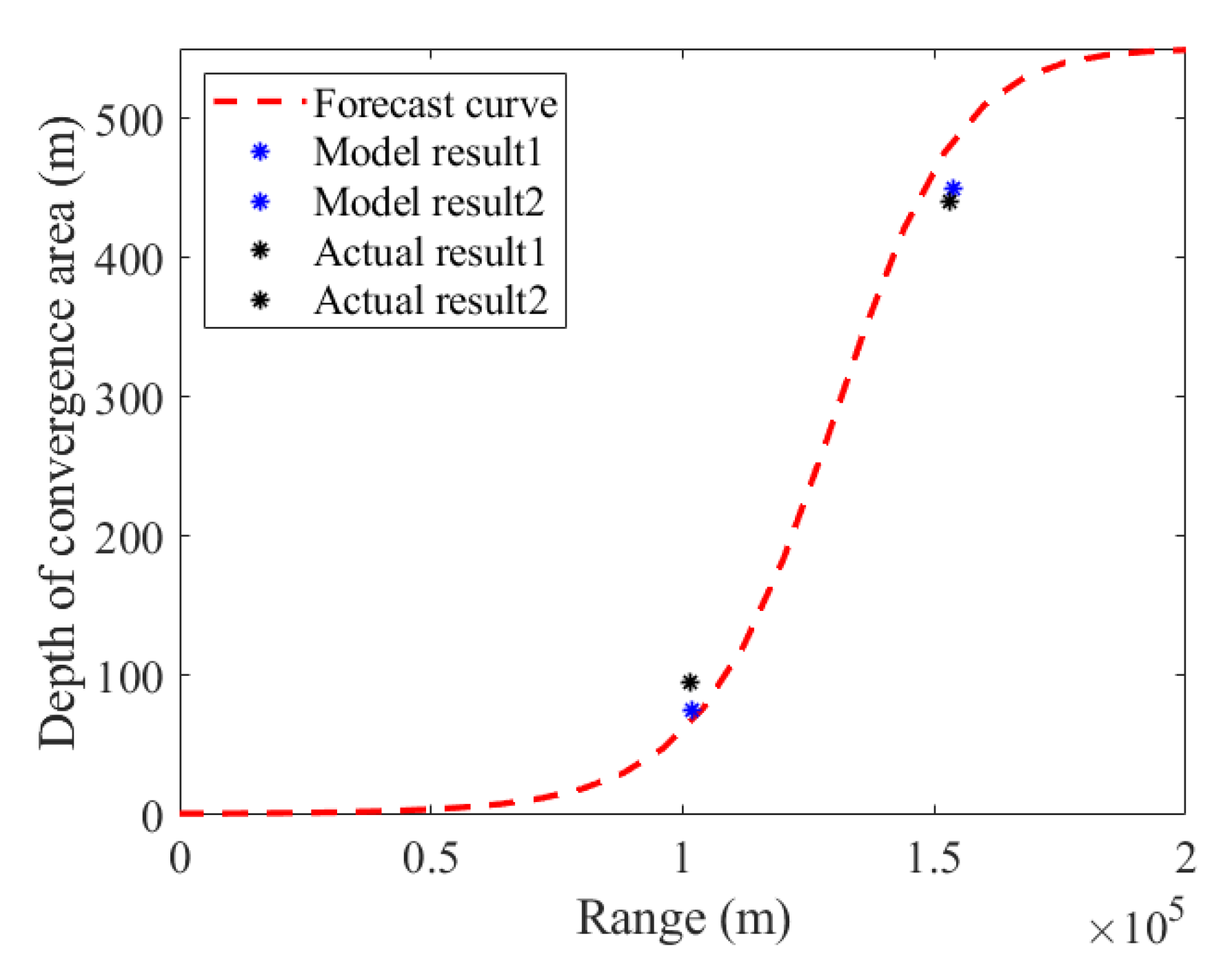
where S O F A R 1 ( z ) and S O F A R 2 ( z ) are the depths of the SOFAR axis of two sound speed profiles. Take the experiment on January 1st as an example, the S O F A R 1 ( z ) and S O F A R 2 ( z ) are known to be 700 m and 1250 m. When the SD = 100 m, the depth of the convergence area near the sound source was about 0 m ( D 1 ( z ) =0 m), so D 2 ( z ) should be 550 m. We completed the forecast of the depth of the convergence area at the SD of 100 m on 1 January and compared this result with the model calculated one (we selected two convergence areas passing through the frontal zone) and the actual results of the ocean front (corresponding to the two convergence areas of the model), to obtain the following results (Figure 14). We found that the depth distribution of the convergence area in the model and the actual condition were in good agreement with the forecasted curve with only a little difference, which proves that the melt function was applied to effectively achieve the depth forecast of the convergence area in the ocean front environment.
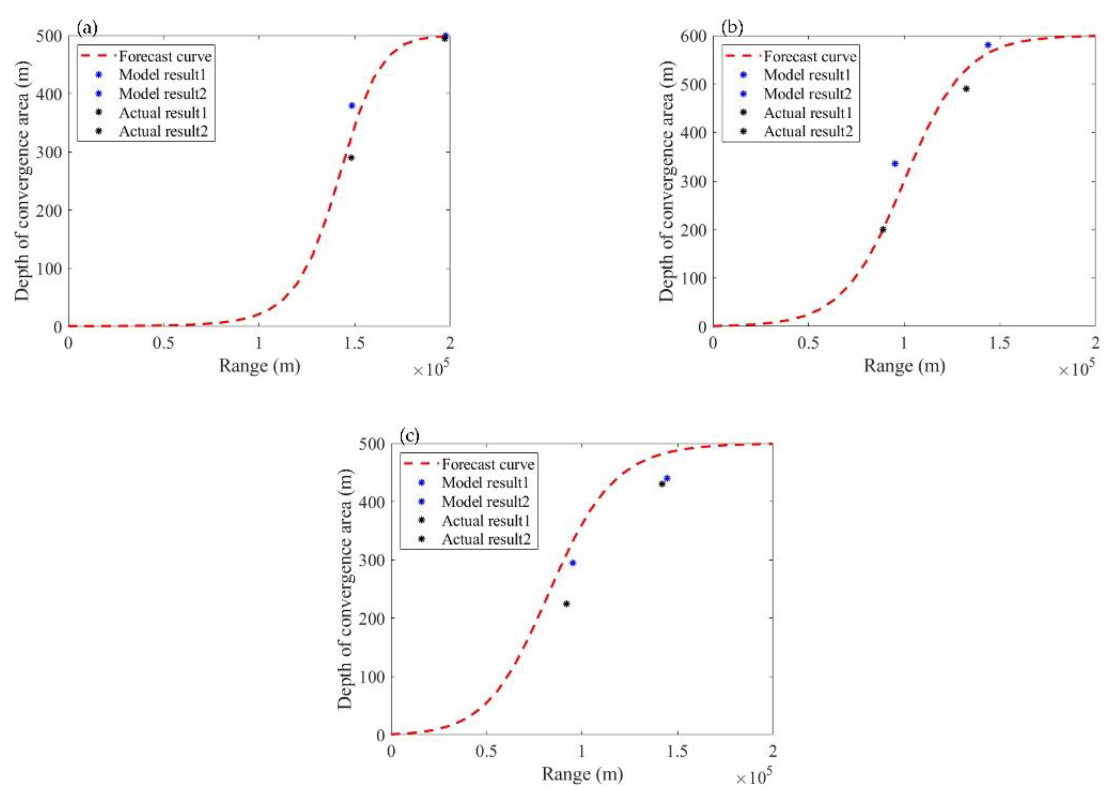
By respectively analyzing the results of the depth of the convergence area during the four periods (Figure 14 and Figure 15), it was concluded that since the two sound speed profiles were different in different periods when the SD was fixed, the depth of the convergence area is related to that of the SOFAR axis, the difference between them, as well as the SD. The forecasting results using the melt function based on the melt parameter a (which is related to the width and location of the frontal zone) were in good agreement with the model and the actual results, which proves the effectiveness of this method.
By calculating the forecasting results of other sound source depths together (Table 5), it was found that when the SD was shallow, the forecasting results were in good agreement with the actual results, but the degree of agreement was relatively poor at a deeper launch depth (SD = 500 m) because SD’s closeness to the SOFAR axis makes most of the sound energy converge near the SOFAR axis and propagates forward. It is impossible to form an obvious convergence area, which can not be detected during some periods. After calculation, the RMSE between the forecasting results and model calculation results in the first detection convergence area was 74.8 m, and the second detection convergence area was 45.0 m; The RMSE between the forecasting results and the actual calculation results in the first detection convergence area was 82.3 m, and the second detection convergence area was 43.3 m. It shows that the RMSE of the second detection convergence area was smaller and the effectiveness of forecasting was better.

4. Summary and Conclusions

In this paper, we first used the fuzzy C-means clustering method to perform fuzzy clustering on the surface sound speed of the Kuroshio extension study area and obtained the range and location of the frontal zone. The result of cluster analysis can be consistent with the result of surface temperature gradient judgment. Next, according to the position and range of the frontal zone at different times, we selected the corresponding melt parameters to construct a two-dimensional parametric model of ocean fronts based on the sound speed profile. The results showed that it had a good similarity with the actual two-dimensional sound speed distribution of the ocean front. In order to verify the effectiveness of the ocean front model in acoustic forecasting, we selected a characteristic section and used the BELLHOP ray model to obtain the comparison between the model and the actual transmission loss by setting different sound source depths and emission frequencies. It was found that the root means square error between the calculated results of the model and the actual results was mostly controlled below 6 dB. As far as the percentage with the difference exceeding 10 dB is concerned, this level was basically maintained at around 10%. In terms of the transmission loss, the calculation results of the model were in good agreement with the actual situation. Finally, we proposed a simple combination of the melt function and the depth of the convergence area to verify the effectiveness of applying the melt function to the rapid forecasting of the depth of the convergence area in the ocean front environment. After calculation, the root mean square error between the forecasting result and the actual calculation result in the first detection convergence area was 82.3 m, and the second detection convergence area was 43.3 m, the forecasting effect was better. It is hoped that this research may be to some degree of referential significance to acoustic detection in the ocean front environment.
As one of the most common mesoscale phenomena in the ocean, the impact of ocean fronts on underwater acoustic detection has become a hot spot for hydroacoustics. Because experimental data with high spatial resolution in the ocean front area can not be quickly and effectively obtained by oceanographic surveys, it is feasible to use theoretical models combined with typical data to reconstruct ocean fronts and analyze their impact on acoustic detection. Therefore, according to our method, future oceanographic surveys only require surface sound speed data (of course, this part of the data can also be obtained through the satellite remote sensing data of high spatial resolution) and sound speed profiles representing the typical properties of water masses (this part of the data can be obtained through the actual ocean surveys). Then we can construct the two-dimensional sound speed field distribution model in the ocean front environment. This method was proven effective in our research. This method can effectively predict the depth of the convergence area and can also provide us with relevant help in the acoustic detection of the relevant sea areas in the ocean front. For example, the decline of the depth of the convergence area is unfavorable to the acoustic detection under certain conditions, and this method can capture this disadvantage in advance.
It should be pointed out that although we have proved the applicability of this method to KEF in this paper, we have not proved whether this method is applicable in other ocean front environments. This is also one of the key points of future research. In addition, we also need to further study the interference of other ocean phenomena such as internal waves on the two-dimensional sound speed field modeling of ocean front.

Author Contributions

Conceptualization, W.C. (Wei Chen), Y.L. and L.M.; methodology, Y.L. and W.C. (Wen Chen); software, Y.C.; validation, Y.L.; formal analysis, Y.C. and Z.M.; investigation, W.C. (Wen Chen) and Y.L.; writing—original draft preparation, Y.L. and W.C. (Wei Chen); writing—review and editing, W.C. (Wei Chen) and L.M.; funding acquisition, Y.C. All authors have read and agreed to the published version of the manuscript.

Funding

This research was funded by the National Natural Science Foundation of China under contract No. 61901488.

Institutional Review Board Statement

Not applicable.

Informed Consent Statement

Not applicable.

Data Availability Statement

Not applicable.

Conflicts of Interest

The authors declare no conflict of interest.

References

  1. Belkin, I.M.; Cornillon, P.C.; Sherman, K. Fronts in large marine ecosystems. Prog. Oceanogr. 2009, 81, 223–236. [Google Scholar] [CrossRef]
  2. Bost, C.A.; Cotté, C.; Bailleul, F.; Cherel, Y.; Charrassin, J.B.; Guinet, C. The importance of oceanographic fronts to marine birds and mammals of the southern oceans. J Mar Syst. 2009, 78, 363–376. [Google Scholar] [CrossRef]
  3. Peter, C.; Wang, G. Seasonal variability of thermohaline front in the central South China Sea. J. Oceanogr. 2003, 59, 65–78. [Google Scholar] [CrossRef]
  4. Avijit, G.; Allan, R. Feature-oriented regional modeling of oceanic fronts. Dyn. Atmos. Ocean. 2002, 36, 201–232. [Google Scholar]
  5. Moore, J.K.; Abbott, M.R.; Richman, J.G. Variability in the location of the Antarctic Polar Front (90°–20°W) from satellite sea surface temperature data. J. Geophys. Res. Ocean. 1997, 102, 27825–27833. [Google Scholar] [CrossRef] [Green Version]
  6. Chen, B.; Liang, M.A.; Zhang, C.; Bing, L.I.; Liu, H. Ocean front analysis in subdivided sea areas by using satellite remote sea surface temperature data. Ocean. Eng. 2018, 36, 108–118. [Google Scholar]
  7. Shapiro, G.; Chen, F.; Thain, R. The effect of ocean fronts on acoustic wave propagation in the Celtic sea. J Mar. Syst. 2014, 139, 217–226. [Google Scholar] [CrossRef]
  8. Mooers, C.N.K. Oceanic fronts and their effects on underwater acoustics. J. Acoust. Soc. Am. 1978, 63, S87. [Google Scholar] [CrossRef]
  9. Rousseau, T.H. Acoustic propagation through a model of shallow fronts in the deep ocean. J. Acoust. Soc. Am. 1982, 72, 924–936. [Google Scholar] [CrossRef]
  10. Ramp, S.R.; Chiu, C.S.; Bahr, F.L.; Qi, Y.; Dahl, P.H.; Miller, J.; Lynch, J.F.; Zhang, R.; Zhou, J. The shelf-edge frontal structure in the central East China Sea and its impact on low-frequency acoustic propagation. IEEE J. Ocean. Eng. 2005, 29, 1011–1031. [Google Scholar] [CrossRef]
  11. Rajkumar, K.V.; Yesubabu, A.; Subrahmanyam, K. Fuzzy clustering and Fuzzy C-Means partition cluster analysis and validation studies on a subset of citescore dataset. Int. J. Electr. Comput. Eng. 2019, 9, 2760–2770. [Google Scholar] [CrossRef]
  12. Mandelberg, M.D.; Frizzell-Makowski, L.J. Acoustic provincing of ocean basins. Ocean. 2000 MTS IEEE Conf. Exhib. 2000, 105–108. [Google Scholar] [CrossRef]
  13. Abiva, J.; Fabbri, T.; Raúl, V. Automatic classification of sound speed profiles using PCA and Self-Organizing Map techniques. Ocean. 2019- Marseille IEEE 2019, 1–10. [Google Scholar] [CrossRef]
  14. Dubberley, J.; Zingerelli, R. Fuzzy clustering of oceanographic sound speed profiles for acoustic characterization. J. Acoust. Soc. Am. 2008, 123, 3625. [Google Scholar] [CrossRef]
  15. Chen, C.; Yang, K.; Duan, R.; Ma, Y. Acoustic propagation analysis with a sound speed feature model in the front area of kuroshio extension. Appl. Ocean. Res. 2017, 68, 1–10. [Google Scholar] [CrossRef]
  16. Gangopadhyay, A.; Robinson, A.R.; Haley, P.J.; Leslie, W.G.; Yu, Z. Feature-oriented regional modeling and simulations in the Gulf of Maine and Georges Bank. Cont. Shelf Res. 2003, 23, 317–353. [Google Scholar] [CrossRef]
  17. Carriere, O.; Hermand, J.P. Feature-oriented acoustic tomography for coastal ocean observatories. IEEE J. Ocean. Eng. 2013, 38, 534–546. [Google Scholar] [CrossRef]
  18. Lin, Y.T.; Lynch, J.F. Analytical study of the horizontal ducting of sound by an oceanic front over a slope. J. Acoust. Soc. Am. 2012, 131, EL1. [Google Scholar] [CrossRef] [PubMed] [Green Version]
  19. Ramp, S.R.; Schlitz, R.J.; Wright, W.R. The deep flow through the northeast channel, Gulf of Marine. J. Phys. Oceanogr. 1985, 15, 1790–1808. [Google Scholar] [CrossRef] [Green Version]
  20. Small, J.; Shackleford, L.; Pavey, G. Ocean feature models-their use and effectiveness in ocean acoustic forecasting. Ann. Geophys. 1997, 15, 101–112. [Google Scholar] [CrossRef]
  21. Kwon, Y.O.; Alexander, M.A.; Bond, N.A.; Frankignoul, C.; Lu, A.T. Role of the gulf stream and kuroshio–oyashio systems in large-scale atmosphere–ocean interaction: A review. J. Clim. 2010, 23, 3249–3281. [Google Scholar] [CrossRef]
  22. Xue, H.J.; Chai, F.; Pettigrew, N.; Xu, D.Y.; Shi, M.C.; Xu, J.P. Kuroshio intrusion and the circulation in the south china sea. J. Geophys. Res. Ocean. 2004, 109, 1–14. [Google Scholar] [CrossRef] [Green Version]
  23. Yasuda, I.; Yoon, J.H.; Suginohara, N. Dynamics of the Kuroshio large meander. J. Oceanogr. Soc. Jpn. 1985, 41, 259–273. [Google Scholar] [CrossRef]
  24. Li, Y.; Kang, J.C.; Liu, C. Spatial change of salinity at Kuroshio in East China Sea with seasons. Appl. Mech. Mater. 2011, 71–78, 56–60. [Google Scholar] [CrossRef]
  25. Imawaki, S.; Uchida, H.; Ichikawa, H.; Fukasawa, M.; Umatani, S.I. Satellite altimeter monitoring the Kuroshio transport south of Japan. Geophys. Res. Lett. 2001, 28, 17–20. [Google Scholar] [CrossRef]
  26. Nonaka, M.; Xie, S.P. Covariations of sea surface temperature and wind over the Kuroshio and its extension: Evidence for ocean-to-atmosphere feedback. J. Clim. 2003, 16, 1404–1413. [Google Scholar] [CrossRef]
  27. Chassignet, E.P.; Hulburt, H.E.; Smedstad, O.M.; Halliwell, G.R.; Hogan, P.J. The HYCOM (HYbrid Coordinate Ocean Model) data assimilative system. J. Mar. Syst. 2007, 65, 60–83. [Google Scholar] [CrossRef]
  28. Chassignet, E.P.; Smith, L.T.; Halliwell, G.R.; Bleck, R. North Atlantic simulations with the Hybrid Coordinate Ocean Model (HYCOM): Impact of the vertical coordinate choice, reference pressure, and thermobaricity. J. Phys. Oceanogr. 2003, 33, 2504–2526. [Google Scholar] [CrossRef] [Green Version]
  29. Medwin, H. Speed of sound in water: A simple equation for realistic parameters. J. Acoust. Soc. Am. 1975, 58, 1318–1319. [Google Scholar] [CrossRef]
  30. Bezdek, J.C.; Ehrlich, R.; Full, W. FCM: The fuzzy c -means clustering algorithm. Comput. Geosci. 1984, 10, 191–203. [Google Scholar] [CrossRef]
  31. Bezdek, J.C. A Convergence Theorem for the Fuzzy ISODATA Clustering Algorithms. IEEE Trans. Pattern Anal. Mach. Intell. 1980, 2, 1–8. [Google Scholar] [CrossRef]
  32. Arkajyoti, S.; Swagatam, D. Axiomatic generalization of the membership degree based weighting function for fuzzy C means clustering: Theoretical development and convergence analysis. Inf. Sci. 2017, 408, 129–145. [Google Scholar] [CrossRef]
  33. Andreeva, T.A.; Durgin, W.W.; Wojcik, S.E. Influence of internal wave fluctuations on acoustic underwater propagation. J. Acoust. Soc. Am. 2005, 117, 2548. [Google Scholar] [CrossRef]
  34. Ju, L.; Wang, H.; Sun, J. Effect of tidal internal wave fields on shallow water acoustic propagation. AIP Conf. Proc. 2010, 191, 1272. [Google Scholar] [CrossRef]
  35. Hale, F.E. Long-range sound propagation in the deep ocean. J. Acoust. Soc. Am. 1959, 31, 1572. [Google Scholar] [CrossRef] [Green Version]
  36. Mellberg, L.E.; Johannessen, O.M.; Connors, D.N.; Botseas, G.; Browning, D. Modeled acoustic propagation through an ice edge eddy in the east greenland sea marginal ice zone. J. Geophys. Res. Oceans. 1987, 92, C7. [Google Scholar] [CrossRef]
  37. Lynch, J.F.; Newhall, A.E.; Sperry, B.; Gawarkiewicz, G.; Fredricks, A.; Tyack, P.; Chiu, C.S.; Abbot, P. Spatial and temporal variations in acoustic propagation characteristics at the New England shelfbreak front. IEEE J. Ocean. Eng. 2003, 28, 129–150. [Google Scholar] [CrossRef]
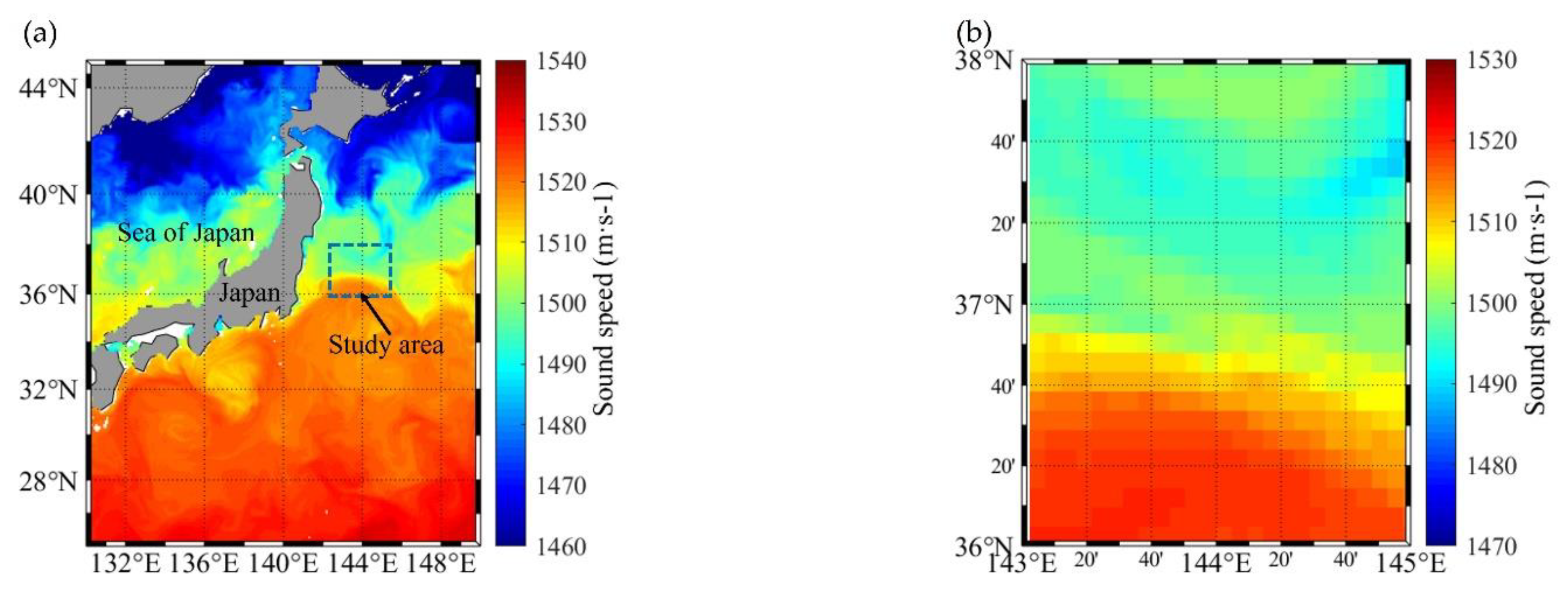
Figure 1. (a) The surface sound speed of parts of the Northwest Pacific and the location of the study area; (b) The sea surface sound speed distribution of the study area on 1 January 2019. The KEF divides the sea area into three water masses, namely, the low temperature and low salinity water mass in the north of the frontal zone, the high temperature and high salinity water mass in the south of the frontal zone, and the frontal transitional water mass between them.
Applsci 11 08461 g001
Figure 2. Sound speed distribution of the 144° E section in different periods in the ocean front environment (the depth of influence of the ocean front is relatively shallow, we showed the sound speed distribution of 0–2000 m to better observe the ocean front): (a) 1 January 2019; (b) 1 February 2019; (c) 1 July 2019; (d) 1 August 2019. The sound speed distribution in the sea area was calculated through Equation (1). Due to the difference in time, the position and intensity of the KEF also vary greatly.
Applsci 11 08461 g002
Figure 3. The curve of melt function m with melt parameter a in the range of −1.5–1.5 (the interval of a is 0.1); The black thick line in the figure corresponds to the melt function when a = 0. The red dotted line is the transverse tangent when the melt function value m = 0.5. The blue dotted line is the transverse tangent when m = 0.1 and 0.9 respectively, and the corresponding abscissa distance is defined as the starting position and ending position of the frontal zone respectively. According to the starting position, ending position of the frontal zone (it can be obtained through FCM) and the function curve of melt function m with melt parameter a , we can identify the selection of the corresponding melt parameters.
Applsci 11 08461 g003
Figure 4. The technical route of the research process. We used FCM to cluster the surface sound speed and detect the frontal zone of KEF; At the same time, sound speed profiles were used to establish the model of the sound speed field through the melt function. Next, the model was compared with the actual ocean front calculated by reanalysis data, which proved its validity. Finally, we proposed the melt function in the model to forecast the depth change of the acoustic convergence area.
Applsci 11 08461 g004
Figure 5. The results of clustering the surface sound speed of the study sea area via FCM (the blue points represent the north water mass of the frontal zone, the red points represent the south water mass of the frontal zone, and the green points represent the frontal transition water mass): (a) 1 January 2019; (b) 1 February 2019; (c) 1 July 2019; (d) 1 August 2019. The position, width, and range of the KEF are different at different times. Taking the experiment on the 144 °E characteristic section as an example, the widths of the frontal zone at different times are 30 km, 60 km, 50 km, 70 km, respectively.
Applsci 11 08461 g005
Figure 6. The ocean frontal zone detected by the method of the horizontal temperature gradient (the critical value is 0.05 °C/km): (a) 1 January 2019; (b) 1 February 2019; (c) 1 July 2019; (d) 1 August 2019. The detection results of the frontal zone were similar to those of the FCM, especially in winter. However, the continuity of the judgment results of the temperature gradient method is very poor compared with those of FCM, and this discontinuity may become worse due to different judgment standards. Compared with the traditional method of calculating the temperature gradient to detect the frontal zone, FCM is obviously more reliable in our research.
Applsci 11 08461 g006
Figure 7. Sound speed profiles of water masses on both sides of the frontal zone (Wm 1 and Wm 2, representing (38° N, 144° E) and (36° N, 144° E)) and on the edge of the frontal zone (Front edge 1 and Front edge 2) (0–2000 m, 1 January 2019). There are obvious differences between the sound speed profiles of water masses on both sides of the frontal zone. The depth of the SOFAR axis (the depth of the minimum sound speed) of the SSP on the north side was deeper. Between the front edge, 1 and 2 are the sound speed profiles in the frontal zone.
Applsci 11 08461 g007
Figure 8. The model of the sound speed field of the KEF (0–2000 m): (a) 1 January 2019; (b) 1 February 2019; (c) 1 July 2019; (d) 1 August 2019. The distribution of sound speed obtained by the overall model was similar to that of the actual KEF (Figure 2) in terms of the location of the front and the depth of the influence (especially in winter). Because only two typical water mass sound speed profiles and the location information of frontal zone was extracted as input in our model, the results of the model are still different from the actual distribution of the sound speed of the ocean front in detail.
Applsci 11 08461 g008
Figure 9. Comparison of the model and actual TL under different SD and frequency on 1 January: (a) f = 50 Hz, SD = 100 m; (b) f = 50 Hz, SD = 300 m; (c) f = 50 Hz, SD = 500 m; (d) f = 400 Hz, SD = 100 m; (e) f = 400 Hz, SD = 300 m; (f) f = 400 Hz, SD = 500 m. When the SD was 100 m, the difference between the TL calculated by the model and the TL calculated by the actual ocean front was very small at low and high frequencies. At 300 m, in terms of the overall distribution trend, the results of the model were similar to the calculation results under the actual ocean front environment. At 500 m, in terms of the overall trend, the results of the model and the actual results also showed many similarities.
Applsci 11 08461 g009
Figure 10. Comparison of the model and actual TL under different SD and frequency on 1 February: (a) f = 50 Hz, SD = 100 m; (b) f = 50 Hz, SD = 300 m; (c) f = 50 Hz, SD = 500 m; (d) f = 400 Hz, SD = 100 m; (e) f = 400 Hz, SD = 300 m; (f) f = 400 Hz, SD = 500 m. When the SD was 100 m, the difference between the TL calculated by the model and the TL calculated by the actual ocean front was very small at low and high frequencies. At 300 m, only on February 1st (Figure 10b,e), the calculation results of low frequency and high frequency showed a small difference after passing the frontal zone. At 500 m, in terms of the overall trend, the results of the model and the actual results also showed many similarities.
Applsci 11 08461 g010
Figure 11. Comparison of the model and actual TL under different SD and frequency on 1 July: (a) f = 50 Hz, SD = 100 m; (b) f = 50 Hz, SD = 300 m; (c) f = 50 Hz, SD = 500 m; (d) f = 400 Hz, SD = 100 m; (e) f = 400 Hz, SD = 300 m; (f) f = 400 Hz, SD = 500 m. When the SD was 100 m, the difference between the TL calculated by the model and the TL calculated by the actual ocean front was very small at low and high frequencies. At 300 m, in terms of the overall distribution trend, the results of the model were similar to the calculation results under the actual ocean front environment. At 500 m, in terms of the overall trend, the results of the model and the actual results also showed many similarities.
Applsci 11 08461 g011
Figure 12. Comparison of the model and actual TL under different SD and frequency on 1 August: (a) f = 50 Hz, SD = 100 m; (b) f = 50 Hz, SD = 300 m; (c) f = 50 Hz, SD = 500 m; (d) f = 400 Hz, SD = 100 m; (e) f = 400 Hz, SD = 300 m; (f) f = 400 Hz, SD = 500 m. When the SD was 100 m, the difference between the TL calculated by the model and the TL calculated by the actual ocean front was very small at low and high frequencies. At 300 m, in terms of the overall distribution trend, the results of the model were similar to the calculation results under the actual ocean front environment. At 500 m, in terms of the overall trend, the results of the model and the actual results also showed many similarities.
Applsci 11 08461 g012
Figure 13. Comparison of TL between the distance-independent environment, model, and actual ocean front (1 January f = 50 Hz): the TL of distance-independent environment, and the SD = (a) 100 m, (b) 300 m, and (c) 500 m; the TL of the model, and the SD = (d) 100 m, (e) 300 m, and (f) 500 m; the TL of actual ocean front, and the SD = (g) 100 m, (h) 300 m, and (i) 500 m. Due to the existence of the ocean front, there was a significant downward shift in the distribution of TL after its passing through the frontal zone in the convergence area, which was a very obvious phenomenon is in both the model and the actual ocean front environments. The above phenomenon can help us achieve the forecasting of the depth change of the acoustic convergence area under ocean front environments.
Applsci 11 08461 g013
Figure 14. The forecasting curve of the depth of the convergence area (the red dotted line) and the calculating results of the model (blue dots) and actual ocean front (black dots) on 1 January (SD = 100 m). We found that the depth distribution of the convergence area in the model and the actual condition were in good agreement with the forecasted curve with only a little difference.
Applsci 11 08461 g014
Figure 15. The forecasting curve of the depth of the convergence area and the calculating results of the model and actual ocean front (SD = 100 m): (a) 1 February; (b) 1 July; (c) 1 August. The forecasting results using the melt function based on the melt parameter a (which is related to the width and location of the frontal zone) were in good agreement with the model and the actual results, which proves the effectiveness of this method. It proves that the melt function was applied to effectively achieve the depth forecast of the convergence area in the ocean front environment.
Applsci 11 08461 g015
Table 1. Detection results of the frontal zone via FCM and selection of melt parameters at different times at 144° E section.
DateStarting Position of Frontal Zone (km)Ending Position of Frontal Zone (km)The Width of Frontal Zone (km)Melt Parameter (a)
0101100150300.2
0201110160600.3
070170120500
08015013070−0.1
Table 2. Comparison between the TL calculated through the model and the actual situation at different times, different sound source depths, and different frequencies.
DateSDFrequencyUnsmoothed ResultsSmoothed Results
RMSE (dB)% Over 10 dB
Difference
RMSE (dB)% Over 10 dB
Difference
0101100 m50 Hz4.09794.514.06353.09
400 Hz3.57683.562.20811.43
300 m50 Hz6.08647.845.03276.41
400 Hz5.36277.134.06364.51
500 m50 Hz6.793613.065.986410.21
400 Hz7.230116.636.048611.88
0201100 m50 Hz3.67673.332.77502.14
400 Hz4.52134.754.39924.04
300 m50 Hz5.36009.744.77127.84
400 Hz5.809912.114.888010.93
500 m50 Hz5.21645.704.08081.90
400 Hz5.30956.653.86102.61
0701100 m50 Hz6.453511.965.997610.53
400 Hz4.69095.264.21143.59
300 m50 Hz5.22506.464.47193.83
400 Hz5.47068.373.96695.02
500 m50 Hz5.891013.645.288611.72
400 Hz5.70108.614.80335.02
0801100 m50 Hz4.25035.503.81174.55
400 Hz4.94317.184.78136.46
300 m50 Hz5.80389.814.90577.18
400 Hz5.46359.813.74156.46
500 m50 Hz4.40161.913.81201.20
400 Hz4.85853.833.82971.20
Table 3. Comparison between the TL calculated through the model and the actual situation at different seasons and different frequencies (the sound source depths were 100 m, 300 m, and 500 m, respectively).
SeasonFrequencyUnsmoothed Results
RMSE (dB)
Smoothed Results
RMSE (dB)
Winter50 Hz5.20524.4518
400 Hz5.30204.2448
Summer50 Hz5.33994.6469
400 Hz5.18794.2224
Table 4. Comparison between the TL calculated through the model and the actual situation at different seasons and different sound source depths (the frequencies were 50 Hz and 400 Hz, respectively).
SeasonSDUnsmoothed Results
RMSE (dB)
Smoothed Results
RMSE (dB)
Winter100 m3.96823.3615
300 m5.65484.6889
500 m6.13744.9942
Summer100 m5.08454.7005
300 m5.49074.2715
500 m5.21304.4184
Table 5. Comparison of the effectiveness of forecasting the depth changes of the convergence area at different sound source depths at different times (f = 50 Hz).
DateSDConvergence Area 1Convergence Area 2
ForecastModelActualForecastModelActual
0101100 m687595484450440
300 m402465435733710700
500 m739755500943925800
0201100 m332380290499500495
300 m326375320676690620
500 mnonenonenonenonenonenone
0701100 m255335200564580490
300 m698670545790795755
500 m959945none996965none
0801100 m332295225484440430
300 m637635580691680670
500 mnonenonenonenonenonenone
Publisher’s Note: MDPI stays neutral with regard to jurisdictional claims in published maps and institutional affiliations.