System Dynamics Modeling for Estimating the Locations of Road Icing Using GIS

Abstract

Road icing can cause large traffic accidents on highways because, unlike snowy roads, its location is difficult to identify and it can occur rapidly, even during rainy weather. In this study, the amount and location of road icing were modeled and simulated over time based on the system dynamics theory. The simulation is expressed on the geographic information system (GIS) and facilitates advance detection of the location and amount of road icing that occurs unexpectedly unlike previous studies. Modeling was designed to process spatial and meteorological data after combining them. The spatial data used for modeling were Hillshade, Water System, Bridge, and Road (Highway). Air temperature, cloudiness, vapor pressure, wind speed, and precipitation were used as meteorological data. The amount of road icing was estimated by scientifically designing the parameters related to its occurrence between spatial and meteorological data. Based on this, the amount of road icing by location was simulated per 1m² using the GIS. The simulation results showed that the amount of road icing that began to increase from AM 08:00 reached its peak (an average of 213.62 g/m²) at noon and then slowly decreased. Additionally, when simulated with GIS, the sum amount of road icing between AM 12:00 and PM 13:00 was a maximum of 1707.292 (g/14 h) and a minimum of 360.082 (g/14 h) for each location. Hypothesis testing was conducted on whether road icing significantly occurs at actual points vulnerable to traffic accidents. Based on the results, the average significance level was calculated to be less than 0.05. Therefore, the alternative hypothesis that the model can estimate road icing in vulnerable areas was adopted. The verified simulation can be useful data to government agencies (e.g., road traffic authority) in their programs to prevent traffic accidents caused by road icing.

1. Introduction

Road icing happens when “thin layers of ice are generated on roads”. It usually occurs in shady and cold places, such as the top of bridges, tunnel entrances, shady roads, sides of mountains, and shady places. It is difficult for drivers to recognize road icing because it resembles asphalt, as ice is thinly coated on black asphalt. Road icing can cause large traffic accidents as it occurs rapidly—even in rainy weather—and its location cannot be easily identified [1]. In this study, highways in South Korea in wintertime were modeled. Korea has four seasons with a wide annual temperature range, with the temperature in winter dropping to −10 °C or less. Korea in general is prone to the occurrence of road icing because it is surrounded by the sea on three sides and there are many waterfronts and mountainous areas on land. In the morning of 6 January 2020, a 41-vehicle chain collision occurred on National Highway 33 in Gyeongsangnam-do, leaving ten people injured [2]. At dawn on 14 December 2019, a chain collision occurred on the northbound lane of the Sangju-Yeongcheon Highway due to road icing, leaving seven people dead and 42 injured [3]. In the morning of 15 November 2019, a 20-vehicle chain collision occurred on the 2nd Yeongdong Highway due to road icing [4]. Road icing has continuously caused extensive property damage and human casualties each year [5].

Table 1. Road accidents occurred due to road icing in Korea.

Factor	Average	Unit	Implication
			Type of Analysis	Result
Minimum temperature	−2.0	°C	Occurrence tendency	Occurs below 0 °C
Average cloud cover	5.8	-	Degree of occurrence	Five or more
Daily precipitation	4.3	mm/day	Occurrence/non-occurrence	Occurrence
Sunrise (time)	07:28	H:MM	Occurrence tendency	Faint sunlight
Accident (time)	07:04	H:MM	Occurrence tendency	Morning occurrence

shows the average conditions for the occurrence of road icing. Scenarios were selected and data were acquired based on these figures.

Various studies have been conducted on the occurrence of road icing and some of the causes have been identified. These causes include nighttime freezing of rain that fell in the daytime, freezing of moisture on the road surface during wet weather due to fog, and freezing of water that flowed down the slope on roads. The main cause, however, is the “freezing rain” generated by the application of a weak impact in the unfrozen supercooling state despite temperatures below 0 °C when it rains on roads at sub-zero temperatures [6]. As freezing rain instantly occurs as soon as rain falls on roads, its generation and location are difficult to estimate [1,7,8]. Therefore, fast and efficient responses to prevent traffic accidents due to road icing is important, but it is also important to select vulnerable sections where road icing is expected through modeling and to prevent it through structural and non-structural measures.

To establish such measures, research is required to estimate the occurrence time, amount, and location of road icing. Spatial and meteorological data were used to model road icing in this study, then road icing was estimated and verified by constructing scenarios focused on “freezing rain”. The modeling was performed using the system dynamics theory to estimate the time of occurrence and amount of road icing [9]. After modeling, the target road section was divided into multiple areas and each of them was substituted into the model. In addition, the amount of road icing by location was simulated using the geographic information system (GIS).

For further understanding of the modeling and simulation employed in this study, the following three items are summarized.

• Factors

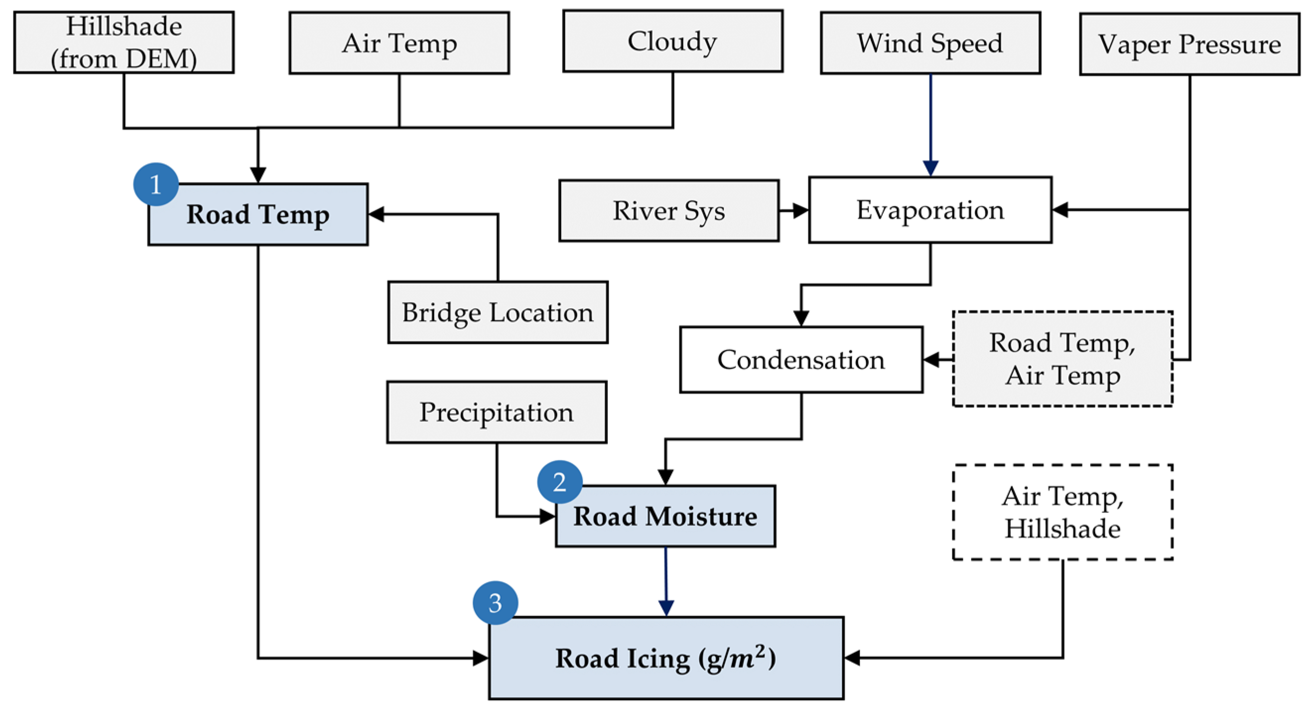
• Factors that affect road icing are mainly divided into spatial and meteorological data. Hillshade is the factor that represents spatial information and is calculated by DEM [10,11]. This factor accelerates road icing by preventing solar radiation from reaching the ground [12,13]. The main factor of meteorological data is precipitation. In particular, the freezing rain phenomenon instantaneously accelerates road icing and causes accidents [14].

• Methods

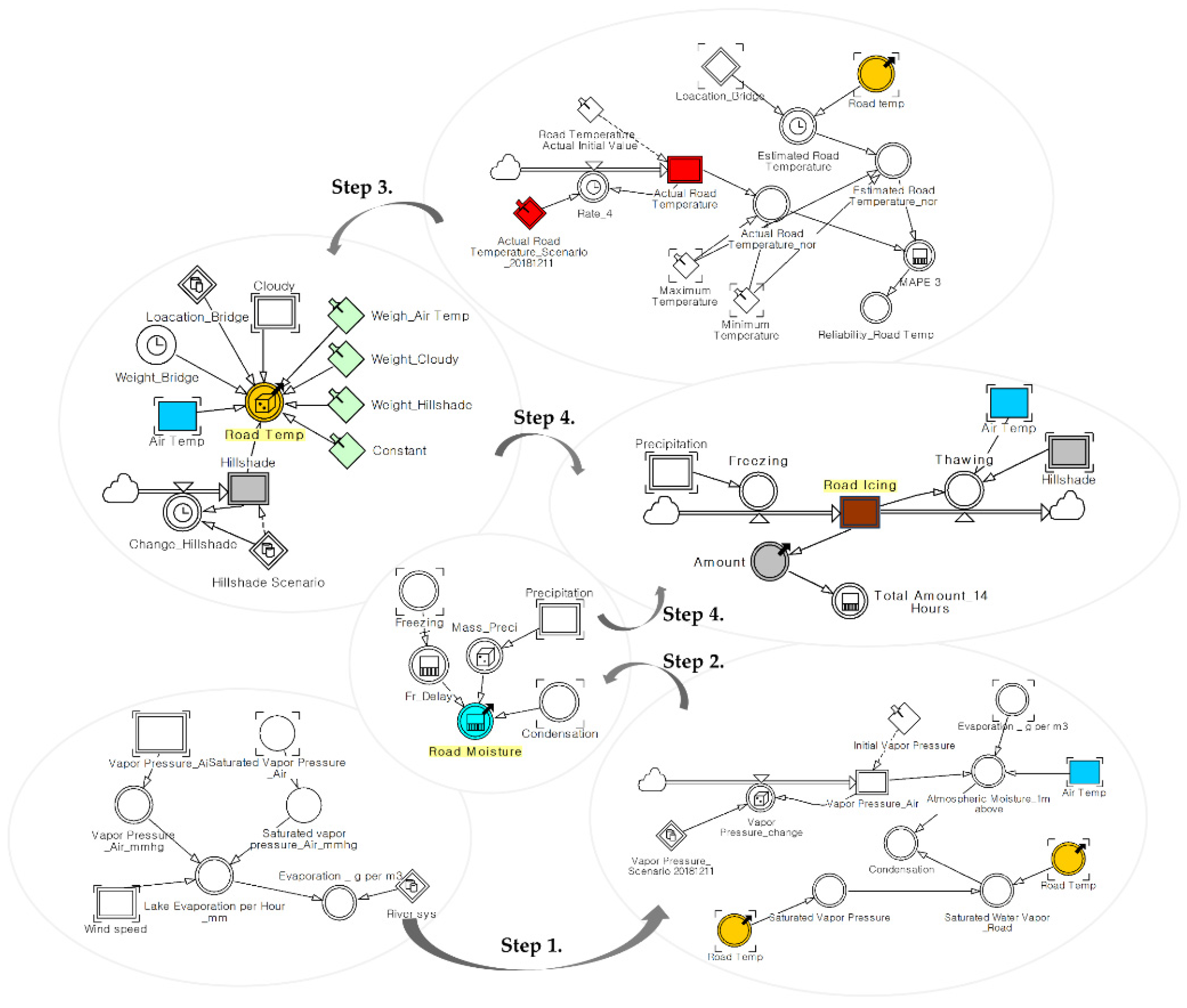
• System dynamics is a method of simulating a certain phenomenon by connecting block diagrams based on causality. In particular, it is strong in time-series expressions that are difficult to estimate for humans, while road icing is a phenomenon that continue to vary over time [15].

• Study Contributions

• The existing case studies are not complete. GIS simulation is particularly insufficient. This study addressed this insufficiency and is described later in detail.

Prior to performing road icing modeling using spatial and meteorological data, previous studies in various cases were analyzed. In general, to estimate the occurrence of road icing, the warning system is remotely controlled by monitoring the sensor information on GIS [16]. There is also a method of providing road icing information on WebGIS [17]. This method enables efficient preparation by visualizing the occurrence of road icing on the map, but has limitations in preventing them because it cannot perform prior estimation prior to occurrence [18].

Without the use of GIS, the amount of road icing can be estimated according to the weather conditions by developing a numerical model and calculating the road surface condition values according to the parameters [19]. When a numerical model is designed and meteorological data are entered, various factors can be estimated. The contents and limitations of major cases are as follows.

• Lee et al. performed numerical modeling related to road icing in Jeju Island, Korea. They estimated the air temperature and wind speed through the WRF model, but estimation of the accurate amount and location of road icing is insufficient [19].
• Kangas, Heikinheimo, and Hippi performed numerical modeling on factors related to road icing. They estimated the road surface condition and traffic condition by estimating road surface temperature, storage, and friction through the NWP model [20]. Estimation of the accurate amount and location of road icing is insufficient.
• Bezrukova, Stulov, and Khalili performed numerical modeling to estimate the occurrence of road icing. They developed a block diagram model to estimate the Ice Index through the road surface temperature, air temperature, and humidity. They could simply estimate the occurrence of road icing, and estimation of the amount and location of road icing is insufficient [21].
• Chapman, Thornes, and Bradley estimated the road surface temperature through numerical modeling from parameters. They analyzed the relationships between the “latitude, altitude, sky-view factor, screening, roughness length, road construction, traffic density, and topography” with the road surface temperature. Estimation of the accurate amount and location of road icing is insufficient [22].
• Park, Joo, and Son developed a model capable of estimating the road surface temperature by combining the Unified Model of the Korean Meteorological Administration (KMA) and the physical characteristics of the road surface. Although it is possible to estimate the road surface temperature with various factors, estimation of the amount and location of road icing is not sufficient [23].
• In other studies, road icing or related factors were also estimated mainly through simple numerical modeling. Road icing was estimated by analyzing heat conduction through the air temperature and humidity [24], measuring and analyzing road surface salinity and temperature [25], and developing short-term road icing estimation algorithms for sensors [26,27]. As in the above cases, however, estimation of the amount and location of road icing is insufficient.

These methods make it possible to systematically estimate factors related to the occurrence of road icing. Such occurrence, however, is estimated using only meteorological data, excluding spatial data, and there is no simulation stage for the occurrence location. In this study, previous insufficient cases were supplemented through system dynamics and GIS. The amount of road icing was modeled using the system dynamics theory. In addition, a section of the Honam Highway, which has a total length of 27 km, was divided into 18,583 points, and the amount and location of road icing were simulated for each point.

Numerical modeling for estimating the occurrence of road icing will make it possible to prepare for wintertime traffic accidents more efficiently if the location estimation step based on the modeling results is added [28,29]. There have been many studies on GIS simulation for disaster assessment [30]. They detect topographic hazards using GIS models [31] or analyze hazards on slopes in cold regions [32]. In addition, they evaluate and estimate the size of a hazard in high-risk areas, such as roads in hazardous ranges, using spatial data on GIS [33,34]. This method was referred to and reflected in research for the simulation of the amount and location of road icing.

After deriving implications by referring to previous studies, the amount of road icing over time was modeled by adding spatial data to meteorological data. Based on this, the amount of road icing by location was simulated using GIS. The results of estimating the amount and location of road icing through the simulation performed using appropriate scenarios can be used by government agencies (e.g., road traffic authority) as data to identify areas vulnerable to wintertime traffic accidents in advance and to prevent such traffic accidents [35].

This paper consists of five main sections. In Section 2, procedures and detailed research methods to model, simulate, and validate road icing are introduced. In addition, the study area, research data types, estimation methods, and theories are described in detail. In Section 3, the results for road surface temperature, road surface moisture, and the amount and location of road icing are presented. In Section 4, the simulation results and the actual accident points are compared and analyzed using a hypothesis testing technique. Finally, in Section 5, the results of this study are summarized and future plans to supplement shortcomings are described.

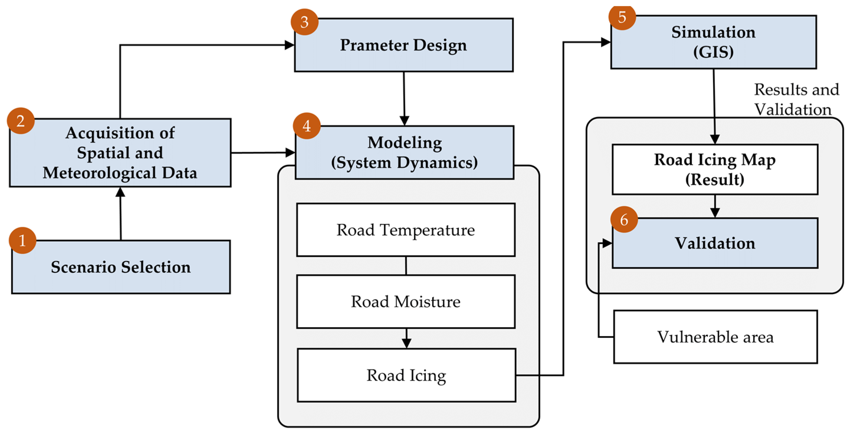
2. Materials and Methods

Research was conducted in six steps as shown in Figure 1. The first step is the selection of a scenario for model testing. The numerical results of the model were derived by selecting a scenario that shows freezing rain, which is the main cause of road icing [36]. The second step is the acquisition of spatial and meteorological data. Data that affect the generation of road icing were acquired from the Korea Meteorological Administration and topographic information-related platforms and were utilized [23]. Third, the types and values of parameters to be included in the model were designed. Fourth, modeling was performed to estimate road icing using the data and parameters selected by the scenario. It was designed to calculate road icing after calculating the road temperature and road moisture. The amount of road icing by location was then simulated by expressing the results of the modeling in GIS. Finally, it was analyzed whether road icing significantly occurred in actual areas vulnerable to traffic accidents [37].

2.1. Location of Study Area

Suncheon city in Jeollanam-do, South Korea is adjacent to the southern coast. It is associated with a large amount of rainfall, with mountainous areas formed mainly in the northern area. It also has high humidity and frequent fog formation due to the presence of many waterfront areas (e.g., lakes, rivers, and streams). Compared with nearby areas in Jeollanam-do, Suncheon had lower temperatures than the average in summer and winter. Its annual precipitation (1531.3 mm) was highest in the Jeollanam-do region. These were judged to be favorable conditions for the occurrence of road icing.

Table 2. Annual temperature in Suncheon (in summer and winter over the last ten years).

Year	Average Summer Temperature (Suncheon, °C)	Average Summer Temperature (Jeollanam-do, °C)	Average Winter Temperature (Suncheon, °C)	Average Winter Temperature (Jeollanam-do, °C)	Annual Temperature Range (Suncheon, °C)
2020	23.67	24.00	1.67	3.39	22.0
2019	23.07	23.63	3.05	4.87	20.0
2018	24.53	25.32	2.07	3.12	22.9
2017	24.23	24.60	−0.50	1.17	24.7
2016	24.15	24.60	1.80	3.39	22.4
2015	23.17	23.25	2.20	3.40	21.0
2014	22.77	23.18	0.90	2.65	22.6
2013	24.73	25.16	1.83	3.22	23.4
2012	24.27	24.51	−0.03	1.50	24.3
2011	24.03	24.00	0.13	1.34	23.9

shows the summer and winter temperatures in Suncheon and Jeollanam-do over the last ten years.

Road icing mainly occurs in roads in mountainous areas with frequent shadows, roads close to waterfront areas with high relative humidity, and roads in areas with a large amount of rainfall [1]. The Honam highway, which stretches through the mountainous areas in Suncheon, is vulnerable to road icing because shadows frequently occur in the morning hours and it has many bridges. In addition, waterfront areas are also adjacent to some sections. Therefore, a section of the Honam highway in Suncheon with these characteristics was selected as the study area. Figure 2 shows the Honam highway in Suncheon.

2.2. Acquisition of Study Data

This study sought to model and simulate road icing, and appropriate data were required for this purpose. First, data types for the model construction were selected, and actual data to perform simulation were acquired. Spatial data included the Digital Elevation Model (DEM), river system, roads, and bridges. DEM has a resolution of 5 m, and it was used through interpolation into a resolution of 1 m. Meteorological data were acquired from the Automated Synoptic Observing System (ASOS, Suncheon), and included air temperature, cloudiness, vapor pressure, wind speed, and precipitation [22,38,39].

Table 3. Major spatial data of the model and their contents.

Data Name	Data Source	Resolution	Content
DEM	Lidar Satellite	5 m (Interpolation, 1 m)	Hillshade formation
Hillshade	DEM	1 m	Scenario input Evolution algorithm train set
River System	National Spatial Data Infrastructure Portal	1 m	Scenario input
Road, Bridge	National Spatial Data Infrastructure Portal	1 m	Scenario input

and

Table 4. Major meteorological data of the model and their contents.

Data Name	Data Source	Range	Content
Air Temp	ASOS (Suncheon)	AM 00:00–PM 13:00	Scenario input Evolution algorithm train set
Cloudy	ASOS (Suncheon)	AM 00:00–PM 13:00	Scenario input Evolution algorithm train set
Vapor Pressure	ASOS (Suncheon)	AM 00:00–PM 13:00	Scenario input
Wind Speed	ASOS (Suncheon)	AM 00:00–PM 13:00	Scenario input
Precipitation	ASOS (Suncheon)	AM 00:00–PM 13:00	Scenario input

show the contents of the spatial and meteorological data. The spatial data were acquired from the 18,583 points obtained by dividing the 27 km section of the Honam Highway in Suncheon. Meteorological data were assigned to these road points by multiplying the ASOS data by a random number generated in the ∓2% range.

2.3. Scenario Selection

The weather and spatial scenarios used the data of Suncheon ASOS on 11 December 2008 as the main samples. Traffic accidents caused by road icing actually occur under various conditions, especially at night, dawn and early morning. It takes a long time to simulate all these cases, and the efficiency of simulation also decreases. Thus, it was necessary to select a representative weather situation in which road icing may occur. 11 December 2018, was the day when the largest number of freezing rain-related traffic accidents occurred during the period from 2018 to 2020 in Jeollanam-do, Korea. On that day, freezing rain phenomenon occurred, in which supercooled rain in the air at room temperature is frozen upon hitting the ground at sub-zero temperature [36]. In this study, the data of the day were set as a scenario, and the formation of road icing caused by freezing rain was modeled and simulated. The model was also verified through a comparison with actual areas vulnerable to traffic accidents.

The data of 11 December 2018 were used as a scenario because they were the latest among the freezing rain observation data of days when freezing accidents occurred, but there are a number of precipitation scenarios that can be applied to modeling.

Table 5. Past scenarios from precipitation history in winter (Suncheon, last three years).

Date	Road Surface Temperature	Air Temperature	Freezing Rain Occurrence Time	Precipitation Type
2020/12/29	Afternoon below 0 °C	Afternoon above 0 °C	PM 20:00~PM 21:00	Freezing Rain
2019/01/31	Morning below 0 °C	Morning below 0 °C	AM 3:00~PM 15:00	Snow
2018/12/16	Morning below 0 °C	Morning above 0 °C	AM 9:00~AM 15:00	Freezing Rain
2018/01/16	Morning below 0 °C	Morning above 0 °C	AM 9:00~PM 12:00	Freezing Rain
2018/01/12	Morning below 0 °C	Morning below 0 °C	AM 11:00~AM 12:00	Snow
2018/01/10	Morning below 0 °C	Morning below 0 °C	AM 3:00~PM 18:00	Snow

shows a list of such scenarios. The model and simulation are versatile for scenarios related to ordinary rain or freezing rain and can be applied to situations where the moisture in the air near waterfront areas condenses at the dew point in the cold morning even if it is not precipitation. In addition to freezing rain, the model deals with various types of precipitation in cold weather. Even when snow falls, the model can estimate the location of road icing. However, when snow is set as input, it is necessary to translate the melting time into the model when estimating the road surface moisture [40].

Figure 3 shows the trends in air and road temperatures acquired from ASOS (Suncheon) on 11 December 2018. In Figure 3b, precipitation occurred approximately from AM 9:00 to PM 12:00. Precipitation generally does not lead to road icing, but the freezing rain phenomenon occurred during the same time in Figure 3a because the air temperature was higher than 0 °C and the road temperature was lower than 0 to 1 °C.

The time range was set to 14 h from AM 12:00 to PM 13:00. As can be seen from the case analysis in the introduction, road icing traffic accidents mostly occur in the morning while air temperature reaches its peak at PM 13:00 on average. In other words, it is necessary to simulate the time period from the morning hours with low air temperature and solar radiation intensity as well as heavy traffic to PM 13:00, when frequency of road icing occurrence decreases due to high solar radiation intensity. This tendency was reflected, and the time range was set to 14 h including the morning for efficiency of the simulation.

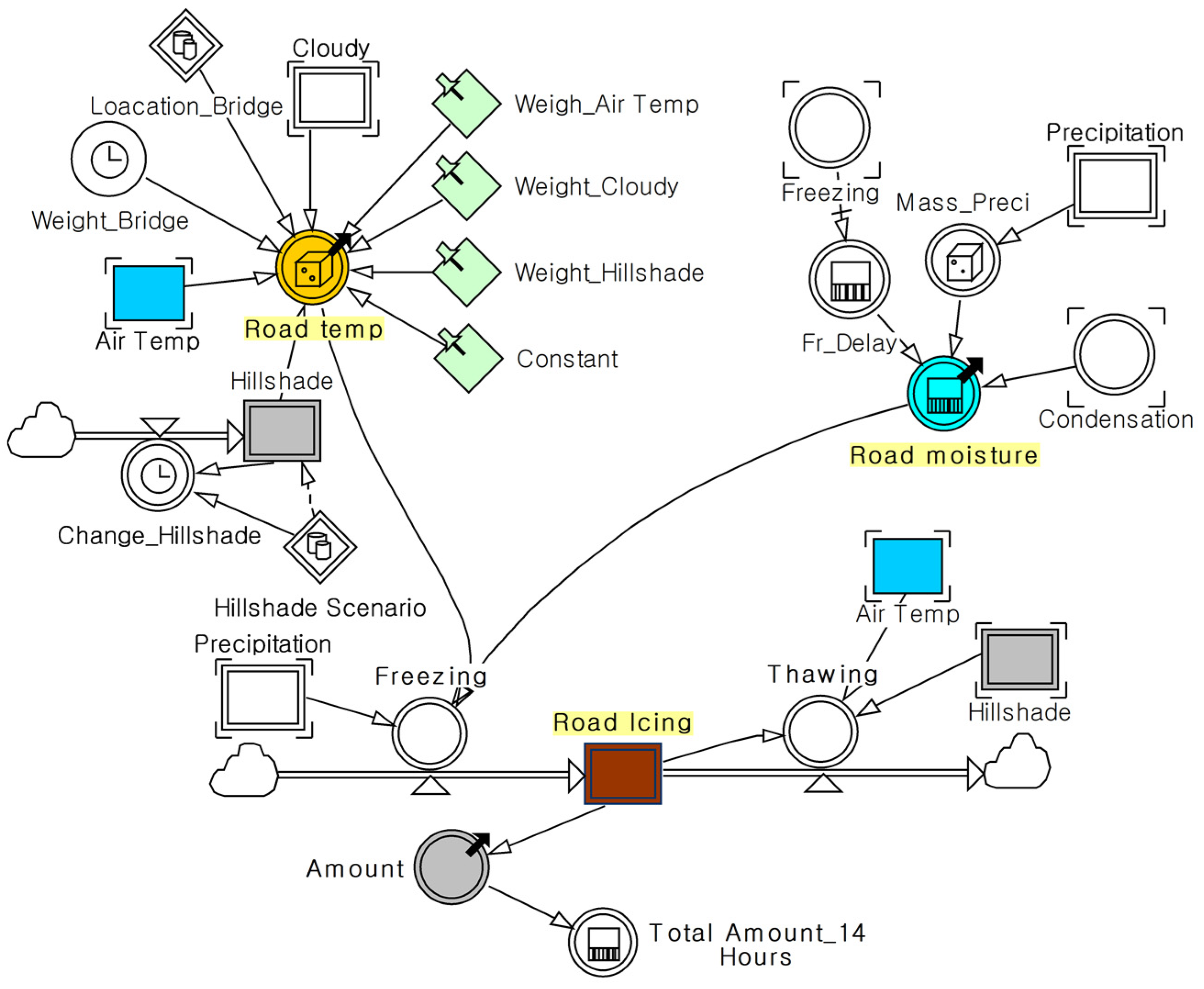
2.4. Modeling Road Icing

The system dynamics theory was used for modeling to estimate the location of road icing. This theory lists the elements that cause a specific phenomenon in a block diagram and reveals relationships among them over time [9,19]. When a natural phenomenon, such as road icing, is modeled based on the system dynamics theory, natural scientific equations can show changes in the phenomenon over time [19]. Figure 4 shows the system dynamics model structure (Please refer to the Appendix A and Appendix B).

Figure 5 shows the logic flow of data that expresses only the relationship between the input and output factors in Figure 4 and summarizes the overall flow of the model. The main output factors are (1) road temperature, (2) road moisture, and (3) road icing (g/m²). The main equations of the model are constructed to derive these three factors. The model is based on (1) road temperature and (2) road moisture and derives (3) road icing (g/m²) for GIS simulation.

The road icing model consists of various input and output factors. These factors and their information are shown in

Table 6. Main input and output factors of the model.

Factor	Category	Symbol	Value Range	Unit
Hillshade (from DEM)	Input (t = 0~13 h) Data	H	0~254	-
River System		RS	0~1	-
Bridge Location		Lb	0 or 1	-
Air Temp		Ta	−15~10	°C
Cloudy		Vc	0~10	-
Vapor Pressure		Pv	0 or more	Pa
Wind Speed		Sw	0 or more	m/s
Precipitation		P	0 or more	mm
Evaporation	Intermediate (t = 0~13 h)	E	0 or more	g/m3
Condensation		C	0 or more	g/m2
Road Temperature	Output (t = 0~13 h)	Tr	−15~10	°C
Road Moisture		Mr	0 or more	g/m2
Road Icing		RI	0 or more	g/m2

. Each symbol is the expression method of the corresponding factor in the equation in the numerical model, and the numerical expression represents the range and unit of values. This information was used, and the derivation process and equations for (1) road temperature, (2) road moisture, and (3) road icing (g/m²), which are the main output factors, were explained at the end of Section 2. All the factors have a range of 14 h from AM 00:00 to PM 13:00.

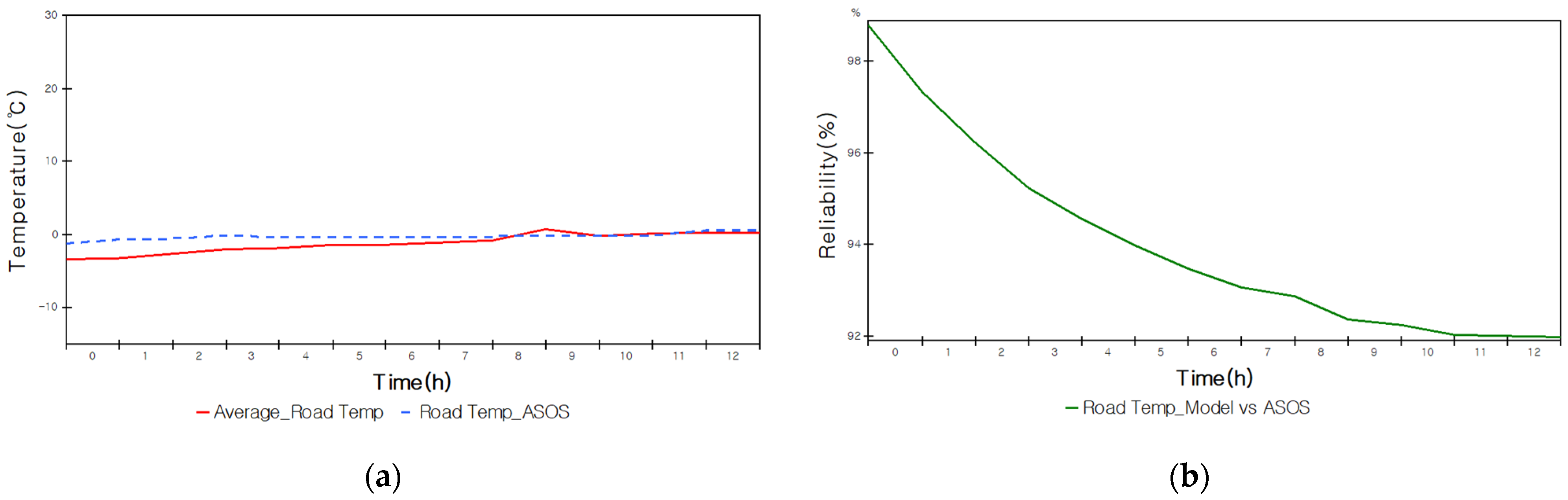
2.4.1. Road Temperature

Road temperature is one of the important factors in road icing occurrence. This is because the moisture present on roads freezes at sub-zero temperatures [41]. For traditional road temperature calculation, a large number of input factors are required, including “weather variables, such as solar radiation energy, air temperature, atmospheric pressure, and wind, as well as thermal characteristic values according to the material of the road surface” [23]. This, however, is not appropriate due to the nature of simulation, which must exhibit the highest efficiency with limited input. In this study, a method of producing the highest estimation performance with a small number of input factors through an evolution algorithm was devised [42,43,44,45,46]. The input factors used were hillshade, air temperature, cloudiness, and bridge location as shown in Figure 5 and Table 3.

A multiple linear regression equation was constructed using these four factors as shown in Equation (1), and the parameters (A, B, C, D, and E) were optimized using the evolution algorithm [42,43,44,45,46]. In the case of parameter D, the initial value was set to −1 to −2 over time through literature survey because its optimization through the evolution algorithm was estimated to be insignificant.

$${\mathrm{T}}_{\mathrm{r}}=\mathrm{f}\left({\mathrm{T}}_{\mathrm{a}}{, \mathrm{H}, \mathrm{V}}_{\mathrm{c}}{,\mathrm{L}}_{\mathrm{b}}\right){=\mathrm{A}*\mathrm{T}}_{\mathrm{a}}+\mathrm{B}*\mathrm{H}*\mathrm{C}*\left\{\left({\mathrm{V}}_{\mathrm{c}} - 10\right)*-1\right\}{+\mathrm{D}*\mathrm{L}}_{\mathrm{b}}+\mathrm{E}$$

(1)

The air temperature in Equation (1) is an integral value obtained by adding the differential value over time to the initial value (T_a)_t=0. The air temperature is calculated using Equation (2).

$${\mathrm{T}}_{\mathrm{a}}=\int {{(\mathrm{T}}_{\mathrm{a}}{}^{’})}_{\mathrm{t}}{\mathrm{dt}+(\mathrm{T}}_{\mathrm{a}}{)}_{\mathrm{t}=0}$$

(2)

Hillshade in Equation (1) is an integral value obtained by adding the differential value over time to the initial value H_t=0. Hillshade is calculated using Equation (3).

$$\mathrm{H}=\int {\mathrm{H}}^{’}{}_{\mathrm{t}}{\mathrm{dt}+\mathrm{H}}_{\mathrm{t}=0}$$

(3)

Cloudiness in Equation (1) is an integral value obtained by adding the differential value over time to the initial value (V_c)_t=0. Cloudiness is calculated using Equation (4).

$${\mathrm{V}}_{\mathrm{c}}=\int {({\mathrm{V}}_{\mathrm{c}}{}^{’})}_{\mathrm{t}}\mathrm{dt}+{\left({\mathrm{V}}_{\mathrm{c}}\right)}_{\mathrm{t}=0}$$

(4)

The evolution algorithm mainly goes through the processes of initial set setting, crossbreeding or mutation, fitness calculation, roulette model, and termination condition checking. In this study, the termination condition of the evolution algorithm is when the fitness function F(t) has the minimum value [42,46]. F(t) is the formula for the mean absolute percentage error value within modeling and expressed as Equation (5). At is the actual value and Ft is the estimated value.

$$\mathrm{F}\left(\mathrm{t}\right)=\frac{100\%}{\mathrm{n}}{\displaystyle \sum }_{\mathrm{t}=0}^{\mathrm{t}=13}\left|\frac{{\mathrm{A}}_{\mathrm{t}}-{ \mathrm{F}}_{\mathrm{t}}}{{\mathrm{A}}_{\mathrm{t}}}\right|$$

(5)

Genes whose fitness was calculated are selected through the roulette function. When selecting three chromosomes to select offspring, the global optimal solution cannot be found if simply three chromosomes with the highest fitness are selected because it damages chromosome diversity. The roulette function, a concept of probabilistic chromosome selection, was used to address this problem. It is a concept of probabilistically selecting certain chromosomes based on P(t) defined as shown in Equation (6). In Equation (6), N is the number of chromosomes and F(t) is a function for obtaining fitness [42].

$$\mathrm{P}\left(\mathrm{t}\right)=\frac{\mathrm{F}\left(\mathrm{t}\right)}{{\sum }_{\mathrm{i}}^{\mathrm{N}}\mathrm{F}\left(\mathrm{t}\right)}$$

(6)

The standard for estimating the minimum value of the fitness function F(t) for the genes selected using the roulette function is when the value of F(t) is repeated within 0.000000001, which is the set value of minimum convergence. Figure 6 shows the schematic of the evolution algorithm used for parameter optimization. The process of forming chromosome groups Cc(t) and Cm(t) through crossbreeding and mutation of the first three parent chromosomes, the fitness function, the roulette function, and the process of determining the termination condition are shown [42,46]. For parameter training, a total of 98 train data of Suncheon, Jeollanam-do from 12 to 18 December 2018 were used. While training was performed using the train data, the optimized parameters of A, B, C, D, and E were derived when the termination condition was satisfied.

The road temperature on 11 December 2018, which is the test set, could be obtained by applying the optimized parameters, and it was compared with the meteorological data (ground surface temperature) of the actual ASOS for verification. For the comparative verification, the mean absolute percentage error of Equation (7), which was also used for the fitness function, and the reliability of Equation (8) were used.

$$\mathrm{MAPE}=\frac{100\%}{\mathrm{n}}{\displaystyle \sum }_{\mathrm{t}=0}^{\mathrm{t}=13}\left|\frac{{\mathrm{A}}_{\mathrm{t}}{ - \mathrm{F}}_{\mathrm{t}}}{{\mathrm{A}}_{\mathrm{t}}}\right|$$

(7)

$$\mathrm{Reliability}(\%)=\left(1 - \mathrm{MAPE}\right)*100(\%)$$

(8)

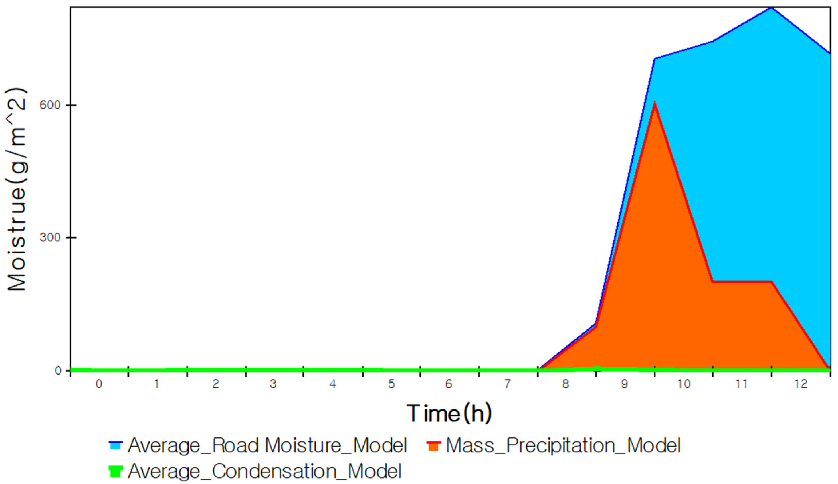
2.4.2. Road Moisture

Road moisture is an important factor in the formation of road icing along with road temperature [47]. When moisture forms on a road, a decrease in road temperature below zero forms road icing. There are two cases in which moisture is formed on a road as follows. Based on these, two input factors were derived. The input factors that affect the formation of road moisture are precipitation (mass) and condensation.

• Case (1) when water is collected on a road by precipitation (Precipitation)
• Case (2) when water vapor condenses on a road as the road temperature drops below the dew point (Condensation)

The formula to obtain road moisture using precipitation (mass) and condensation is as follows. C is the condensation, MoP is the mass of precipitation, and Fr is the amount of freezing water. The road moisture formed by precipitation and condensation freezes and decreases.

$${\mathrm{M}}_{\mathrm{r}}={\displaystyle \sum }_{\mathrm{t}=0}^{\mathrm{t}=13}{(\mathrm{MoP}+\mathrm{C} - \mathrm{Fr})}_{\mathrm{t}}$$

(9)

The mass of precipitation in Equation (9) is the actual mass of precipitation per hour on an area of 1 m². This is expressed in Equation (10). P is the precipitation (mm) and MoP is the mass of precipitation (g/m²).

$$\mathrm{MoP}\left({\mathrm{g}/\mathrm{m}}^2\right)=\frac{{\mathsf{\pi } \mathrm{r}}^2\mathrm{P}}{10}$$

(10)

The condensation in Equation (9) is calculated using the equation between the current amount of water vapor in the atmosphere and the amount of saturated water vapor on the road. The temperature of the water vapor contained in the atmosphere drops below the dew point near the road surface, and condensation occurs. The content on condensation is shown in Equation (11). C is the condensation (g/m²), E is the evaporation (g/m³), V is the amount of vapor (g/m³), and Vs is the amount of saturated water vapor (g/m³).

$$\mathrm{C}={\displaystyle \sum }_{\mathrm{t}=0}^{\mathrm{t}=13}{(\mathrm{E}+\mathrm{V} - \mathrm{V}}_{\mathrm{s}})$$

(11)

For the evaporation in Equation (11), Dalton’s law formula based on Dalton’s aerodynamic was used. It is a theory that the movement of water molecules from a free surface is proportional to the vapor pressure gradient in the vertical direction [48]. This is expressed in Equation (12). E is the amount of evaporation from the reservoir, e_s is the saturated vapor pressure at the air temperature (mmHg), P_v is the actual vapor pressure at the air temperature (mmHg), and Sw is the wind speed (m/s) at a height of 2 m from the water surface (m/s) [48].

$$\mathrm{E}=0{.345*(\mathrm{e}}_{\mathrm{s}}{ - \mathrm{P}}_{\mathrm{v}})*(0.5+0{.54\mathrm{S}}_{\mathrm{w}})$$

(12)

The amount of vapor (V) in Equation (11) is obtained using Equation (13). P_v is the vapor pressure and T_a is the air temperature [49].

$$\mathrm{V}=217*\frac{{\mathrm{P}}_{\mathrm{v}}}{{\mathrm{T}}_{\mathrm{a}}+273.15}$$

(13)

P_v in Equation (12) is the vapor pressure, and it is entered into the model as an integral value to which the differential values over time are added. This is expressed in Equation (14). The integrated value Pv was obtained by adding the amount of change per time to the initial value (P_v)_t=0.

$${\mathrm{P}}_{\mathrm{v}}=\int {{(\mathrm{P}}_{\mathrm{v}}{}^{’})}_{\mathrm{t}}{\mathrm{dt}+(\mathrm{P}}_{\mathrm{v}}{)}_{\mathrm{t}=0}$$

(14)

S_w in Equation (12) is the wind speed. It is entered into the model as an integral value to which the differential values over time are added. This is expressed in Equation (15). The integrated value S_w was obtained by adding the amount of change per time to the initial value (S_w)_t=0.

$${\mathrm{S}}_{\mathrm{w}}=\int {{(\mathrm{S}}_{\mathrm{w}}{}^{’})}_{\mathrm{t}}{\mathrm{dt}+(\mathrm{S}}_{\mathrm{w}}{)}_{\mathrm{t}=0}$$

(15)

2.4.3. Road Icing

When road temperature and road moisture are derived, road icing per hour can be calculated [47]. The road icing model is basically expressed as an integral value for the amount of change in freezing and thawing [50,51]. For freezing, the road temperature and road moisture calculated above are involved. In the presence of road moisture, the amount of change in freezing occurs if the road temperature satisfies certain conditions. For thawing, Hillshade and air temperature are involved. A higher value of Hillshade means larger exposure to sun energy [29,52]. In addition, when road moisture freezes, it is affected by the air temperature because it rises to the top due to a reduction in density, and more thawing occurs as its value increases. This is expressed in Equation (16). Ft is the amount of change in freezing over time and Th_t is the amount of change in thawing over time.

$$\mathrm{RI}=\int {(\mathrm{F}}_{\mathrm{t}}{}^{’}{ - \mathrm{Th}}_{\mathrm{t}}{}^{’})\mathrm{dt}$$

(16)

Contents on the amount of change in freezing, Ft, are shown in Equation (17). Ft is a function of the road temperature (T_r), road moisture (M_r), and precipitation (P). The value of Ft is determined according to the conditions of the precipitation and road temperature. In the presence of precipitation, road moisture freezes when road temperature is below 1 °C. In the absence of precipitation, road moisture freezes when road temperature is below 0 °C.

$${\mathrm{F}}_{\mathrm{t}}=\mathrm{f}{\left({\mathrm{T}}_{\mathrm{r}}{,\mathrm{M}}_{\mathrm{r}},\mathrm{P}\right)}_{\mathrm{t}}=\{\begin{array}{c}{\mathrm{M}}_{\mathrm{r}}*\frac{{-\mathrm{T}}_{\mathrm{r}}+1}{5}{, (\mathrm{if} \mathrm{P} > 0 \mathrm{and} \mathrm{T}}_{\mathrm{r}} < 1)\\ {\mathrm{M}}_{\mathrm{r}}*\frac{{-\mathrm{T}}_{\mathrm{r}}+1}{5}{, (\mathrm{if} \mathrm{P}=0 \mathrm{and} \mathrm{T}}_{\mathrm{r}} < 0)\end{array}$$

(17)

Contents on the amount of change in thawing (Th_t) are shown in Equation (18). Th_t is a function of Hillshade (H) and air temperature (Ta). Th_t is determined according to the conditions of the air temperature. If air temperature is higher than 0 °C, thawing occurs in proportion to the amount of Hillshade (0 to 254). If it is lower than 0 °C, no thawing occurs.

$${\mathrm{Th}}_{\mathrm{t}}=\mathrm{f}{\left(\mathrm{RI}{,\mathrm{H}, \mathrm{T}}_{\mathrm{a}}\right)}_{\mathrm{t}}=\{\begin{array}{c}{\mathrm{RI}}_{\mathrm{t}-1}*\frac{\mathrm{H}}{254}{, (\mathrm{T}}_{\mathrm{a}} > 0)\\ {0, (\mathrm{T}}_{\mathrm{a}} \le 0)\end{array}$$

(18)

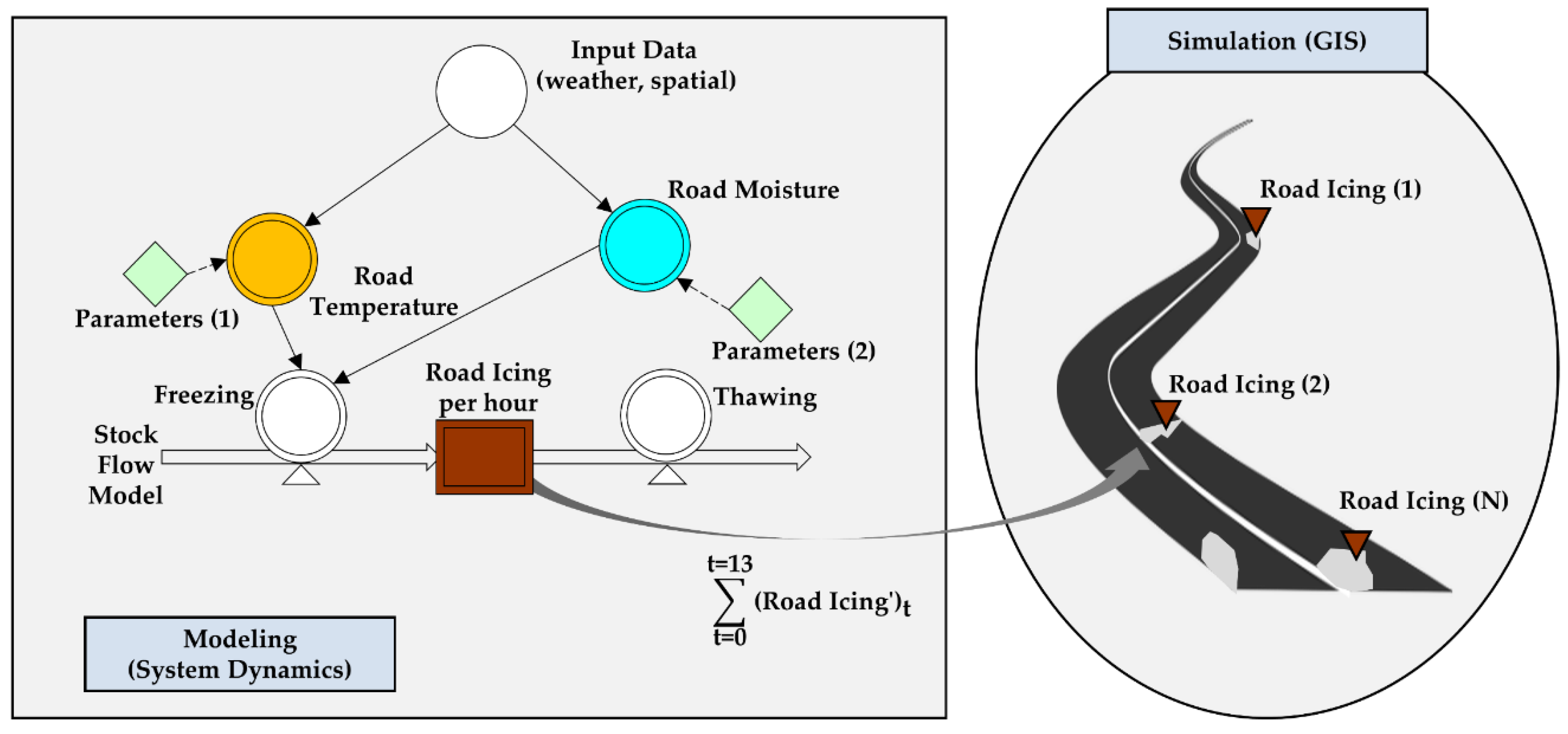
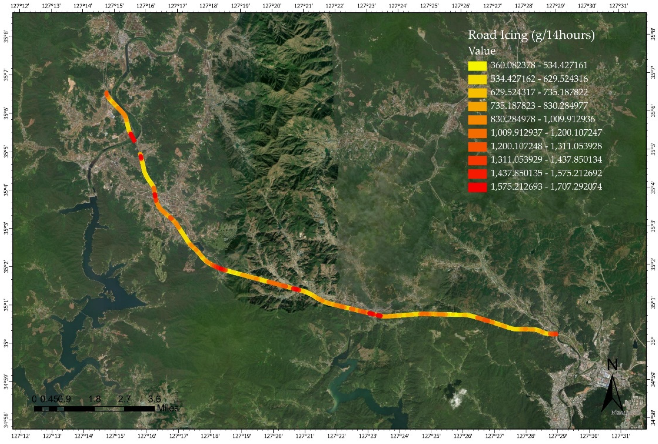
2.5. GIS Simulation of Road Icing

The amount of road icing generated per hour is modeled for all the sections of the target highway in the unit of 1 m². The total amount and location of road icing were estimated and simulated on GIS by adding all generated values per hour from AM 00:00 to PM 13:00. The total amount of road icing is calculated using Equation (19). RI_t=0..13 is expressed in g/m² and displayed in GIS, making it possible to estimate sections with a number of road icing.

$${\mathrm{RI}}_{\mathrm{t}=\mathrm{0..13}}={\displaystyle \sum }_{\mathrm{t}=0}^{\mathrm{t}=13}{\mathrm{FR}}_{\mathrm{t}}$$

(19)

Road icing per hour is calculated by the Stock Flow Model as shown in the modeling section of Figure 7. Calculated road icing is superimposed by hour on GIS, and the total amount for 14 h, RI_t=0..₁₃, is obtained for each section of the highway.

3. Results

Road temperature and road moisture were modeled for the Honam Highway in Suncheon. Road icing was subsequently modeled, and the amount and location of road icing were simulated on GIS. The modeling results for road temperature and road moisture are shown in Section 3.1, while the results of modeling and simulating the amount and location of road icing are presented in Section 3.2.

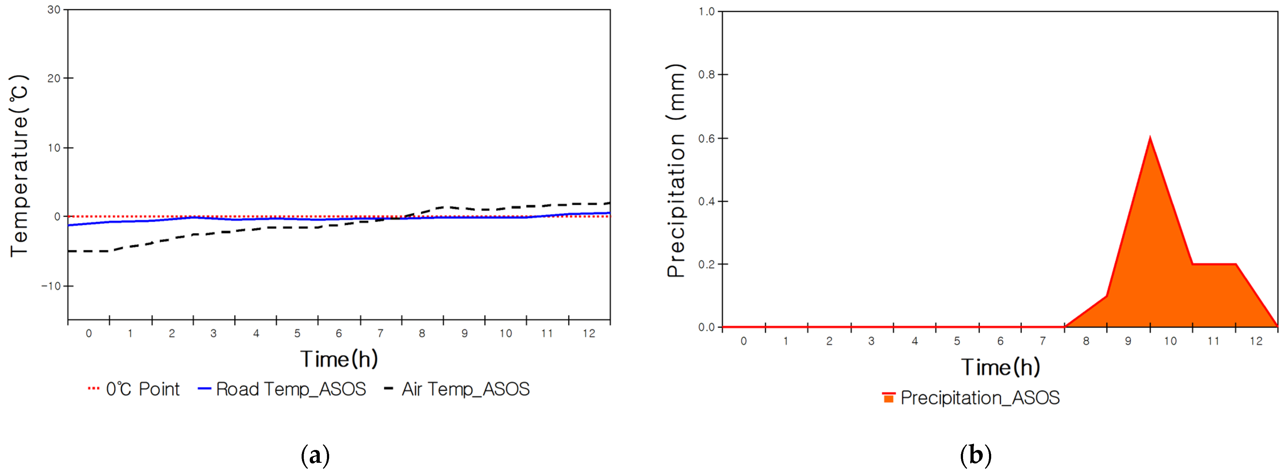
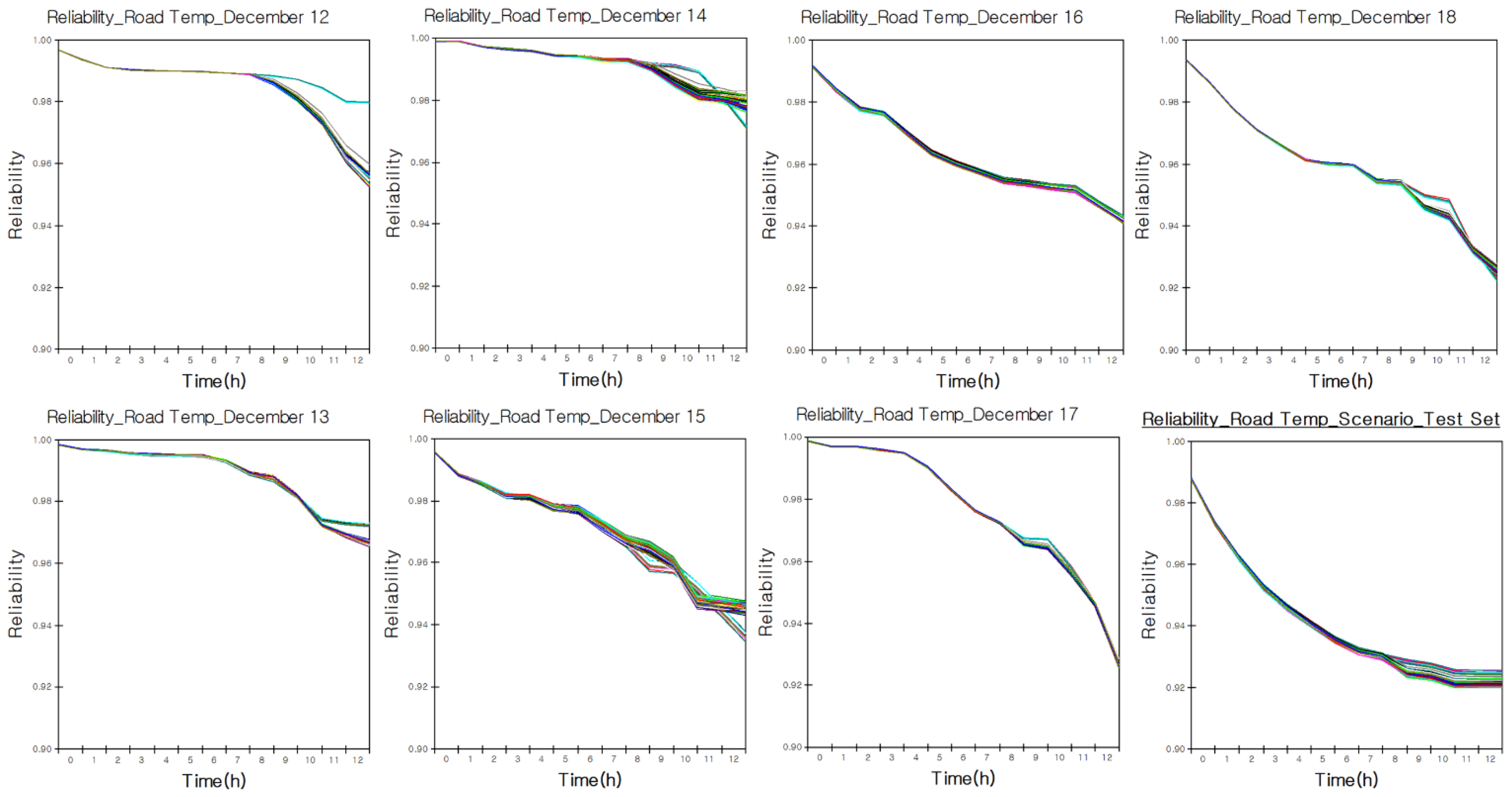
3.1. Modeling Results for Road Temperature and Moisture

Road temperature and road moisture are important factors in calculating the amount of road icing generated per hour. Road temperature was trained using the evolution algorithm. The results of the corresponding training set and test set are shown in Figure 8. December 12th to 18th exhibited a degree of training of 95% on average. The accuracy of the test set was found to be 91.88%. This was estimated to be a significant value because it far exceeded the target value of 80% set in this study.

Figure 9 shows the results of the road temperature. The average of the estimated values at 18,583 road points was calculated and expressed as a graph along with the actual road temperature values acquired from ASOS in Figure 9a. The reliability between the estimated and actual values was calculated over time and expressed in Figure 9b. As confirmed in Figure 8 above, reliability was calculated at 91.88%.

Figure 10 shows the results of the road moisture. Average road moisture for 18,583 road points and the precipitation and condensation value that generate it were expressed. Road moisture significantly increased from AM 9:00 at which point it began to rain and a total amount of more than 700 g was maintained until PM 13:00. The average condensation value was low because there were not many waterfront areas adjacent to the highway, but high values were observed in some sections.

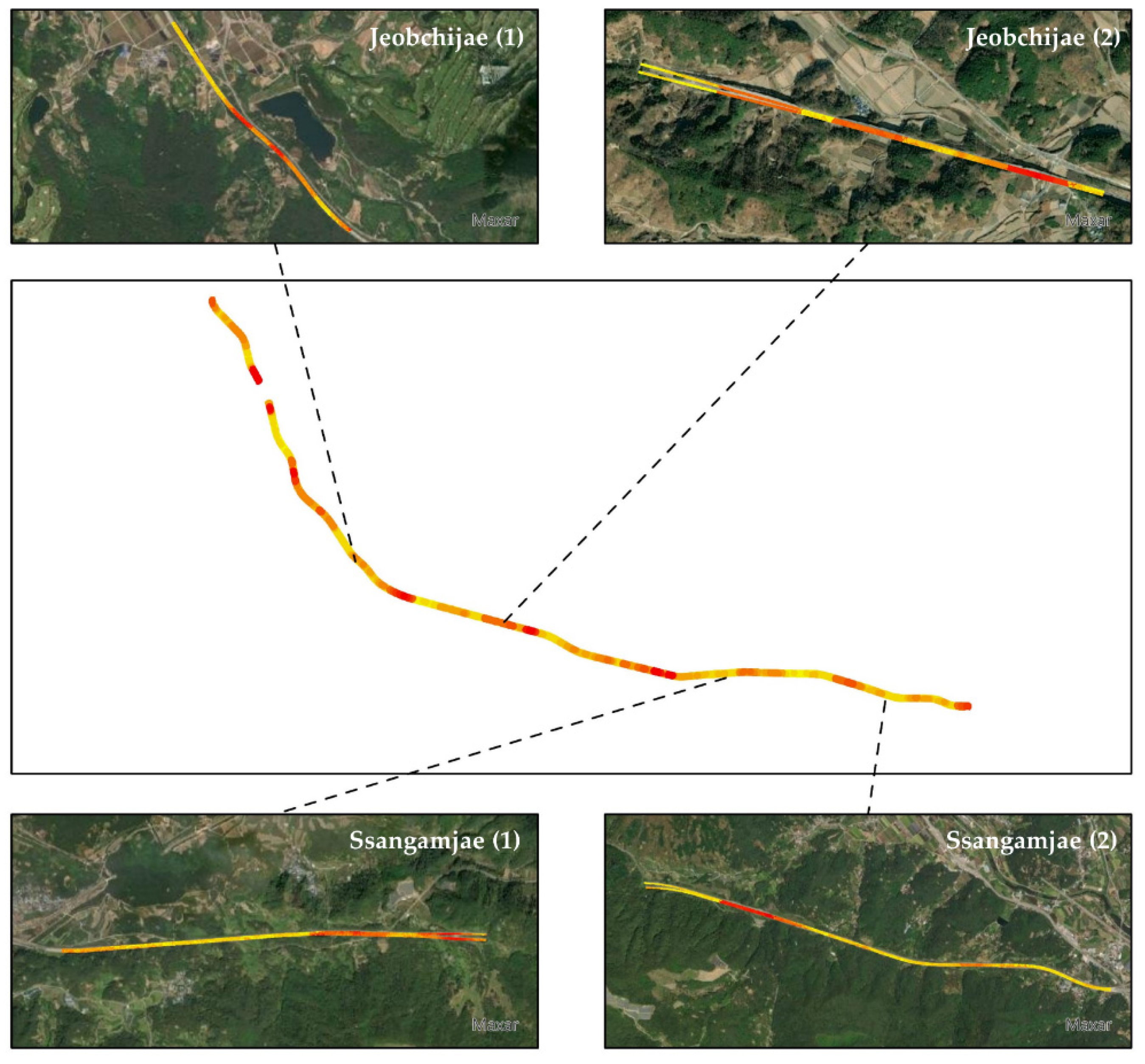
3.2. Modeling and Simulation Results for Road Icing

The amount of road icing, which is the final result, was derived based on the results of road temperature and road moisture obtained above. Figure 11 shows a graph on the amount of road icing. It exhibited a maximum value of 213.62 g/m² at noon and then decreased. Thawing and freezing happened simultaneously, and the amount changed over time due to the factors that cause road icing.

The total amount of road icing was simulated on GIS [53] by reflecting the results of Figure 11. The results are shown in Figure 12. These are the results of simulating the total amount of road icing that occurred for 14 h on the Honam highway in Suncheon by location. The generation of 360.082 to 1707.292 road icing was observed by location.

4. Discussion

In this study, the road temperature and road moisture per hour were modeled, and the amount of road icing generated per hour was obtained through these two factors. The obtained amount of road icing per hour was added, and the sum of the amount for 14 h was simulated by location on GIS. The road moisture formed a relationship with the freezing road according to the road temperature. The freezing temperature of the road moisture ranged from 1 to −10 °C depending on the presence of precipitation. In addition, as the temperature decreased, road icing formed at a higher rate per unit time.

As can be seen from the cases in the introduction section, previous studies on road icing estimation use simple numerical modeling to estimate the road surface temperature or weather conditions. In this study, however, the amount and location of road icing were estimated as shown in Figure 12.

Table 7. Comparison of the results of this study with previous cases.

Case	Road Temperature		Road Moisture		Road Icing		GIS simulation
	Estimation	Form	Estimation	Form	Estimation	Form	Performance	Form
Case ① [19]	√	Occurrence/non-occurrence	–	–	–	–	–	–
Case ② [20]	√	Value	–	Index	√	Index	–	–
Case ③ [21]	√	Value	–	Index	√	Index	–	–
Case ④ [22]	√	Value	–	–	–	–	–	–
Case ⑤ [23]	√	Value	–	–	–	–	–	–
This study	√	Value, location information	√	Value, location information	√	Value, location information	√	GIS layer

√ performed, – not performed.

below compares the results of this study with data of previous cases. All studies basically estimate road surface temperature, but they do not estimate road moisture and road icing or estimate at the level of an index. In this study, both road temperature and road moisture were estimated in numerical values along with the location information, and the amount and location of road icing were simulated on GIS.

To verify the validity of the model, road icing occurrence tendencies in vulnerable sections with freezing traffic accident records were analyzed. Four sections were analyzed as shown in the table below, and these are part of the Honam highway in Suncheon. The names of each section were Jeobchijae (1), Jeobchijae (2), Ssangamjae (1), and Ssangamjae (2). The four sections belong to line 25 of the Honam highway in Jeollanam-do, Korea. Each of them has one to four freezing accident records attributed to morning shading [54]. The related contents are shown in

Table 8. List of sections vulnerable to freezing traffic accidents in Honam highway in Suncheon.

Section Name	Management Number	Line	Freezing Accidents (Morning)	Regional Characteristics	Minimum Temperature
Jeobchijae (1)	287	Honam highway line 25	3 to 4	Morning shading	−3~0 °C
Jeobchijae (2)	288	Honam highway line 25	1 to 2	Morning shading	−3~0 °C
Ssangamjae (1)	289	Honam highway line 25	1 to 2	Morning shading	−3~0 °C
Ssangamjae (2)	290	Honam highway line 25	1 to 2	Morning shading	−3~0 °C

.

Figure 13 shows the locations of each section vulnerable to freezing traffic accidents [53]. The corresponding zone was expressed by extracting the related areas and dividing the road icing into 1 to 10 steps.

For all four sections, it was set in the scenario that freezing rain occurred from AM 9:00 to AM12:00. The monitoring period was set to the period between AM 10:00 and AM 13:00 because the generation of road icing in the model was examined one hour after the occurrence of freezing rain. As for the model validity verification method, the upper tailed test method that uses the p-value after establishing the null and alternative hypotheses was adopted [55]. The p-value is a test static probability value for judging that the null hypothesis is wrong in the research model, i.e., a probability that a certain research hypothesis (alternative hypothesis) exhibits a type 1 error (error that the null hypothesis is wrong). If the research hypothesis is tested at the 95% confidence level, 0.05 (α, 5%) is set as the significance level. If the p-value is lower than 0.05 (significance level, i.e., the probability that a type 1 error is allowed), the null hypothesis is rejected and the research hypothesis is adopted. The null and alternative hypotheses were established as follows, and the adoption of the alternative hypothesis was confirmed by calculating the P-value of each section and comparing it with 0.05 (significance level) [56].

• H0: (null hypothesis) the model does not generate thin ice in the vulnerable area (RI < 3 g/m³).
• H1: (alternative hypothesis) the model generates thin ice in the vulnerable area (RI >= 3 g/m³).

For null and alternative hypothesis testing, the p-value was calculated by conducting the upper tailed test on the road icing formed under conditions below 1 °C after the occurrence of freezing rain. The formula to obtain the Z-score that standardized the performance value, X, is shown in Equation (20). X is the variable related to the amount of freezing roads generated, μ is the average amount, σ is the standard deviation, and n is the number of variables [56].

$$\mathrm{Z}=\frac{\mathrm{X} - \mathsf{\mu }}{\frac{\mathsf{\sigma }}{\sqrt{\mathrm{n}}}}$$

(20)

When the p-value was calculated using the Z-score value in

Table 9. Upper tailed test through the p-value in the sections vulnerable to freezing traffic accidents.

Section Name	Freezing Rain	Average Amount (Freezing Rain)	Z-Score	p-Value (One-Tailed)	Test Results
Jeobchijae (1)	AM9:00~PM12:00	135.77 (g/m2)	13.61	0.000010 (<0.05)	H1 adoption
Jeobchijae (2)	AM9:00~PM12:00	208.37 (g/m2)	2.01	0.022216 (<0.05)	H1 adoption
Ssangamjae (1)	AM9:00~PM12:00	142.56 (g/m2)	8.23	0.000010 (<0.05)	H1 adoption
Ssangamjae (1)	AM9:00~PM12:00	152.81 (g/m2)	2.08	0.018763 (<0.05)	H1 adoption

, the p-value was lower than 0.05 in the four sections, so the null hypothesis was rejected and the alternative hypothesis was adopted. In the upper tailed test results, the model estimated the amount of road icing generated in the vulnerable sections where freezing accidents occurred, thereby verifying the validity of the model.

5. Conclusions

In this study, modeling was performed through the system dynamics theory to estimate the amount and location of road icing, and the results were simulated on the geographic information system (GIS). In the system dynamics model, the amount of road icing per unit area (1 m²) was modeled by combining block diagrams in the causal order. In this model applied per unit area, the amount and location of road icing for 14 h were simulated by calculating numerical values differently depending on the specific values (spatial and meteorological data) of each road section.

The upper tailed test through the p-value was then conducted in vulnerable areas where actual freezing traffic accidents occurred, and the alternative hypothesis that the model properly simulates the generation of thin ice in vulnerable areas was adopted. Through this hypothesis testing, it could be estimated that the model properly simulates the actual occurrence of road icing. Research was conducted on estimating the occurrence of road icing through modeling in vulnerable areas, but freezing traffic accidents are caused by many factors, such as the presence of slopes, signals, and curves, as well as a simple degree of freezing on the road. In other words, although the model estimates the amount and location of road icing, it has limitations in accurately selecting places vulnerable to traffic accidents due to the omission of additional vulnerability factors. If calculation is performed by adding the factors described above, such as slopes, signals, and curves, it will be possible to estimate traffic accident vulnerability more accurately. The results can also be compared with the data of actual points where traffic accidents occurred.

In the future, it is necessary to conduct further research on vulnerability by superimposing these factors in the form of a layer on GIS or calculating them along with parameters in the system dynamics theory. This study is significant, as the location and amount of road icing are simulated prior to risk evaluation. In addition, the results of this study can be useful data for government agencies (e.g., road traffic authority) in managing traffic accidents caused by road icing. If factors are reinforced and more accurate vulnerability assessment is performed in the future, it will be possible to reduce manpower wasted for surveys on vulnerable sections by selecting points where damage from road icing is expected in advance. It will also be possible to efficiently implement structural and non-structural measures at more accurate points.

References

1. Cary, L. Black Ice; Vintage: New York, NY, USA, 2010. [Google Scholar]
2. Lee, S.J. Traffic Accident Article (Case1). Available online: http://news.tvchosun.com/site/data/html_dir/2020/01/06/2020010690068.html (accessed on 6 January 2020).
3. Jung, S.H. Traffic Accident Article (Case2). Available online: http://www.joynews24.com/view/1231389 (accessed on 26 December 2019).
4. Kim, M.I. Traffic Accident Article (Case3). Available online: https://www.segye.com/newsView/20191129511652?OutUrl=naver (accessed on 29 November 2019).
5. Authority, R.T. Traffic Accident Analysis System. Available online: http://taas.koroad.or.kr/web/shp/adi/initBasisPurps.do?menuId=WEB_KMP_IID_IID_PAB (accessed on 1 January 2020).
6. Jones, K.; Eylander, J. Vertical variation of ice loads from freezing rain. Cold Reg. Sci. Technol. 2017, 143, 126–136. [Google Scholar] [CrossRef]
7. Yan, Q.; Li, B.; Zhang, Y.; Yan, J.; Zhang, C. Numerical Investigation of Heat-Insulating Layers in a Cold Region Tunnel, Taking into Account Airflow and Heat Transfer. Appl. Sci. 2017, 7, 679. [Google Scholar] [CrossRef] [Green Version]
8. Qiu, P.; Li, P.; Hu, J.; Liu, Y. Modeling Seepage Flow and Spatial Variability of Soil Thermal Conductivity during Artificial Ground Freezing for Tunnel Excavation. Appl. Sci. 2021, 11, 6275. [Google Scholar] [CrossRef]
9. Kim, C.H. System Dynamics; pybook: Seoul, Korea, 2021. [Google Scholar]
10. Choi, B.-G.; Kim, J.-S. Extraction of road surface freezing section using GIS. J. Korean Soc. Geospat. Inf. Syst. 2005, 13, 19–25. [Google Scholar]
11. Lee, H.S. Analyses on sunshine influence and surface freezing section of road using GIS. J. Korean Soc. Surv. Geod. Photogramm. Cartogr. 2005, 23, 293–301. [Google Scholar]
12. Del Vecchio, M.C.; Ceppi, A.; Corbari, C.; Ravazzani, G.; Mancini, M.; Spada, F.; Maggioni, E.; Perotto, A.; Salerno, R. A Study of an Algorithm for the Surface Temperature Forecast: From Road Ice Risk to Farmland Application. Appl. Sci. 2020, 10, 4952. [Google Scholar] [CrossRef]
13. Mirzanamadi, R.; Hagentoft, C.-E.; Johansson, P. Numerical Investigation of Harvesting Solar Energy and Anti-Icing Road Surfaces Using a Hydronic Heating Pavement and Borehole Thermal Energy Storage. Energies 2018, 11, 3443. [Google Scholar] [CrossRef] [Green Version]
14. Toms, B.A.; Basara, J.B.; Hong, Y. Usage of Existing Meteorological Data Networks for Parameterized Road Ice Formation Modeling. J. Appl. Meteorol. Climatol. 2017, 56, 1959–1976. [Google Scholar] [CrossRef]
15. Sterman, J. Business Dynamics; McGrawHill: New York, NY, USA, 2000. [Google Scholar]
16. Liu, T.; Wang, N.; Yu, H.; Basara, J.; Hong, Y.E.; Bukkapatnam, S. Black Ice Detection and Road Closure Control System for Oklahoma (Fhwa-Ok-14-01 2239). Oklahoma Department of Transportation: Oklahoma City, OK, USA, 2014. [Google Scholar]
17. Li, S.; Xiong, C.; Ou, Z. A Web GIS for sea ice information and an ice service archive. Trans. GIS 2011, 15, 189–211. [Google Scholar] [CrossRef]
18. Liu, T.; Pan, Q.; Sanchez, J.; Sun, S.; Wang, N.; Yu, H. Prototype Decision Support System for Black Ice Detection and Road Closure Control. IEEE Intell. Transp. Syst. Mag. 2017, 9, 91–102. [Google Scholar] [CrossRef]
19. Lee, Y.-M.; Oh, S.-Y.; Lee, S.-J. A study on prediction of road freezing in Jeju. J. Environ. Sci. Int. 2018, 27, 531–541. [Google Scholar] [CrossRef]
20. Kangas, M.; Heikinheimo, M.; Hippi, M. RoadSurf: A modelling system for predicting road weather and road surface conditions. Meteorol. Appl. 2015, 22, 544–553. [Google Scholar] [CrossRef]
21. Bezrukova, N.; Stulov, E.; Khalili, M. A model for road icing forecast and control. In Proceedings of the Proceedings SIRWEC, Turin, Italy, 25–27 March 2006; pp. 50–57. [Google Scholar]
22. Chapman, L.; Thornes, J.E.; Bradley, A.V. Modelling of road surface temperature from a geographical parameter database. Part 2: Numerical. Meteorol. Appl. 2001, 8, 421–436. [Google Scholar] [CrossRef]
23. Park, M.-S.; Joo, S.J.; Son, Y.T. Development of road surface temperature prediction model using the Unified Model output (UM-Road). Atmosphere 2014, 24, 471–479. [Google Scholar] [CrossRef] [Green Version]
24. Sass, B.H. A Numerical Model for Prediction of Road Temperature and Ice. J. Appl. Meteorol. 1992, 31, 1499–1506. [Google Scholar] [CrossRef] [Green Version]
25. Xu, H.; Zheng, J.; Li, P.; Wang, Q. Road icing forecasting and detecting system. In AIP Conference Proceedings; AIP Publishing LLC: Melville, NY, USA, 2017; p. 020089. [Google Scholar]
26. Troiano, A.; Pasero, E.; Mesin, L. New system for detecting road ice formation. IEEE Trans. Instrum. Meas. 2010, 60, 1091–1101. [Google Scholar] [CrossRef] [Green Version]
27. Teke, M.; Duran, F. The design and implementation of road condition warning system for drivers. Meas. Control 2019, 52, 985–994. [Google Scholar] [CrossRef] [Green Version]
28. Wilson, D. Using machine learning to predict car accident risk. Proc. Medium-Geospat. Artif. Intell. 2018. [Google Scholar]
29. Shao, J.; Lister, P. The prediction of road surface state and simulation of the shading effect. Bound.—Layer Meteorol. 1995, 73, 411–419. [Google Scholar] [CrossRef]
30. Dyras, I.; Serafin-Rek, D. The application of GIS technology for precipitation mapping. Meteorol. Appl. 2005, 12, 69–75. [Google Scholar] [CrossRef]
31. Brini, I.; Alexakis, D.D.; Kalaitzidis, C. Linking Soil Erosion Modeling to Landscape Patterns and Geomorphometry: An Application in Crete, Greece. Appl. Sci. 2021, 11, 5684. [Google Scholar] [CrossRef]
32. Shin, Y.; Choi, J.C.; Quinteros, S.; Svendsen, I.; L’Heureux, J.-S.; Seong, J. Evaluation and Monitoring of Slope Stability in Cold Region: Case Study of Man-Made Slope at Øysand, Norway. Appl. Sci. 2020, 10, 4136. [Google Scholar] [CrossRef]
33. Liu, H.; Wang, X.; Liao, X.; Sun, J.; Zhang, S. Rockfall Investigation and Hazard Assessment from Nang County to Jiacha County in Tibet. Appl. Sci. 2019, 10, 247. [Google Scholar] [CrossRef] [Green Version]
34. Mousavi Tayebi, S.A.; Moussavi Tayyebi, S.; Pastor, M. Depth-Integrated Two-Phase Modeling of Two Real Cases: A Comparison between r.avaflow and GeoFlow-SPH Codes. Appl. Sci. 2021, 11, 5751. [Google Scholar] [CrossRef]
35. Liu, B.; Lv, Y.; Guo, Z. A Study of Road Surface Ice Prediction Based on Highway Operations and Safety. In ICTIS 2013: Improving Multimodal Transportation Systems-Information, Safety, and Integration, Proceedings of the Second International Conference on Transportation Information and Safety, Wuhan, China, 29 June 29–2 July 2013; American Society of Civil Engineers: Reston, VA, USA, 2013; pp. 1244–1250. [Google Scholar]
36. Zerr, R.J. Freezing rain: An observational and theoretical study. J. Appl. Meteorol. 1997, 36, 1647–1661. [Google Scholar] [CrossRef]
37. Almoshaogeh, M.; Abdulrehman, R.; Haider, H.; Alharbi, F.; Jamal, A.; Alarifi, S.; Shafiquzzaman, M. Traffic Accident Risk Assessment Framework for Qassim, Saudi Arabia: Evaluating the Impact of Speed Cameras. Appl. Sci. 2021, 11, 6682. [Google Scholar] [CrossRef]
38. Kang, J.-E.; Kim, J.-J. Assessment of Observation Environments of Automated Synoptic Observing Systems Using GIS and WMO Meteorological Observation Guidelines. Korean J. Remote Sens. 2020, 36, 693–706. [Google Scholar]
39. Administration, K.M. KMA Weather Data Service—Open MET Data Portal. Available online: https://data.kma.go.kr/cmmn/main.do (accessed on 11 December 2020).
40. Salimi, S.; Nassiri, S.; Bayat, A.; Halliday, D. Lateral coefficient of friction for characterizing winter road conditions. Can. J. Civ. Eng. 2016, 43, 73–83. [Google Scholar] [CrossRef]
41. Park, K.; Kim, Y.; Lee, K.; Kim, D. Development of a Shallow-Depth Soil Temperature Estimation Model Based on Air Temperatures and Soil Water Contents in a Permafrost Area. Appl. Sci. 2020, 10, 1058. [Google Scholar] [CrossRef] [Green Version]
42. Holland, J.H. Genetic algorithms and adaptation. In Adaptive Control of Ill-Defined Systems; Springer: Berlin/Heidelberg, Germany, 1984; pp. 317–333. [Google Scholar]
43. Lin, C.-M.; Liu, H.-Y.; Tseng, K.-Y.; Lin, S.-F. Heating, Ventilation, and Air Conditioning System Optimization Control Strategy Involving Fan Coil Unit Temperature Control. Appl. Sci. 2019, 9, 2391. [Google Scholar] [CrossRef] [Green Version]
44. Zhang, L.; Li, C.; Wu, Y.; Zhang, K.; Shi, H. Hybrid Prediction Model of the Temperature Field of a Motorized Spindle. Appl. Sci. 2017, 7, 1091. [Google Scholar] [CrossRef] [Green Version]
45. Ge, Z.; Li, J.; Duan, Y.; Yang, Z.; Xie, Z. Thermodynamic Performance Analyses and Optimization of Dual-Loop Organic Rankine Cycles for Internal Combustion Engine Waste Heat Recovery. Appl. Sci. 2019, 9, 680. [Google Scholar] [CrossRef] [Green Version]
46. Gorni, D.; Visioli, A. Genetic Algorithms Based Reference Signal Determination for Temperature Control of Residential Buildings. Appl. Sci. 2018, 8, 2129. [Google Scholar] [CrossRef] [Green Version]
47. Karlsson, M. Prediction of hoar-frost by use of a Road Weather Information System. Meteorol. Appl. 2001, 8, 95–105. [Google Scholar] [CrossRef]
48. Silberberg, M.S.M.S. Chemistry: The Molecular Nature of Matter and Change; McGraw-Hill: Boston, MA, USA, 2009. [Google Scholar]
49. Bejan, A. Advanced Engineering Thermodynamics; John Wiley & Sons: Hoboken, NJ, USA, 2016. [Google Scholar]
50. Ishida, T.; Pen, K.; Tanaka, Y.; Kashimura, K.; Iwaki, I. Numerical Simulation of Early Age Cracking of Reinforced Concrete Bridge Decks with a Full-3D Multiscale and Multi-Chemo-Physical Integrated Analysis. Appl. Sci. 2018, 8, 394. [Google Scholar] [CrossRef] [Green Version]
51. Pradhan, N.R.; Downer, C.W.; Marchenko, S. Catchment Hydrological Modeling with Soil Thermal Dynamics during Seasonal Freeze-Thaw Cycles. Water 2019, 11, 116. [Google Scholar] [CrossRef] [Green Version]
52. Bonanno, R.; Loglisci, N.; Cavalletto, S.; Cassardo, C. Analysis of Different Freezing/Thawing Parameterizations using the UTOPIA Model. Water 2010, 2, 468–483. [Google Scholar] [CrossRef] [Green Version]
53. World_Imagery. Available online: https://services.arcgisonline.com/ArcGIS/rest/services/World_Imagery/MapServer (accessed on 20 January 2020).
54. Corporation, K.E. A supplementary management card for the ice vulnerability management section (management chart, May 22, 2020). 2020. [Google Scholar]
55. Hogg, R.V.; McKean, J.; Craig, A.T. Introduction to mathematical statistics; Pearson Education: London, UK, 2005. [Google Scholar]
56. Raftery, A.E.; Gilks, W.; Richardson, S.; Spiegelhalter, D. Hypothesis testing and model. Markov Chain Monte Carlo Pract. 1995, 1, 165–187. [Google Scholar]
Figure 1. Summary of the methodology used in this research, including data, modeling, simulation, validation.
Applsci 11 08537 g001
Figure 2. Honam highway in Suncheon.
Applsci 11 08537 g002
Figure 3. Freezing rain analysis for scenario feasibility: (a) road (and air) temperature of ASOS (Suncheon, 2018/12/11); (b) precipitation of ASOS (Suncheon, 2018/12/11).
Applsci 11 08537 g003
Figure 4. System dynamics model for predicting road icing.
Applsci 11 08537 g004
Figure 5. Logic flow of data composing the system dynamics model.
Applsci 11 08537 g005
Figure 6. Schematic of the evolution algorithm for parameter optimization.
Applsci 11 08537 g006
Figure 7. Schematic diagram of the road icing simulation.
Applsci 11 08537 g007
Figure 8. Training and test results of the evolution algorithm for the road temperature.
Applsci 11 08537 g008
Figure 9. Graph of road temperature per hour and reliability: (a) road temperature comparison graph (model and ASOS); (b) road temperature estimation reliability graph (model and ASOS).
Applsci 11 08537 g009
Figure 10. Road moisture estimation results.
Applsci 11 08537 g010
Figure 11. Road icing estimation results.
Applsci 11 08537 g011
Figure 12. Simulation result of occurrence and location of road icing.
Applsci 11 08537 g012
Figure 13. Map of the sections vulnerable to freezing traffic accidents in Honam highway in Suncheon (Jeobchijae1, 2, Ssangamjae1, 2).
Applsci 11 08537 g013