3.1. Methodology Overview
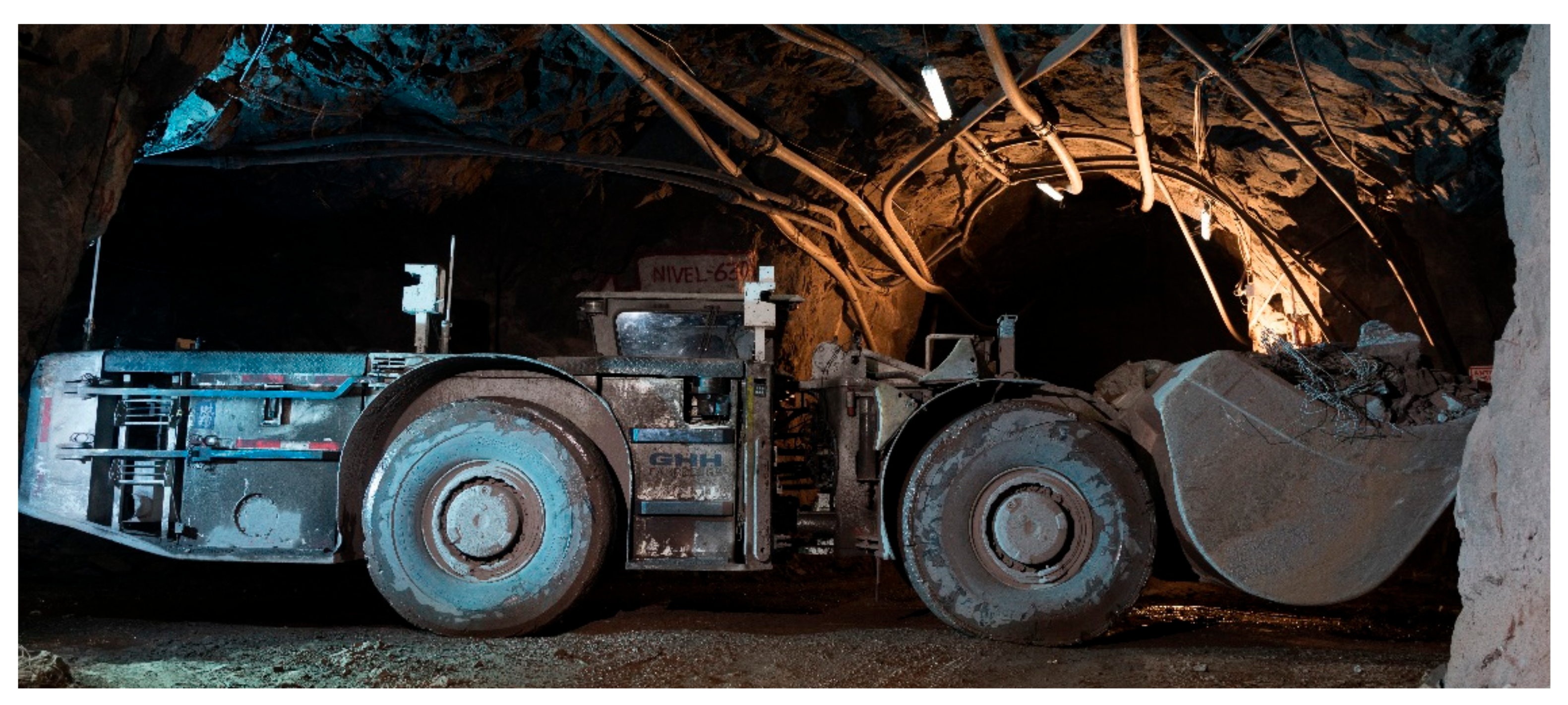
The hardware used in this work included a full-scale LHD machine (a GHH LF11H with 11-ton tramming capacity and hydraulic powertrain) retrofitted with two 2D laser scanners (SICK LMS511), encoders in all joints (IFM RN7012), pressure sensors along the bucket’s tilt and the boom’s lift hydraulic lines (manufacturer specific, 600 bar), and an onboard industrial computer (Advantech ARK-2151-59AIE) (see
Figure 1). All components are of industrial grade, suitable for the rigorous environment of underground mining, and readily available as off-the-shelf components used widely in a broad range of commercial applications. In order to better integrate the system with commercial autonomous navigation solutions for LHDs, which only use 2D scanners, 3D laser scanners were not used in the current version of the proposed system. The software implementation was performed using ROS as the central middleware [
28], CABSL library [
29] for state-machine codification, and ROS actions to interface with the main processing function in each state. The system was initially developed and tested in a simulated environment using Gazebo [
30].
An autonomous loading routine can be thought of as a sequence of several steps that perform specific actions, as presented in the diagram of
Figure 2. There, rock pile identification is the process of finding the draw point’s location and status (whether it is suited for loading or not). Positioning refers to orienting the LHD machine to ensure that a forward thrust will end in a collision with the rock pile. Charging is the step that considers lowering the bucket and accelerating towards the pile. Excavation is the machine control that performs the digging action. Pull back comprises the backward motion of the vehicle and bucket shake. Finally, Payload weighing estimates the amount of ore loaded. Most of the mentioned steps could fail due to the highly variable environment in underground mining. It is possible that the onboard sensors fail to find the rock pile accurately or that the machine positioning cannot avoid colliding with a tunnel wall. The collision between the machine and the rock pile might not be detected, and the LHD’s bucket could become stuck during excavation. In any of these cases, human assistance would be required to overcome the problematic situation. In fact, human interaction with automated mobile machines for mining operations is needed in the state-of-the-art systems, at the very least to supervise a fleet of machines. Since large-scale operations have a fleet of vehicles, it is common for one or more operators to supervise and assist multiple semi-autonomous machinery, as each machine does not require constant attention. For these reasons, in our view, it is imperative that this human interaction is considered at the design stage of the autonomous loading system and, thus, included in the formulation of the agent’s behavior.
Figure 6 shows the proposed state machine for the autonomous loading process with the human in the loop. There are two assistance states: positioning assistance allows the operator to take control of the machine to position it in front of the rock pile, while loading assistance provides the operator with full control of the LHD to perform the remaining parts of the loading maneuver up until payload weighing, which is needed to record the performance of the task. The positioning assistance is called either when the rock pile identification cannot characterize the rock or when positioning is not able to place the LHD to start the charging procedure, while loading assistance is called when the charging, the excavation, or the pull back procedures cannot be successfully completed.
3.2. Environment Modeling and Rock Pile Identification
Of the six steps of the autonomous loading routine, the first one, rock pile identification, is the one that most strongly relies on the processing of data acquired from the environment. The aim of this step is to find the location and status of the draw point accurately, in real time, and without the need of extra steps or delays. This means that the LHD is required to continue moving while scanning the pile. The characterization of the rock pile is performed through integration of consecutive laser scans from the frontal 2D LIDAR sensor mounted on the LHD. The integration of the laser scans relies on a LIDAR-based odometry method [
31], and the output of the machine’s inclinometer data, which is filtered and integrated in the local coordinate frame in order to benefit from the natural tilting of the LHD while moving across uneven terrain. The aforementioned odometry method consists of an adaptive frame rate modification of the range-flow based odometry (RF2O) [
32]. While RF2O computes displacement by comparing two scans, using the “range flow constraint equation”, the adaptive frame rate implements a control over the processing frequency, increasing it at higher machine speeds.
A block diagram for the pile identification step is presented in
Figure 7. The LIDAR odometry enables the integration of 2D laser scans into a 3D point cloud of the environment. Then, the rock pile is segmented, and its features are computed (center, limits, and slope).
A conceptual diagram of the complete pile identification process is shown in
Figure 8. The succession of images (a, b, and c) illustrates how the integration is carried out. For each new scan (colored circles), the data is registered in an accumulated point cloud, using the computed odometry. It is important to note that the whole process must be executed in real time without stopping, or even slowing down, the LHD. Moreover, the fact that the LIDAR reaches the bottom of the pile from a long distance away, because it is tilted down 2.5 degrees, results in the point cloud having very low density, all of which increases the complexity of the problem.
Once enough scans have been integrated, the rock pile is segmented using the normal vectors of the surface, a curvature filter, and neighbors count in a small radius. The normal vectors provide information about the points belonging to the walls or to the pile (normal ny is negative on the left wall, near zero on the pile, and positive on the right wall). The curvature provides a rotation-invariant description of the points, which can be used for further segmenting the pile. Finally, neighbor counts provide information valuable for rejecting outliers (points that are isolated from all others). Once a pile is segmented successfully, its mean slope is estimated and is used to classify the status of the pile: a too shallow slope indicates there is not enough ore to perform a loading, and a too steep slope signals the presence of a tunnel wall instead of a rock pile, or even a rock pile in a “hang-up” state, a condition that can arise in certain underground mining methods, such as block caving, in which the fragmented rock stops flowing, generating an unstable and hazardous condition. The determination of the status of the pile is performed by a simple thresholding of its slope.
For clarity purposes, the described algorithm for segmenting and characterizing the pile is detailed in
Figure 9.
Besides the pile status, the locations of the horizontal bounds are needed for the next step of the loading routine, the machine positioning. The left (
EL) and right (
ER) limits of the rock pile are required to be able to direct the machine without colliding with the tunnel walls. Using the information available from the pile segmentation algorithm, the limits are estimated as
EL = max_y, and
ER = min_y (see definitions in
Figure 9).
The normal vectors of the points provide valuable information for segmenting the pile, as shown in
Figure 10. In this figure, low values of the normal component
ny are colored in blue, while high values are colored in red.
Oversized rock detection can also be performed in this identification step; however, the description of the functionality is outside the scope of this paper (see, for example, the detection system described in [
33]).
If the identification of the rock pile has not finished by the time the LHD is closer than a certain predetermined distance to the pile (in the experiments, a threshold of 15 m was used), a transition to the positioning assistance state is forced in the behavior state machine from
Figure 6. In the experiments, a threshold of 15 m was used as the predetermined distance. This value was deemed sufficient for the LHD to successfully achieve the following positioning in front of the rock pile. The overall loading routine is, nevertheless, not sensitive to small variations of the selected parameter, and its value should be selected based on the particular conditions of the operating environment.
3.3. Positioning and Charging
After the draw point location and status have been determined, the loading routine continues with the positioning of the machine. Here, the LHD is continued to be driven forward using a “guidance” algorithm [
34] until the machine’s reference point (in this case its central articulation joint) is at a set distance from the center of the pile (computed as the center of gravity of the segmented points). Once this distance is met, small corrections to the steering angle are issued to ensure that the projected path lands within the limits of the rock pile. Finally, the bucket is lowered until a tight contact with the ground is achieved. A block diagram of this process is shown in
Figure 11.
The projected path for the machine aligning procedure (see
Figure 12) is computed using the LHD’s kinematic equations, reported in several previous publications, such as [
35]:
where
is the pose of the LHD,
is the linear speed,
is the steering angle of the LHD’s pivot,
is the steering speed of the LHD’s pivot,
is the length from the LHD’s pivot to the rear wheel axis, and
is the length from the LHD’s pivot to the front wheel axis.
Since the next step of the autonomous loading routine, the charging against the rock pile, does not involve steering commands, a fixed steering angle (constant
γ,
ω = 0) can be considered, which simplifies the model:
where
is a constant value that depends on the LHD dimensions and the fixed steering angle. Equation (3) shows that an LHD charging against a rock pile will follow a circular trajectory, characterized by a center (
) and a curvature radius (
). Because the
rock pile identification step computed the left (
) and right (
) pile edges, the problem of determining if the LHD will collide with the rock pile simplifies to checking if the line between
and
intersects with both the circular path of the left and right sides of the LHD.
Figure 12 shows a diagram of the described scenario.
The solution for the intersection between a circle and a line segment is well known in the common literature and it involves computing the following discriminant value:
where
is the vector going from
to
and
is the vector going from
to
. If
results in a negative value, then the infinite line defined by the points
and
never intersects the given circular path. On the other hand, if
is positive, a solution exists. Let
and
be solutions to the intersection between the infinite line defined by
and
and the circle of center
and curvature radius
:
then, if
or
, the circular path intersects the segment
. Otherwise, if
, the circular path passes to the right of the segment
. If none of the previous conditions is met, then the path passes to the left of segment
.
The above process is executed for the circular paths defined by the left and right side of the LHD. If one of them does not intersect the pile, the steering angle is adjusted in the appropriate direction until both paths land within the rock pile limits. During this steering adjustment, a simple collision check is computed periodically over a bounding box for each body of the LHD.
Figure 13 shows a diagram of the collision check for the front body of the LHD. A bounding box is defined for the front body. Then, vectors going from the bottom left corner to the top left corner (
) and to the bottom right corner (
) are defined. In order to check if point
of the detected tunnel wall is inside the bounding box (and hence causing a collision), the following condition is evaluated:
where
is the vector going from the bottom left corner of the bounding box to point
. If the condition is true, then point
is inside the collision bounding box.
Once the machine’s steering angle has been adjusted so that its projected path lands within the rock pile limits, the bucket of the LHD is lowered using the tilt hydraulic cylinder. The tilt cylinder is commanded to extend until the pressure in its hydraulic line rises over a predefined threshold, signaling a tight contact between the bucket tip and the ground. An example from full-scale experimental data is shown in
Figure 14, where a threshold of 23 bars was selected.
If the above positioning process is not completed within a predefined time limit (in the experiments, a threshold of 30 s was used), an operator assistance request is generated, effectively putting the system in the positioning assistance state from
Figure 6. Otherwise, once the vehicle is in position and with the bucket down, it is commanded to drive forward in first gear. The transition to the excavation phase occurs as the collision with the rock pile is detected by a patented method that analyzes the machine’s transmission pressure (engine load) and a skidding factor, estimated from the LIDAR odometry and the machine’s tachometer data [
18]. A block diagram is shown in
Figure 15.
The skidding estimator from
Figure 15 computes the skidding factor with the following formula:
where
is the skidding factor;
is the speed measured from the machine’s tachometer;
is the speed estimated with the LIDAR-based odometry method mentioned in
Section 3.2., and
is a normalizing factor, computed as the maximum between
and
in a fixed time window.
Simultaneously, the collision detector module monitors the pressure of the hydrostatic transmission system (for the used LF11H LHD, this variable correlates with the engine’s power output). If either the skidding factor or the transmission pressure rises above a predefined threshold, a collision detection event is flagged.
Figure 16 shows a plot of the skid factor and the transmission pressure signals, alongside the tilt command, for a teleoperated loading maneuver. The collision with the rock pile happens just before the human operator activates the tilt command. As mentioned above, a significant rise in the transmission pressure, and of the skidding factor, can be seen at that point. Extensive analysis of experimental data, such as shown in
Figure 16, led to transmission pressure threshold to be set at 300 bar, and the skidding factor threshold at 0.5.
If a collision detection is not generated within a predefined time limit (in the experiments, a threshold of 10 s was used), an operator assistance request is issued, forcing the system into loading assistance state from
Figure 6.
3.4. Excavation Algorithm
The excavation algorithm is based on the techniques used by experienced human operators from block caving, panel caving and sublevel stoping operations (which are the most common type of underground operations in Chile). From a control theory point of view, the proposed method acts as a traction controller during the excavation process. A diagram is shown in
Figure 17. The pregenerated commands is simply a module in charge of generating precomputed commands for the pedal and tilt signals. These commands are similar to the commands observed during manual operation. Specifically, the acceleration pedal is maintained at a constant output value and the bucket tilt is intermittently activated in the form of a ramp function. A ramp function was only selected in order to have an extra parameter, although a parameter sensibility analysis could not be performed in the full-scale experiments due to time constrains. The traction controller acts on the lift command in order to suppress wheel skidding, a variable that is estimated from Equation (7), as explained in
Section 3.3. In practice, a simple “on/off” controller was implemented, where the lift command was set at the maximum value if the estimated skidding factor raised over a predefined threshold. This choice was made to keep the methods simple in favor of achieving a validation of the complete system.
The implementation of the excavation method was carried out using a two-state machine. In the first state, called
, a fixed acceleration and a ramp-shaped bucket tilt command are selected. In the second state, called
, the fixed acceleration command persists, and wheel skidding is analyzed. If the wheel-skidding factor rises above a predefined threshold, the boom lift command of the machine is activated in order to compensate for it. A machine-specific option, named “full RPM”, is also activated during this state. This option forces the engine to maximize its power output, providing additional penetration force. Formally, the following equations apply for the machine commands:
where
,
, and
are predefined constant values;
is the start time of state
, and
is the skidding factor. As for the output commands,
is the signal sent to the machine’s internal control unit that regulates acceleration (similar to the signal sent when pressing the physical pedal in the machine’s cabin),
is the signal sent to retract (positive values) or extend (negative values) the cylinder that controls the movement of the bucket of the LHD machine, and
is the signal that commands the “boom” cylinder of the machine, that is, the arm that can lift (positive values) or lower (negative values) the bucket. Finally, the
signal is, as mentioned, a machine-specific command that forces the engine’s RPM to the maximum, temporarily increasing the force of the hydraulic mechanism. It should be noted that analysis and correction of wheel skidding is only performed during the
state. This decision was made based on the empirical observation that wheel skidding is much less likely to occur during bucket retraction and the fact that activating the lift cylinder effectively reduces the power available for the tilt hydraulics. In
Figure 18, a flow chart of the excavation process is presented, where EP represents engine power (a variable observed, in this case, through the transmission pressure of the machine).
Both states,
(tilt state) and
(push state), have upper and lower bounds to their execution time, so it is guaranteed that their execution alternates during the excavation. Besides the time limit of
, the system can transition back to
if the hydrostatic transmission pressure (or, more generally, the engine power output) climbs over a threshold value, meaning that the resistive force from the rock pile is too large, and the bucket is not able to penetrate further without a scooping motion. This alternation between states continues until any of the following stop criteria are met: the bucket is fully retracted, the bucket is lifted over a maximum angle, or the machine has advanced further than a maximum displacement value. This method was patented as reported in [
36]. For clarity purposes, a pseudo code of the described algorithm is shown in
Figure 19.
Table 1 shows the value of the parameters used for the full-scale validation experiments reported in
Section 4. The numerical values were selected based on operation data.
In the case that the described excavation process is not completed within a predefined time limit (in the experiments, a threshold of 30 s was used), an operator assistance request is generated, thus putting the system in the loading assistance state from
Figure 6.


