Abstract
In the 4D world of three-dimensional (3D) space plus time that we live in, there is a vast blue ocean in the spatio-temporal domain of micrometers and milliseconds that has never been accessed even with the most advanced measurement technology, and it is expected to be full of various non-equilibrium phenomena. In this paper, we review recent advances in synchrotron hard X-ray tomography we have made that can be used to explore the 4D frontier.
1. Introduction
While telescopes and microscopes have been used for more than 400 years to unravel the mysteries of the universe and matter, the ability to take continuous images beyond the limits of the human eye is a relatively recent development, dating back only about 150 years. Since the advent of the charge-coupled device (CCD) image sensor in 1970 [1], digital cameras have gradually replaced film cameras, and this digitalization has dramatically accelerated the speed of continuous shooting. Recently, complementary metal-oxide-semiconductor (CMOS) cameras with a frame rate of over 1000 frames per second have been available at relatively low prices, and those with a frame rate of even over 100,000,000 frames per second have been developed in the most advanced fields [2].
However, such high-speed CMOS cameras can only capture visible light that is reflected from the surface of an object or transmitted through a transparent object. Many objects in nature are opaque, and it is not possible to observe high-speed phenomena occurring inside them using visible light. X-ray computed tomography (CT) and magnetic resonance imaging (MRI) can visualize the interior of objects in three dimensions, but they generally cannot capture images faster than the order of seconds.
In this paper, we will introduce X-ray CT with a temporal resolution in the order of milliseconds that we recently developed. The spatio-temporal domain described in this paper is an unexplored world, a blue ocean that is expected to be full of various non-equilibrium phenomena that have never been seen before. In 2020, we successfully demonstrated proof-of-concept X-ray CT that can capture a three-dimensional (3D) image of a sample in 1 ms without sample rotation by using a synchrotron radiation multi-beam optical system, and it is expected to be applied to various kinds of material and biological research in the future.
2. High-Speed X-ray CT
2.1. X-ray Imaging
X-rays have been used for imaging for more than 120 years since their discovery by Röntgen in 1895 [3]. The advantage of hard X-rays lies in their high penetration and straight propagation, both of which are due to the weak interaction of X-rays with matter. The former is due to the low absorption of X-rays, which makes it possible to observe the interior of an object. The latter is due to the fact that X-rays are only slightly refracted by matter, which not only facilitates the interpretation of projection images but also led to the success of CT in visualizing the interior of objects in three dimensions. X-ray imaging and CT are now widely used as indispensable tools in various fields ranging from medical diagnosis to non-destructive testing.
In general, improving the resolution is an eternal issue in imaging technology. We have to consider spatial resolution, which determines the size that can be spatially resolved, temporal resolution, which determines the sampling interval at which data can be collected, and density resolution, which determines how much difference in density can be distinguished. There is generally a trade-off relationship among them. For example, to improve the temporal resolution by a factor of 100 while keeping the sensitivity of the optical system constant, we must set the spatial resolution to 10 times lower by increasing the pixel area by a factor of 100. Likewise, if we want to increase the temporal resolution by a factor of 10 while maintaining the spatial resolution, we need to increase the sensitivity of the optical system by an absolute factor of 10.
Thus, to improve the temporal resolution while maintaining the spatial resolution, it is necessary to improve the sensitivity of the imaging system. Using the phase shift of X-rays caused by an object provides a solution to improving the sensitivity. In classical electromagnetism, X-rays are described as electromagnetic waves, i.e., transverse waves of electric and magnetic fields, characterized by phase, amplitude, frequency, and direction of polarization. When X-rays pass through an object, the intensity of the transmitted X-rays decreases due to the attenuation of the amplitude. A conventional X-ray image is an image of the contrast caused by this attenuation. In addition, when X-rays pass through an object, the phase of the X-rays also shifts, as shown in the left of Figure 1. Imaging carried out using the phase shift of X-rays is called “X-ray phase-contrast imaging” [4,5]. This phase shift can also be understood as the deformation of the wavefront caused by the refraction of X-rays by an object and is therefore also called “X-ray refraction-contrast imaging”.
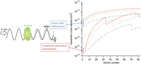
Figure 1.
(Left) Schematic diagram of how X-rays pass through object. Dashed line shows X-ray wave without object, and solid with object. (Right) Dependence of interaction cross section on atomic number for X-rays (solid, dashed, and dot-dash curves correspond to those for X-ray wavelengths of 0.2 Å, 0.6 Å, and 1.0 Å, respectively). Upper curves in graph: cross section corresponding to X-ray phase shift. Lower curves in graph: cross section corresponding to X-ray absorption.
In principle, the use of X-ray phase shifts can improve sensitivity by several orders of magnitude compared with imaging methods that use X-ray absorption. This is mainly due to the fact that the cross section of the elastic scattering of X-rays by electrons (Thomson scattering) is larger than that of photoelectric absorption. As shown in the right pad of Figure 1, the phase shift cross section is several orders of magnitude larger than the absorption cross section for a given energy, especially for light elements with small atomic numbers. By taking quantitative X-ray phase-contrast images from various directions, the so-called phase CT can be realized. In this case, what is reconstructed in the CT is a physical quantity corresponding to the deviation of the refractive index from 1 (refractive index decrement) for X-rays, which is proportional to the density of electrons per unit volume, except in special cases where the energy of X-rays used is close to an absorption edge. The refractive index decrement is about to , which is so small that X-rays are hardly refracted, but it can be detected by special methods as described below. Note that the absorption of X-rays is described by the imaginary part of the complex refractive index, which is about to several orders of magnitude smaller.
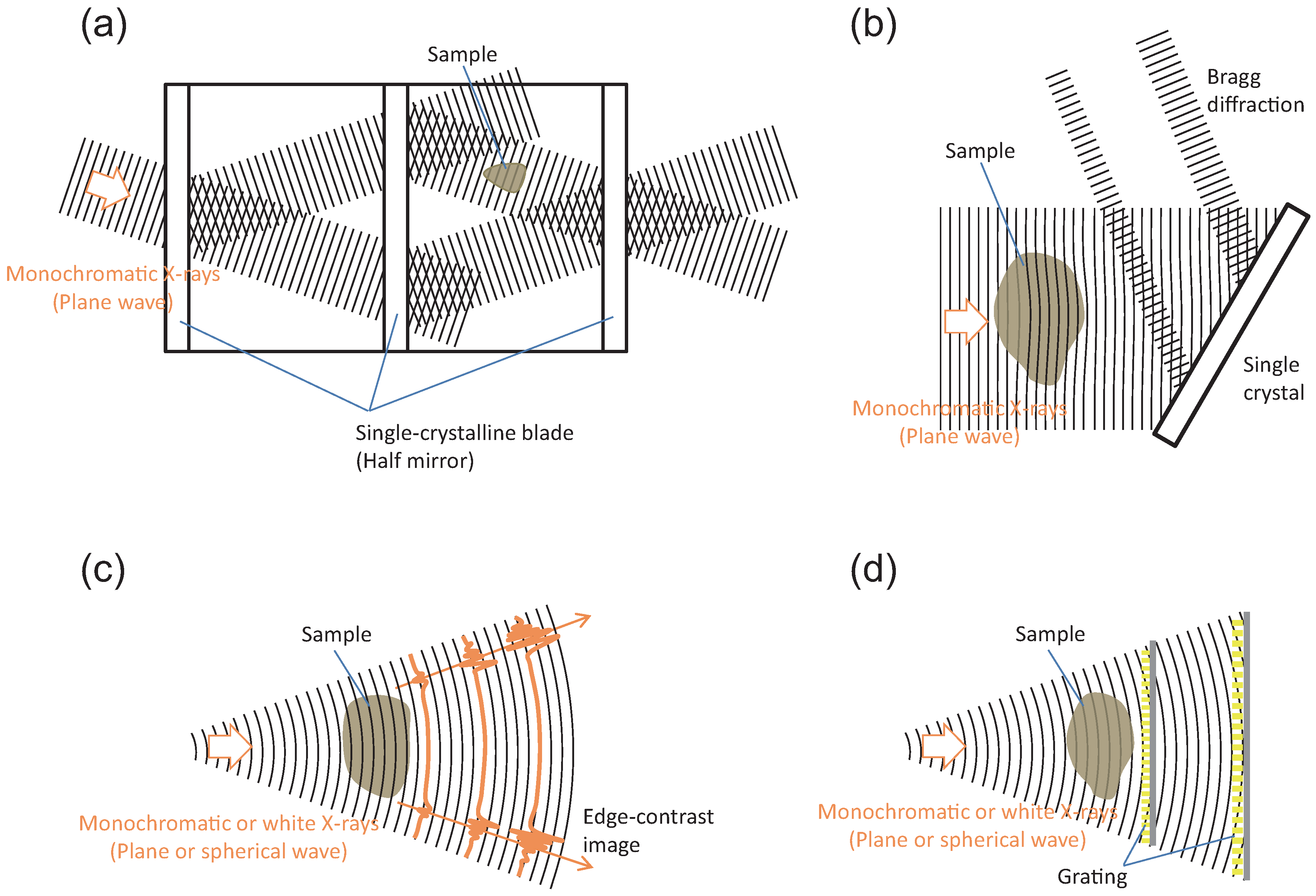
Four typical optical systems that have been proposed as methods for realizing X-ray phase-contrast imaging are compared in Figure 2. The method in Figure 2a is called “crystal interferometry” [6,7,8,9], which uses a Mach–Zehnder interferometer using Bragg reflection by a single crystal. Figure 2b shows diffraction enhanced imaging (DEI) [10,11,12], a method using an analyzer crystal, which detects the slight refraction of X-rays by an object by utilizing the very small angular width of the Bragg reflection of a single crystal (about 10 rad). The imaging methods in Figure 2a,b require monochromatic X-rays, so the measurement time for obtaining a projection image is generally on the order of seconds even when highly brilliant synchrotron radiation X-rays are used. The methods in Figure 2c,d are called the “propagation-based method” [13,14,15,16] and “grating interferometry” [17,18,19,20,21,22,23,24], respectively, and can use X-rays with a wide energy bandwidth (continuous X-rays) and spherical waves, which means that high-intensity X-rays can be used. Therefore, they are suitable for imaging with a high temporal resolution. The propagation-based method can be realized with a very simple configuration consisting only of a sample and an image detector. Images with enhanced edges can be obtained on the basis of the interference between slightly refracted X-rays inside and outside the boundaries of the structures in a sample. However, the pseudo-homogeneous assumption [16] is required for the quantitative analysis of the phase shift. Grating interferometry, in comparison, allows for quantitative imaging without any special assumptions. Another advantage of grating interferometry over the propagation-based method is its multi-modality; three independent projection images, absorption, differential-phase, and visibility-contrast images [23,24] can be obtained, as shown in Figure 3.
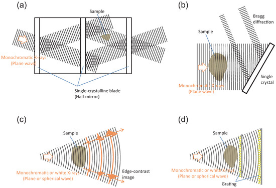
Figure 2.
Typical X-ray phase-contrast imaging techniques. (a) Crystal interferometry, (b) diffraction enhanced imaging (DEI) using analyzer crystals, (c) propagation-based method, and (d) X-ray grating interferometry.
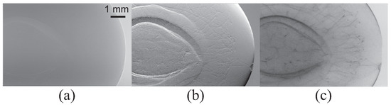
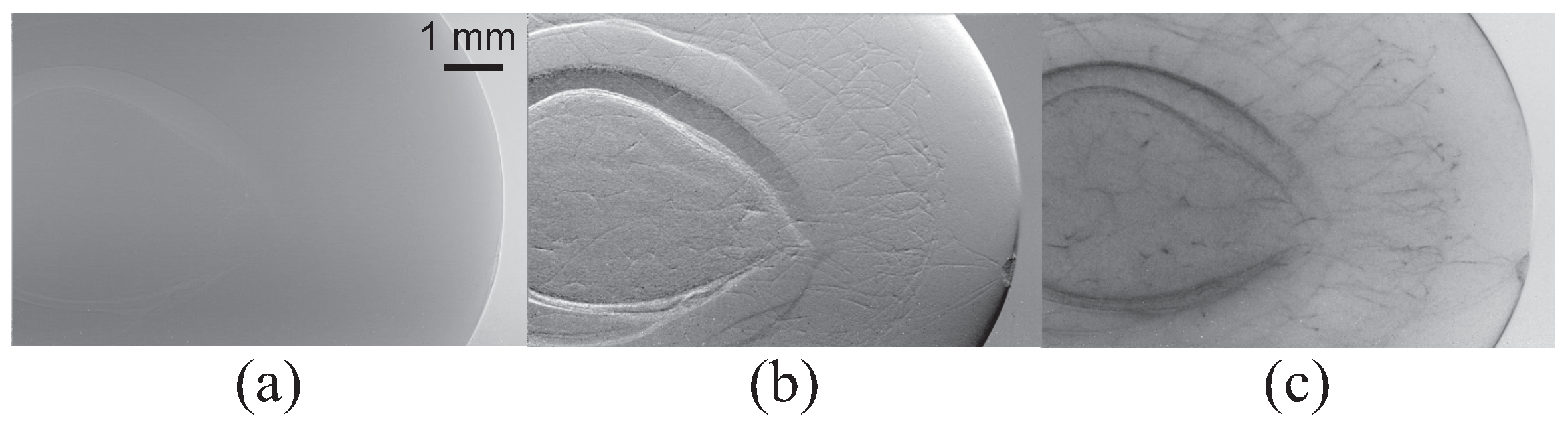
Figure 3.
Three independent projection images obtained by X-ray grating interferometry. (a) Absorption, (b) differential-phase, and (c) visibility-contrast images of cherry.
2.2. X-ray CT
Since its development in the 1970s, X-ray CT has been used in a wide range of fields including medical diagnosis and non-destructive testing. Hounsfield and Cormack were awarded the Nobel Prize in Physiology or Medicine in 1979 for their work on X-ray CT. In CT, a projection of a physical quantity is obtained experimentally in a number of directions. Here, the projection is mathematically just a line integral along a certain direction. For example, the projection of the physical quantity in the direction parallel to the y-axis is given by
Solving the inverse problem of obtaining a tomogram, , from a set of projections in many directions is called “tomographic reconstruction” [3]. We can obtain a three-dimensional image, , by stacking tomograms in the z direction.
In the case of visible light transmitted through a transparent object, the deviation in the refractive index from 1 is generally large, so it is not easy to obtain a projection experimentally. However, in the case of X-rays, the interpretation of an experimentally acquired projection image becomes much easier since X-rays are only slightly refracted by materials.
In X-ray CT using absorption, which is historically the oldest, projections of the linear absorption coefficient are obtained experimentally from X-ray transmission, and a three-dimensional image of the linear absorption coefficient is reconstructed. In the case of X-ray CT using phase shift, projections of the refractive index decrement are obtained, and a three-dimensional image of , which is approximately proportional to the number density of electrons, is reconstructed. Note that, for a synchrotron radiation beam, a tomographic reconstruction algorithm for a plane wave can be used because it can be approximated as a plane wave, while CT measurement using a laboratory X-ray source requires a tomographic reconstruction algorithm [25] for a cone beam for a large sample.
3. High-Speed X-ray CT
3.1. With Sample Rotation
The X-ray CT scanners commonly used in hospitals generally take several tens of seconds to several tens of minutes to take a 3D image. In the case of medical X-ray CT, an X-ray source and X-ray image detector are rotated around a target object in order to capture projection images from many directions. The speed of these rotations places a limit on the measurement time. Sub-second scan times have been achieved in state-of-the-art devices [26], but now, the intensity of the X-rays is an issue. A low-brilliance X-ray source based on bombarding a target material with accelerated electrons is commonly used in hospitals, and the melting of the target determines the intensity limit. Therefore, it is necessary for high-speed measurements to sacrifice the spatial resolution of the X-ray image detector to increase the number of counts for each pixel.
Time scales that can be perceived by the human eye have been the mainstream for not only X-ray CT but also other methods of non-destructive three-dimensional observation of the interior of objects opaque to visible light. Figure 4 outlines the temporal and spatial resolutions of various 3D visualization methods for samples opaque to visible light, including X-ray CT. It can be seen that the domain of millisecond- and micrometer-order spatio-temporal resolution introduced in this paper has never been explored. The pink zone in the figure shows, as an example, the spatial and temporal resolutions suitable for observing the movement of animals. This zone roughly represents kinetic speed determined by metabolic rate × biological time. The zone corresponding to the mechanical motion of artifacts (green zone) is one or two orders of magnitude higher than this. Many of the phenomena we come across in our daily lives occur in these zones, making them extremely important subjects of research in science, technology, and industry. Various applications are possible for measurement methods that can access these temporal and spatial scales, from academic research, such as observing phenomena inside living animals (e.g., insects), the failure process of materials, and the behavior of liquids, to industrial applications, such as developing intelligent materials, and dynamic biomimetics applications.
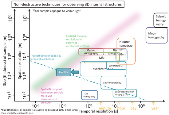
Figure 4.
Non-destructive techniques for observing 3D internal structures of samples opaque to visible light.
The trade-off between temporal and spatial resolutions (dashed line) is also shown in Figure 4. To increase the temporal resolution, it is generally sufficient to sacrifice the spatial resolution. In fact, temporal resolution on the order of milliseconds has been achieved for a spatial resolution reduced to the order of millimeters. It is worth noting, however, that the direction of this trade-off relationship is close to orthogonal to the pink and green zones. In other words, the smaller the observation object, the larger the demand for high-speed viewing, but improving both spatial and temporal resolutions is often technically challenging.
Thus, how can we realize high-speed X-ray CT that far exceeds the limits of what the human eye can perceive? It is impossible to rotate the X-ray source and the X-ray image detector of a hospital X-ray CT scanner at the speed that is needed. Additionally, the intensity of X-ray sources used at the laboratory level is insufficient.
Highly intense synchrotron radiation X-rays can solve this problem [27,28,29,30,31]. The authors succeeded in X-ray CT with an imaging time on the order of milliseconds by using a third-generation synchrotron radiation source and rotating samples at high speed [27,28,29]. The experiments were performed at the experimental station BL28B2 at SPring-8, a large synchrotron radiation facility. Third-generation synchrotron radiation sources such as SPring-8 are capable of producing much more brilliant X-rays (i.e., a high-intensity X-ray beam from a small light source) than laboratory X-ray sources. The small size of the light source allows us to use high-spatial-coherence X-rays, which is suitable for X-ray phase-contrast imaging. The advantage of this imaging is that it is more sensitive than X-ray absorption imaging as described in Section 2.1. With this imaging, the experimentally obtained refractive index decrement for X-rays is taken as the physical quantity in Equation (1).
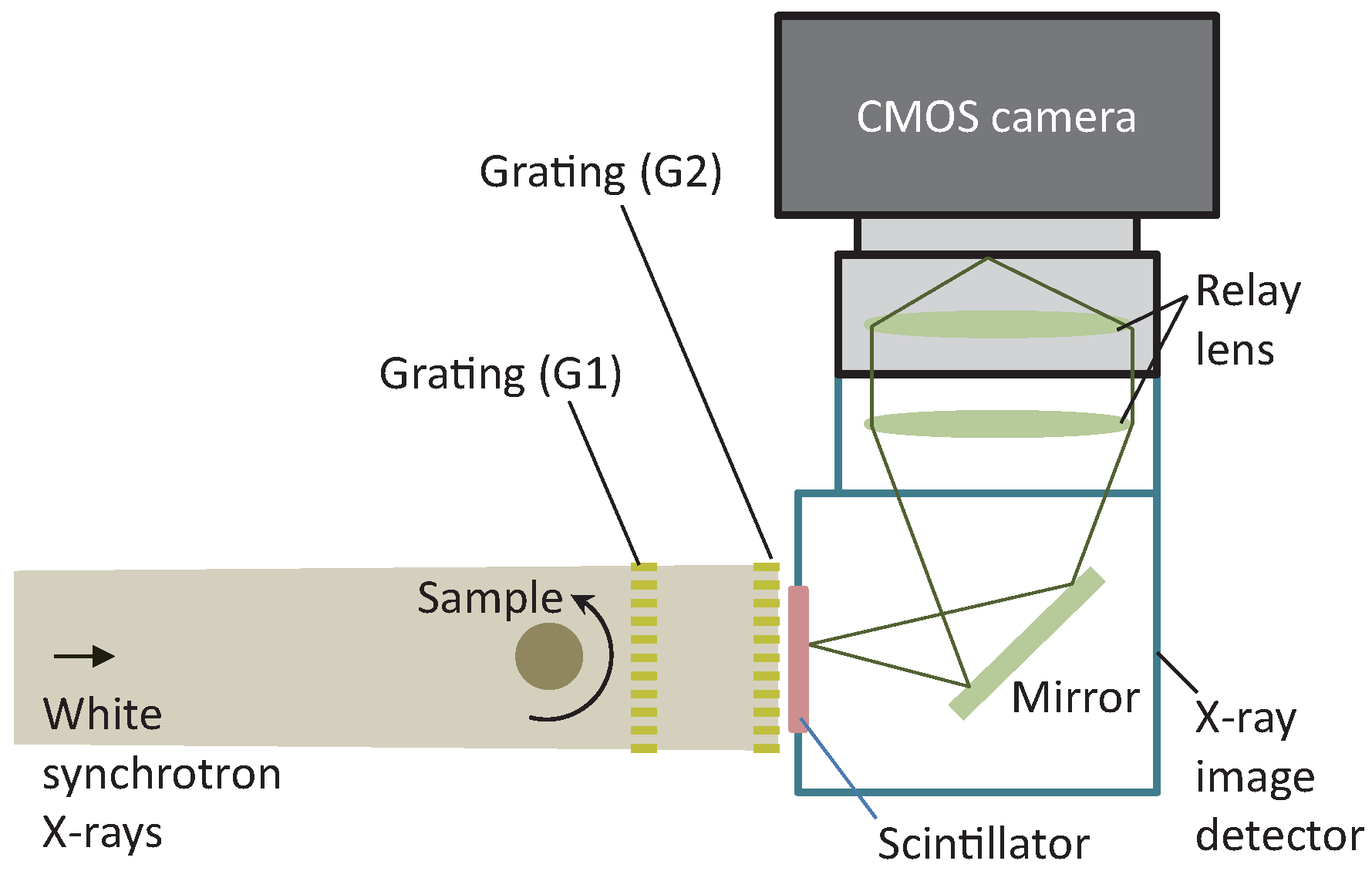
The experimental setup (side view) is shown in Figure 5. Here, we used X-ray grating interferometry. As described in Section 2.1, this method uses gratings for X-rays (the two gratings in Figure 5), and it has the advantage that a white synchrotron radiation beam with high intensity and a relatively large area can be used.
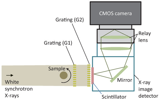
Figure 5.
Experimental setup (side view) of millisecond X-ray CT conducted by X-ray grating interferometry using white synchrotron radiation at BL28B2 of SPring-8 [27,28,29]. Copyright (2017, 2018) The Japan Society of Applied Physics.
In grating interferometry [32], a self-imaging phenomenon called the Talbot effect [33,34] is used. The Talbot effect occurs when a periodic object such as a grating is illuminated by light with a spatial coherence length comparable to or larger than the period of the object. The self-images generated downstream of the object are deformed when light is refracted by a sample located in front of or behind the object. From this deformation, we can obtain an image of the change in the propagation direction due to the refraction by the sample, which corresponds to the differential phase image for the sample.
For the X-ray grating interferometer shown in Figure 5, we used a -phase grating (G1) designed for an X-ray energy of 25 keV, whose lines are aligned in the horizontal direction. The grating was located at a distance of 44 m from the X-ray source with a full width at half maximum (FWHM) of 28.7 m, which, from the van-Cittert Zernike theorem [35], provides a spatial coherence length at G1 sufficiently larger than the period of G1 (5.3 m). Another 5.3 m-period grating (a 60 m-thick gold absorption grating (G2) was located on a self-image generated at a distance of 283 mm downstream of G1 to detect the deformation of the self-image as moiré fringes. Both gratings were made of gold on 200 m-thick Si substrates.
To achieve high-speed imaging, an indirect imaging-type X-ray detector was used that consists of a scintillator, a lens coupling system, and a high-speed camera. A scintillator is a material that converts X-rays into visible light [36]. The 40 m-thick single-crystal Ce:GAGG scintillator used in this experiment had a very short luminescence decay time of 53 ns and a large luminescence intensity [37]. As a high-speed camera, we used a CMOS camera (Photron FASTCAM Mini AX100), which is capable of capturing 1024 × 1024 full-frame images at a maximum of 4000 frames per second. The effective pixel size at the sample position was 9.9 m, and the spatial resolution was 21 m.
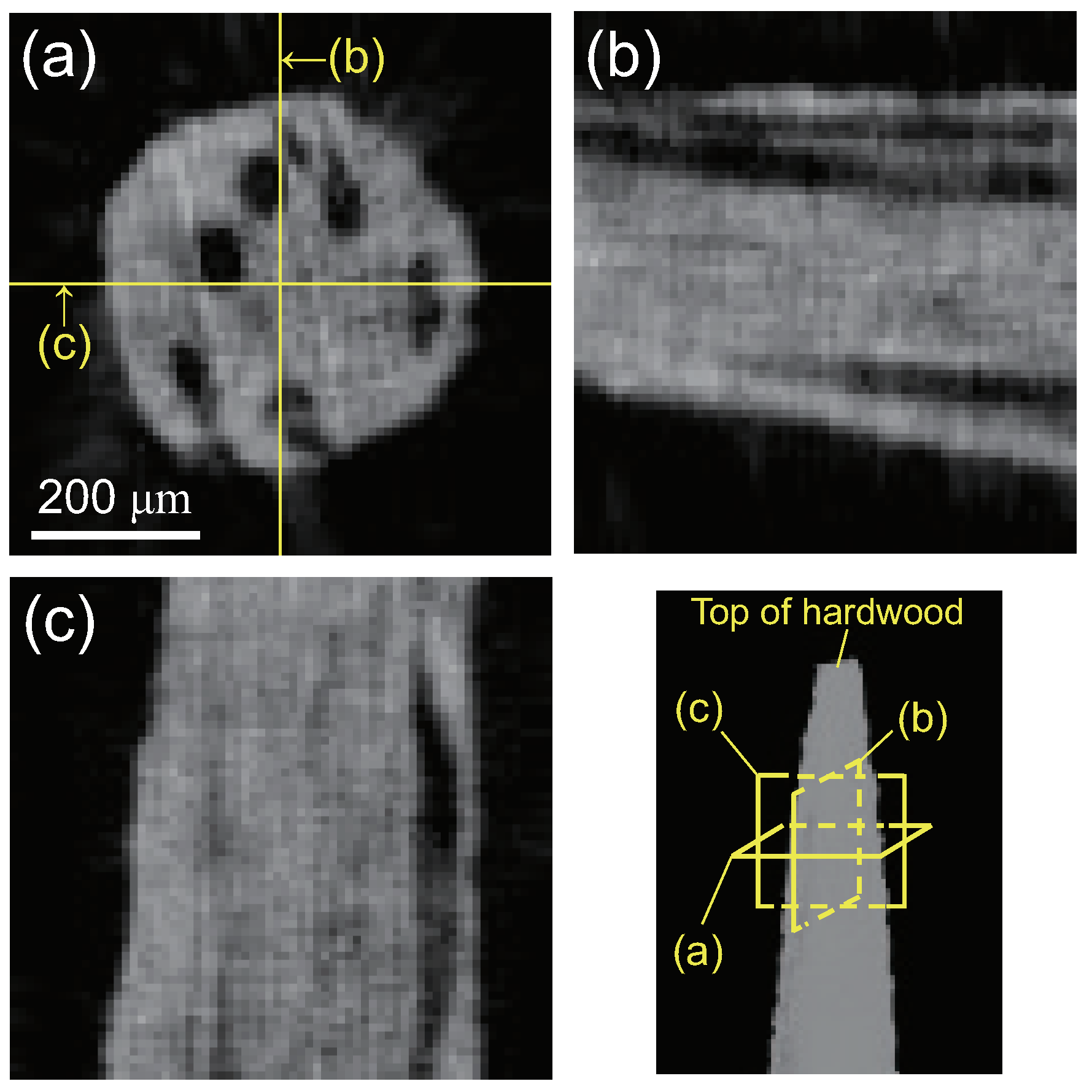
Figure 6 shows a 3D phase tomogram of a toothpick (piece of hardwood) as an example (3D CT reconstruction image of the refractive index decrement ) [29]. This 3D image was obtained on the basis of a fringe scanning method [38,39,40]: a three-step equal-sampling fringe scanning was performed by continuously moving G2 and rotating the sample. The speed of G2 was tuned so that it was moved by one period in the vertical direction while the sample was rotated through three turns. Since three projection images in the same projection angle are necessary for the three-step fringe scanning, 2.5 turns of the sample are required for CT reconstruction for the synchrotron beam. The sample was rotated at 33,850 rpm, so that the 3D image was captured in 4.43 ms. The projection images were captured at a frame rate of 127,500 frames per second (7.8 s per frame), and the 3D phase tomogram was obtained from 113 differential phase images by the filtered back-projection algorithm. Note that, for the projection images, the field of view was reduced to be 128 × 64 pixels at the frame rate because there is generally a trade-off between the frame rate and the field of view of a high speed camera. The specimen was not stained with a contrast agent, but high contrast images of the internal structure, such as canals and xylem fibers, were obtained by using the phase of the X-rays, even though the material is composed of light elements that absorb X-rays very little.
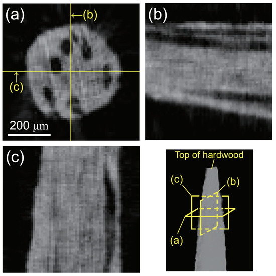
Figure 6.
Phase tomogram of piece of hardwood obtained by X-ray grating interferometry using white synchrotron radiation (exposure time: 4.43 ms) [29]. Copyright (2018) The Japan Society of Applied Physics (a) Axial, (b) sagittal, and (c) coronal images.
Recently, dynamic 4D observation has also become possible. Figure 7 demonstrates 4D X-ray CT with a temporal resolution of 10 ms for the process of breaking rubber while pulling it [41,42]. The upper left pad of Figure 7 shows a schematic illustration of the rotating device for the 4D X-ray CT. It comprises two coaxial inverter-driven motors, which can be electrically synchronized by a motor controller. The motors for rotation are mounted on two carriages on parallel stainless-steel rails and are uniaxially movable along the rails in the direction parallel to the rotation axis (in the horizontal direction). The rubber sample was bonded on top of the motor axes, as shown in the upper right pad of Figure 7, and stretched while rotating at high speed.
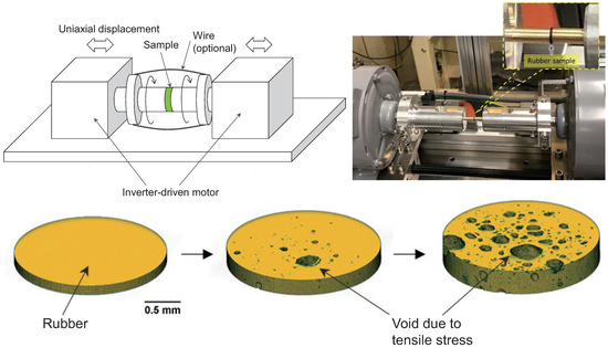
Figure 7.
Real-time 4D observation of rubber tensile fracture process (10-ms temporal resolution) [41,42]. Upper: rotation device for high-speed X-ray CT, lower: 4D tomograms of tensile fracture process of rubber.
The indirect imaging-type X-ray detector with a 10 m-thick single crystal Ce:GAGG scintillator was employed for the 4D X-ray CT. Here, a CMOS camera with a higher frame rate (FASTCAM Nova S12 from Photron, 1024 × 1024 full frame at a maximum of 12,800 frames per second) was used for a high-speed camera.
The sample was located at a distance of 4.7 m upstream of the detector, and full-frame projection images (propagation-based phase-contrast images) were obtained at a frame rate of 12,800 frames per second. The sample was rotated at 3000 rpm, so that the number of projections for half turn of the sample was 128. The effective pixel size was 4.5 m at the sample position, which corresponds to the spatial resolution of the projection images. It was confirmed from the projection images, that the sample was stretched at a constant rate of 1226.8 m/s.
The lower pad of Figure 7 demonstrates a series of the reconstructed 3D images, which is the world’s fastest example of active observation of a micron-scale fracture process using X-ray CT, and it clearly shows the formation of voids inside the rubber. Note that this example is an absorption tomogram, but since the X-rays transmitted through the sample interfered with each other to produce an edge-enhanced projection image, the tomogram also has an enhanced boundary.
3.2. With Compressed Sensing
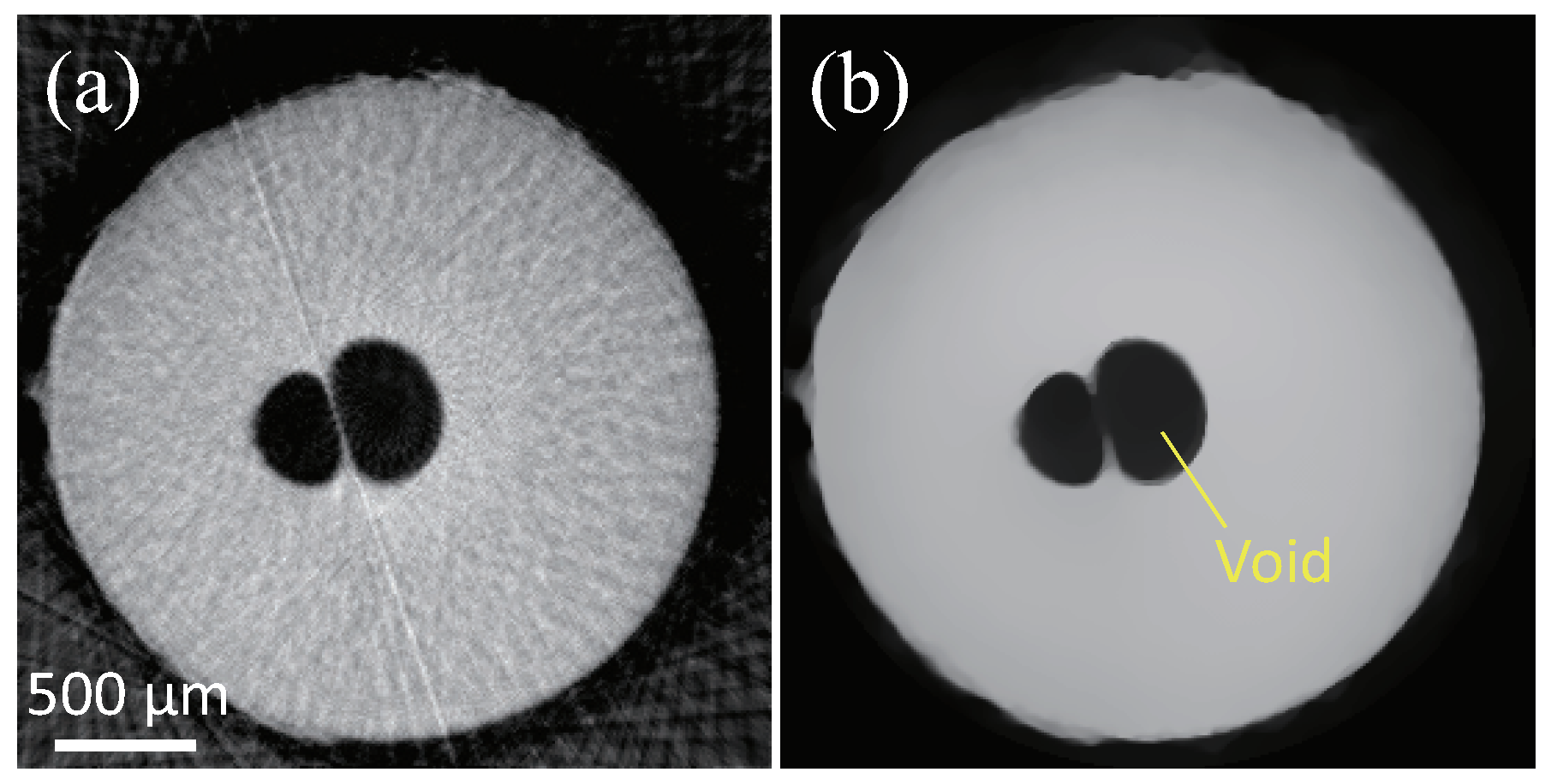
If we try to further shorten the acquisition time, the number of projections has to be reduced because the frame rate cannot be increased while maintaining the field of view. Figure 8a shows a tomogram of a polypropylene (PP) sphere with a diameter of 3/32 inches acquired at 2.0 ms. Here, the projection images were obtained by the same experimental setup as that of Figure 5, but the Fourier transform method [43] was used instead of the fringe scanning method. In the Fourier transform method, a differential phase image can be obtained from a projection image with fine moiré fringes, so that higher temporal resolution is realized than that of the fringe scaning method, although the spatial resolution becomes worse up to the period of the moiré fringes. We obtained the projection images at a frame rate of 37,500 frames per second with a field of view of 256 × 256 and rotated the sample at a speed of 29,605 rpm. To increase the field of view, the so-called offset CT was used: the two projections from opposite directions were combined to obtain a single projection image. Since only 76 projections for a half turn of the sample can be obtained, using the classical CT reconstruction algorithm (filtered back-projection algorithm) results in radial artifacts as shown in the left pad in the figure.
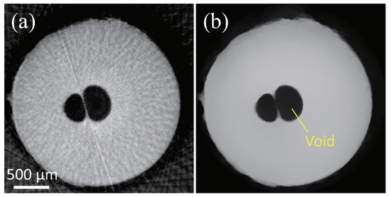
Figure 8.
Phase tomogram of polypropylene (PP) sphere taken with measurement time of 2.0 ms [28].Copyright (2017) The Japan Society of Applied Physics (a) Reconstruction result using conventional filtered back-projection algorithm. (b) Reconstruction result using TV norm.
A compressed sensing-based CT reconstruction method has recently attracted attention as a solution to this problem [28,44,45,46,47,48,49]. In this method, images are recovered from a small number of observation data samples by using the inherent sparsity of images. Sparsity is often inherent in images obtained from the natural world. For example, if we carry out a wavelet transform of an image, extract only 10% of its components, and carry out an inverse transform, the resulting image will be almost indistinguishable from the original. In other words, even if the number of data samples is insufficient, the original image can be obtained by applying an appropriate linear transformation (called sparsify transformation) since the number of non-zero components to be recovered can be approximated to a small number.
The problem of compressed sensing can be mathematically generalized as follows. Suppose that an original physical quantity, , results in the observed data (), as expressed in the following equation.
where the inner product with expresses the ith sampling. Additionally, suppose that the original physical quantity can be expanded by the basis () of the sparsify transformation as follows
Substituting Equation (3) into Equation (2) and defining , we obtain
that is, the vector with components can be expressed by the product of the matrix and the vector with components of and , respectively. If , we can find by calculating the inverse; if and there is no satisfying , we can find the least-squares solution (the solution that minimizes () by using the so-called Moore–Penrose pseudo-inverse matrix, for example. If , the solution is indefinite and becomes an ill-posed problem. However, if the number K of non-zero components of is small and , then there is a possibility of finding the K non-zero components. The goal of compressed sensing is to solve the problem of recovering the sparse vector from under the constraint of . The problem can be formulated as
where the -norm of is defined by
That is, in Equation (5) is called the -norm, which is defined as the number of non-zero components of vector . If we know where the non-zero components are, we can find by extracting only the non-zero components and calculating the inverse matrix, but the difficulty of the problem lies in the fact that we do not know where the non-zero components are.
The problem setup in Equation (5) can be applied to X-ray CT. In this case, the vector of all the pixel values of the projection images acquired from various projection directions corresponds to the observed data , corresponds to a tomogram, and the transformation coefficients with the sparsify transformation correspond to . In the case where the observed data contains random errors, the constraint in Equation (5) can be included as a penalty term, resulting in the following optimization problem.
where is the square root of the sum of the squared components of the vector (i.e., the distance in Euclidean space), called the “ norm.” The hyperparameter (>0) regulates the degree of sparsity; the larger , the stronger the degree of sparsity, and the closer the solution to that of Equation (5). The -norm optimization problem in Equation (7) is known to be an NP-hard problem when M, N, and K are large, and it can be solved numerically by replacing it with the -norm optimization problem as follows.
where the -norm is the sum of the absolute values of each component of the vector . Equation (8) can be interpreted as a formulation of the problem of finding the that minimizes under the constraint that is constant, using Lagrange’s undecided multiplier . Using the norm instead of the norm makes it easier to choose a sparse solution. The reason can be intuitively explained as shown in Figure 9. We consider a two-dimensional vector (i.e., ) for simplicity. In the figure, a line with constant and a contour line of are drawn. It can be seen that the solution that minimizes under the constraint of constant is on a coordinate axis in the figure, which is a sparse solution (the solution with ). Note that the optimization problem in Equation (7) is equivalent to the so-called sparse modeling, i.e., the method of estimating unknown parameters by adding a penalty term to estimate an original physical quantity under the assumption that the parameters are sparse. For image data such as CT image reconstruction, the total variation (TV) norm is often used as it has essentially the same effect as taking the norm after the sparsify transformation. The TV norm of image , , is defined by the following equation:
Here, and are the differences in pixel values between the kth pixel and its neighbors in the horizontal and vertical directions, respectively. This problem can be formulated as
where is an operator representing the projection operation. Using the TV norm, we can obtain an image with a sparse number of edges (i.e., an image in which the edges are strongly preserved and the pixel values within the region surrounded by the edges are almost uniform).
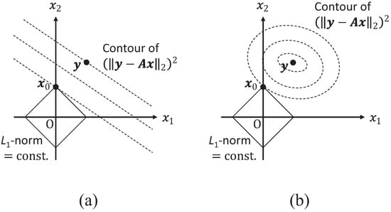
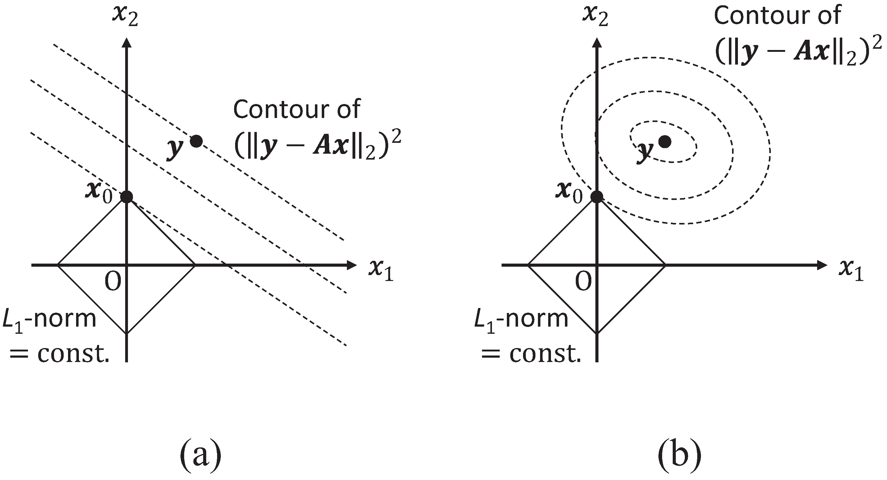
Figure 9.
Schematic illustration of how sparse solutions are more easily selected by using norm for ((a) , (b) ). Solid line represents line with constant norm, and dashed line represents contour line of . In figure, is point that minimizes under constraint of constant norm, i.e., solution to optimization problem in Equation (7) (solution with ). Note that cases of can be illustrated similarly to (b), but is generally not in - plane.
Figure 8b shows the result of using one of the CT reconstruction algorithms based on such compressed sensing, and it can be seen that the image is free of the artifacts seen in the left panel.
3.3. Without Sample Rotation
The tomogram in Figure 7 was obtained by pulling the sample while rotating it at a high speed of 3000 rpm (50 Hz). To further increase the temporal resolution, the sample needs to be rotated at an even higher speed. However, when the rotation speed was increased by several times, the sample was deformed by centrifugal force, so no CT reconstruction image could be obtained. Rotating the specimen at high speed not only causes the centrifugal force to be large but also imposes various restrictions on such experiments, such as difficulty in controlling the environment of the specimen and inapplicability to fluid specimens. Therefore, the authors aimed to develop a method for realizing synchrotron radiation X-ray CT without the need to rotate samples.
Since it is not possible to rotate the synchrotron radiation source around a sample, the authors developed a multi-beam optical system for millisecond X-ray CT without sample rotation. There are three ways to change the propagation direction of X-rays: reflection, refraction, and diffraction, but the change in propagation direction that can be achieved by the first two methods is on the order of mrad. The authors selected diffraction (Bragg reflection at a single crystal with high perfection), which can change the propagation direction most significantly, due to the need to cover a wide angular range of projection directions in X-ray CT.
However, the resonance width of highly perfect Bragg reflection is very narrow (about 10 rad in terms of the angle of incidence) due to the dynamical diffraction effect of X-rays, which generally requires a very expensive, precise optical system. Therefore, the authors used white synchrotron radiation and aimed to precisely control multiple reflected beams at the same time by precisely curving a thin single-crystal wafer.
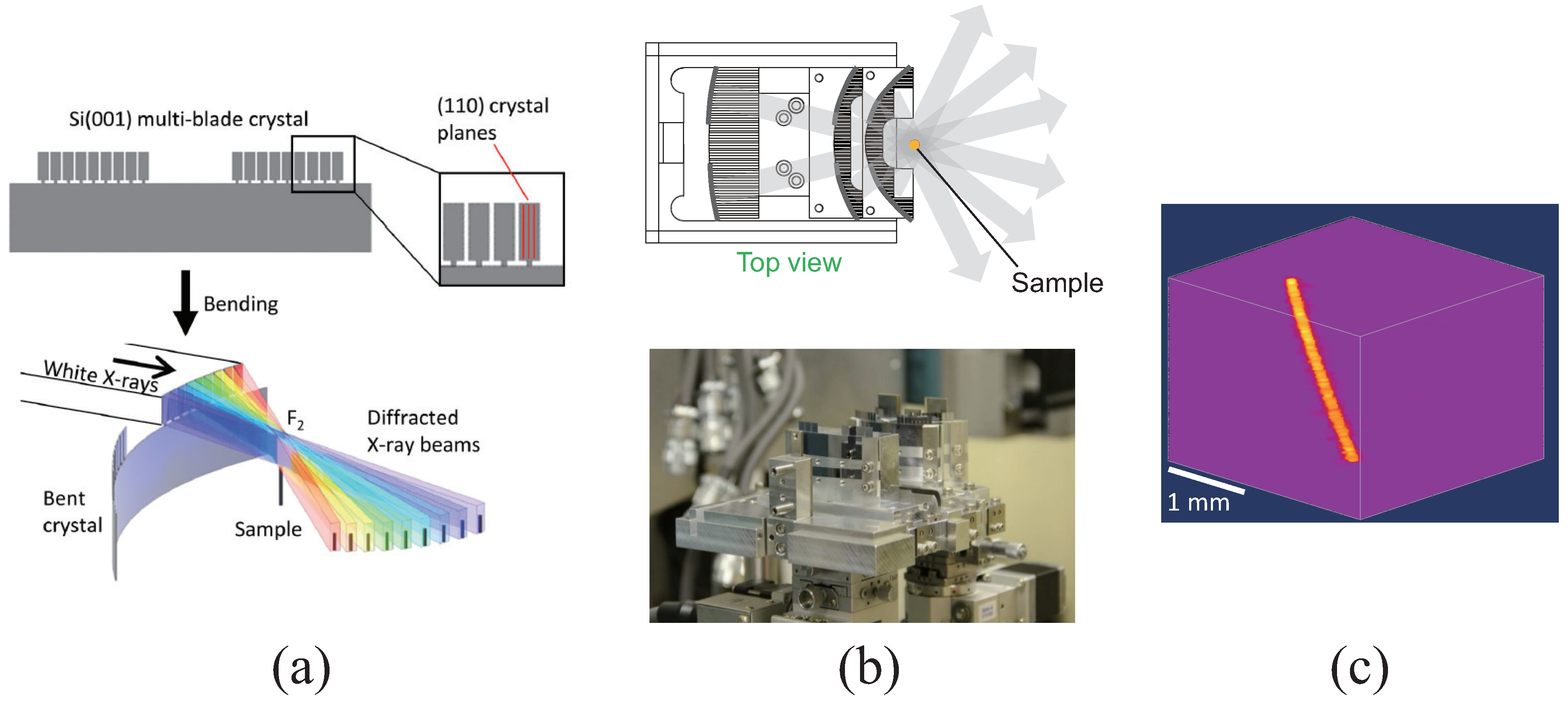
Figure 10a shows the principle of the multi-beaming technique we developed to realize X-ray CT without sample rotation. A 100 m-thick Si single crystal was etched into the shape shown in the upper figure of Figure 10a by microfabrication [50], and when it is bent, the small rectangular plates at the top (hereinafter called “blades”) point in different directions in accordance with the orientation of the lower part of the crystal. If the Si wafer is curved along a hyperbola, the reflected beams will converge toward the sample. As mentioned above, the resonance width of Bragg reflection is very narrow, so the energy bandwidth of the reflected X-rays is very small. Therefore, the transmitted X-rays can be reused. Figure 10b shows the hyperbolic-shape multi-beam optical element we developed [31]. The element can generate 32 beams covering a range of . Figure 10c is a 3D CT reconstruction image acquired with an exposure time of 1 ms using a 50-m diameter tungsten wire as a sample. The spatial resolution of the tomogram was 65 m. We used the state-of-the-art CT reconstruction algorithm based on compressed sensing described in Section 3.2.
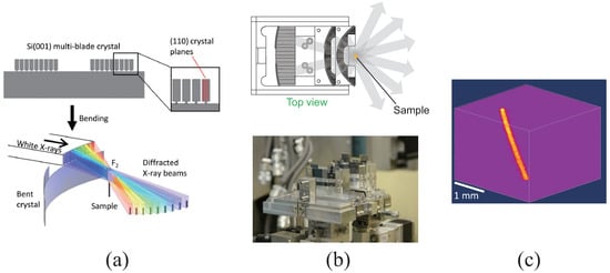
Figure 10.
(a) Multi-beam Si single-crystal optical element for millisecond time-resolution X-ray CT, (b) hyperbolic-shape multi-beam optical element covering projection directions of more than [(top) top view, (bottom) photo], and (c) three-dimensional reconstructed image of tungsten wire with diameter of 50 m acquired by synchrotron radiation multi-beam optics at 1 ms [31].
4. Summary
In this paper, we introduced synchrotron radiation X-ray CT with a millisecond temporal resolution, which is far beyond the limit of what can be perceived by the human eye. Temporal resolutions of 2 to 10 ms have been achieved with sample rotation and of 1 ms without sample rotation (with synchrotron radiation multi-beam optics). The spatio-temporal resolutions we achieved recently are summarized in Figure 11, in comparison with those of other representative reports [30,51,52,53,54,55,56,57,58]. The multi-beam optics, together with the multi-beam X-ray image detector [59,60] developed by the authors, enables 4D observation of fluid samples and living animals on the millisecond order, and since various sample environments can be introduced, it is expected to have a ripple effect in a wide range of fields from basic research in materials and life sciences to industrial applications. Its potential applications include observing fracture processes of polymer materials and adhesive interfaces and dynamic biomimetics research conducted on the basis of the 4D observation of live insects. Our techniques can be used to explore the frontiers of the 4D spatio-temporal domain of m and ms orders and is expected to unveil mechanisms of various non-repeatable and non-equilibrium phenomena that have never been uncovered by other techniques.
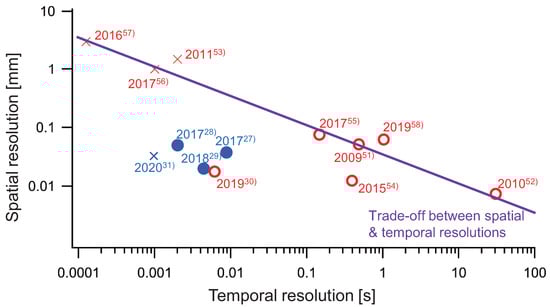
Figure 11.
Summary of spatio-temporal resolutions we achieved (blue filled circles and cross) in comparison with those of other representative reports (red open circles and crosses). Circles and crosses represent achievements with and without sample rotation, respectively.
Funding
This research was funded by JST CREST (Grant No. JPMJCR1765), JSPS Grants-in-Aid for Scientific Research (Grant No. JP15H03590, JP26600137), and Sumitomo Rubber Industries, Ltd. Hyogo, Japan.
Institutional Review Board Statement
Not applicable.
Informed Consent Statement
Not applicable.
Acknowledgments
The experiments using synchrotron radiation were conducted under the general proposal (2016A–2019B) and the long-term use proposal (2020A0176) of SPring-8, whose preliminary experiments were also performed at SAGA-LS (1909080S).
Conflicts of Interest
The authors declare no conflict of interest.
References
- Fossum, E.R.; Hodongwa, D.B. A review of the pinned photodiode for CCD and CMOS image sensors. IEEE J. Electron Devices Soc. 2014, 2, 33–43. [Google Scholar] [CrossRef]
- Kuroda, R.; Suzuki, M.; Sugawa, S. Over 100 million frames per second high speed global shutter CMOS image sensor. Proc. SPIE 2019, 11051, 1105157. [Google Scholar]
- Als-Nielsen, J.; McMorrow, D. Elements of Modern X-ray Physics, 2nd ed.; Wiley: Chichester, UK, 2011. [Google Scholar]
- Fitzgerald, R. Phase-sensitive x-ray imaging. Phys. Today 2000, 53, 23–26. [Google Scholar] [CrossRef]
- Nugent, K.A. Coherent methods in the X-ray sciences. Adv. Phys. 2010, 59, 1–99. [Google Scholar] [CrossRef] [Green Version]
- Bonse, U.; Hart, M. An X-ray interferometer. Appl. Phys. Lett. 1965, 6, 155–156. [Google Scholar] [CrossRef]
- Momose, A.; Takeda, T.; Itai, Y.; Hirano, K. Phase-contrast X-ray computed tomography for observing biological soft tissues. Nat. Med. 1996, 2, 473–475. [Google Scholar] [CrossRef]
- Takeda, T.; Yoneyama, A.; Wu, J.; Thet-Thet-Lwin; Momose, A.; Hyodo, K. In vivo physiological saline-infused hepatic vessel imaging using a two-crystal-interferometer-based phase-contrast X-ray technique. J. Synchrotron Rad. 2012, 19, 252–256. [Google Scholar] [CrossRef]
- Yoneyama, A.; Nambu, A.; Ueda, K.; Yamada, S.; Takeya, S.; Hyodo, K.; Takeda, T. Phase-contrast X-ray imaging system with sub mg/cm3 density resolution. J. Phys. Conf. Ser. 2013, 425, 192007. [Google Scholar] [CrossRef]
- Davis, J.; Gao, D.; Gureyev, T.E.; Stevenson, A.W.; Wilkins, S.W. Phase-contrast imaging of weakly absorbing materials using hard X-rays. Nature 1995, 373, 595–598. [Google Scholar] [CrossRef]
- Chapman, D.; Thomlinson, W.; Johnston, R.E.; Washburn, D.; Pisano, E.; Gmúr, N.; Zhong, Z.; Menk, R.; Arfelli, F.; Sayers, D. Diffraction enhanced x-ray imaging. Phys. Med. Biol 1997, 42, 2015–2025. [Google Scholar] [CrossRef] [Green Version]
- Ando, A.; Sugiyama, H.; Maksimenko, A.; Pattanasiriwisawa, W.; Hyodo, K.; Xiaowei, Z. A new optics for dark-field imaging in X-ray region ‘Owl’. Jpn. J. Appl. Phys. 2001, 40, L844–L846. [Google Scholar] [CrossRef]
- Snigirev, A.; Snigireva, I.; Kohn, V.; Kuznetsov, S.; Schelokov, I. On the possibilities of x-ray phase contrast microimaging by coherent high-energy synchrotron radiation. Rev. Sci. Instrum. 1995, 66, 5486–5492. [Google Scholar] [CrossRef]
- Wilkins, S.W.; Gureyev, T.E.; Gao, D.; Pogany, A.; Stevenson, A.W. Phase-contrast imaging using polychromatic hard X-rays. Nature 1996, 384, 335–338. [Google Scholar] [CrossRef]
- Cloetens, P.; Barrett, R.; Baruchel, J.; Guigay, J.-P.; Schlenker, M. Phase objects in synchrotron radiation hard x-ray imaging. J. Phys. D 1996, 29, 133–146. [Google Scholar] [CrossRef]
- Paganin, D.; Mayo, S.C.; Gureyev, T.E.; Miller, P.R.; Wilkins, S.W. Simultaneous phase and amplitude extraction from a single defocused image of a homogeneous object. J. Microsc. 2002, 206, 33–40. [Google Scholar] [CrossRef]
- David, C.; Nóhammer, B.; Solak, H.H. Differential x-ray phase contrast imaging using a shearing interferometer. Appl. Phys. Lett. 2002, 81, 3287–3289. [Google Scholar] [CrossRef]
- Momose, A.; Kawamoto, S.; Koyama, I.; Hamaishi, Y.; Takai, K.; Suzuki, Y. Demonstration of x-ray Talbot interferometry. Jpn. J. Appl. Phys. 2003, 42, L866–L868. [Google Scholar] [CrossRef]
- Weitkamp, T.; Diaz, A.; David, C.; Pfeiffer, F.; Stampanoni, M.; Cloetens, P.; Ziegler, E. X-ray phase imaging with a grating interferometer. Opt. Express 2005, 13, 6296–6304. [Google Scholar] [CrossRef]
- Momose, A.; Yashiro, W.; Takeda, Y.; Suzuki, Y.; Hattori, T. Phase tomography by x-ray Talbot interferometry for biological imaging. Jpn. J. Appl. Phys. 2006, 45, 5254–5262. [Google Scholar] [CrossRef]
- Pfeiffer, F.; Weitkamp, T.; Bunk, O.; David, C. Phase retrieval and differential phase-contrast imaging with low-brilliance X-ray sources. Nat. Phys. 2006, 2, 258–261. [Google Scholar] [CrossRef]
- Yashiro, W.; Takeda, Y.; Momose, A. Efficiency of capturing a phase image using cone-beam x-ray Talbot interferometry. J. Opt. Soc. Am. A 2008, 25, 2025–2039. [Google Scholar] [CrossRef]
- Pfeiffer, F.; Weitkamp, T.; Bunk, O.; David, C. Hard-X-ray dark-field imaging using a grating interferometer. Nat. Mater. 2008, 7, 134–137. [Google Scholar] [CrossRef]
- Yashiro, W.; Terui, Y.; Kawabata, K.; Momose, A. On the origin of visibility contrast in x-ray Talbot interferometry. Opt. Express 2010, 18, 16890–16901. [Google Scholar] [CrossRef]
- Feldkamp, L.A.; Davis, L.C.; Kress, J.W. Practical cone-beam algorithm. J. Opt. Soc. Am. A 1984, 1, 612–619. [Google Scholar] [CrossRef] [Green Version]
- Inoue, Y.; Matsuoka, Y.; Kobayashi, S.; Hishida, N.; Yamashita, Y.; Sakai, T.; Yamanaka, S.; Imanishi, T.; Ishiyama, T. “Subrina” x-ray CT scanner, sub-second scanning type. Shimadzu Rev. 2000, 57, 225–231. [Google Scholar]
- Yashiro, W.; Noda, D.; Kajiwara, K. Sub-10-ms X-ray tomography using a grating interferometer. Appl. Phys. Express 2017, 10, 052501. [Google Scholar] [CrossRef] [Green Version]
- Yashiro, W.; Ueda, R.; Kajiwara, K.; Noda, D.; Kudo, H. Millisecond-order X-ray phase tomography with compressed sensing. Jpn. J. Appl. Phys. 2017, 56, 112503. [Google Scholar] [CrossRef]
- Yashiro, W.; Kamezawa, C.; Noda, D.; Kajiwara, K. Millisecond-order X-ray phase tomography with a fringe-scanning method. Appl. Phys. Express 2018, 11, 122501. [Google Scholar] [CrossRef]
- García-Moreno, F.; Kamm, P.H.; Neu, T.R.; Búlk, F.; Mokso, R.; Schlepútz, C.M.; Stampanoni, M.; Banhart, J. Using X-ray tomoscopy to explore the dynamics of foaming metal. Nat. Commun. 2019, 10, 3762. [Google Scholar] [CrossRef]
- Voegeli, W.; Kajiwara, K.; Kudo, H.; Shirasawa, T.; Liang, X.; Yashiro, W. Multibeam X-ray optical system for high-speed tomography. Optica 2020, 7, 514–517. [Google Scholar] [CrossRef]
- Yokozeki, S.; Suzuki, T. Shearing Interferometer Using the Grating as the Beam Splitter. Appl. Opt. 1971, 10, 1575–1580. [Google Scholar] [CrossRef]
- Talbot, H.F. Facts relating to optical science. Philos. Mag. 1836, 9, 401–407. [Google Scholar]
- Patorski, K. The self-imaging phenomenon and its applications. Prog. Opt. 1989, 27, 1–108. [Google Scholar]
- Born, M.; Wolf, E. Principles of Optics, 7th ed.; Cambridge U. Press: Cambridge, UK, 1999. [Google Scholar]
- Yoneyama, A.; Baba, R.; Kawamoto, R. Quantitative analysis of the physical properties of CsI, GAGG, LuAG, CWO, YAG, BGO, and GOS scintillators using 10-, 20- and 34-keV monochromated synchrotron radiation. Opt. Mater. Express 2021, 11, 398–411. [Google Scholar] [CrossRef]
- Kamada, K.; Endo, T.; Tsutumi, K.; Yanagida, T.; Fujimoto, Y.; Fukabori, A.; Yoshikawa, A.; Pejchal, J.; Nikl, M. Composition engineering in cerium-doped (Lu,Gd)3(Ga,Al)5O12 single-crystal scintillators. Cryst. Growth Des. 2011, 11, 4484–4490. [Google Scholar] [CrossRef]
- Bruning, J.H.; Herriott, D.R.; Gallagher, J.E.; Rosenfeld, D.P.; White, A.D.; Brangaccio, D.J. Digital wavefront measuring interferometer for testing optical surfaces and lenses. Appl. Opt. 1974, 13, 2693–2703. [Google Scholar] [CrossRef]
- Schreiber, H.; Bruning, J.H. Optical Shop Testing, 3rd ed.; Malacara, D., Ed.; Wiley: Hoboken, NJ, USA, 2007; Chapter 14. [Google Scholar]
- Hack, E.; Burke, J. Invited review article: Measurement uncertainty of linear phase-stepping algorithms. Rev. Sci. Instrum. 2011, 82, 061101. [Google Scholar] [CrossRef]
- Mashita, R.; Yashiro, W.; Kaneko, D.; Bito, Y.; Kishimoto, H. High-speed rotating device for X-ray tomography with 10 ms temporal resolution. J. Synchrotron Rad. 2021, 28, 322–326. [Google Scholar] [CrossRef]
- Available online: https://www.youtube.com/watch?v=4D2RLSmY0kg (accessed on 26 August 2021).
- Takeda, M.; Ina, H.; Kobayashi, S. Fourier-transform method of fringe-pattern analysis for computer-based topography and interferometry. J. Opt. Soc. Am. 1982, 72, 156–160. [Google Scholar] [CrossRef]
- Li, M.H.; Yang, H.Q.; Kudo, H. An accurate iterative reconstruction algorithm for sparse objects: Application to 3D blood vessel reconstruction from a limited number of projections. Phys. Med. Biol. 2002, 47, 2599–2609. [Google Scholar] [CrossRef] [Green Version]
- Donoho, D.L. Compressed sensing. IEEE Trans. Inf. Theory 2006, 52, 1289–1306. [Google Scholar] [CrossRef]
- Sidky, E.Y.; Pan, X. Image reconstruction in circular cone-beam computed tomography by constrained, total-variation minimization. Phys. Med. Biol. 2008, 53, 4777–4807. [Google Scholar] [CrossRef] [Green Version]
- Defrise, M.; Vanhove, C.; Liu, X. An algorithm for total variation regularization in high-dimensional linear problems. Inverse Probl. 2011, 27, 065002. [Google Scholar] [CrossRef]
- Kudo, H.; Yamazaki, F.; Nemoto, T.; Takaki, K. A very fast iterative algorithm for TV-regularized image reconstruction with applications to low-dose and few-view CT. Proc. SPIE 2016, 9967, 996711. [Google Scholar]
- Wang, T.; Kudo, H.; Yamazaki, F.; Liu, H. A fast regularized iterative algorithm for fan-beam CT reconstruction. Phys. Med. Biol. 2019, 64, 145006. [Google Scholar] [CrossRef]
- Yashiro, W.; Voegeli, W.; Wada, T.; Kato, H.; Kajiwara, K. Fabrication of multi-blade crystals for hard-X-ray multi-beam imaging system. Jpn. J. Appl. Phys. 2020, 59, 092001. [Google Scholar] [CrossRef]
- Momose, A.; Yashiro, W.; Maikusa, H.; Takeda, Y. High-speed X-ray phase imaging and X-ray phase tomography with Talbot interferometer and white synchrotron radiation. Opt. Express 2009, 17, 12540–12545. [Google Scholar] [CrossRef]
- Lambert, J.; Mokso, R.; Cantat, I.; Cloetens, P.; Glazier, J.A.; Graner, F.; Delannay, R. Coarsening Foams Robustly Reach a Self-Similar Growth Regime. Phys. Rev. Lett. 2010, 104, 248304. [Google Scholar] [CrossRef] [PubMed]
- Bieberle, M.; Barthel, F.; Menz, H.J.; Mayer, H.-G.; Hampel, U. Ultrafast three-dimensional X-ray computed tomography. Appl. Phys. Lett. 2011, 98, 034101. [Google Scholar] [CrossRef]
- Finegan, D.P.; Scheel, M.; Robinson, J.B.; Tjaden, B.; Hunt, I.; Mason, T.J.; Millichamp, J.; Michiel, M.D.; Offer, G.J.; Hinds, G.; et al. In-operando high-speed tomography of lithium-ion batteries during thermal runaway. Nat. Commun. 2015, 6, 6924. [Google Scholar] [CrossRef]
- Ruhlandt, A.; Töpperwien, M.; Krenkel, M.; Mokso, R.; Salditt, T. Four dimensional material movies: High speed phase-contrast tomography by backprojection along dynamically curved paths. Sci. Rep. 2017, 7, 6487. [Google Scholar] [CrossRef] [PubMed] [Green Version]
- Laurien, E.T.; Stürzel, T.; Zhou, M. Unsteady void measurements within debris beds using high speed X-ray tomography. Nucl. Eng. Des. 2017, 312, 277–283. [Google Scholar] [CrossRef]
- Banowski, M.; Beyer, M.; Szalinski, L.; Lucas, D.; Hampel, U. Comparative study of ultrafast X-ray tomography and wire-mesh sensors for vertical gas–liquid pipe flows. Flow Meas. Instrum. 2017, 53, 95–106. [Google Scholar] [CrossRef]
- Vegso, K.; Wu, Y.L.; Takano, H.; Hoshino, M.; Momose, A. Development of pink-beam 4D phase CT for in-situ observation of polymers under infrared laser irradiation. Sci. Rep. 2019, 9, 7404. [Google Scholar] [CrossRef] [Green Version]
- Shirasawa, T.; Liang, X.; Voegeli, W.; Arakawa, E.; Kajiwara, K.; Yashiro, W. High-speed multi-beam X-ray imaging using a lens coupling detector system. Appl. Phys. Express 2020, 13, 077002. [Google Scholar] [CrossRef]
- Yashiro, W.; Shirasawa, T.; Kamezawa, C.; Voegeli, W.; Arakawa, E.; Kajiwara, K. A multi-beam X-ray imaging detector using a branched optical fiber bundle. Jpn. J. Appl. Phys. 2020, 59, 038003. [Google Scholar] [CrossRef]


Publisher’s Note: MDPI stays neutral with regard to jurisdictional claims in published maps and institutional affiliations. |
© 2021 by the authors. Licensee MDPI, Basel, Switzerland. This article is an open access article distributed under the terms and conditions of the Creative Commons Attribution (CC BY) license (https://creativecommons.org/licenses/by/4.0/).