Article

Copper Strip Surface Defect Detection Model Based on Deep Convolutional Neural Network

1
National Engineering Research Center for Equipment and Technology of Cold Rolling Strip, Yanshan University, Qinhuangdao 066004, China
2
State Key Laboratory of Metastable Materials Science and Technology, Yanshan University, Qinhuangdao 066004, China
*
Author to whom correspondence should be addressed.
Appl. Sci. 2021, 11(19), 8945; https://doi.org/10.3390/app11198945
Submission received: 29 August 2021 / Revised: 22 September 2021 / Accepted: 22 September 2021 / Published: 25 September 2021
(This article belongs to the Special Issue Deep Convolutional Neural Networks)

Abstract

:

Featured Application

The model proposed in this paper is mainly applied to the surface defect detection of copper strip, which is of great significance to improve the quality of copper strip products.

Abstract

Surface defect automatic detection has great significance for copper strip production. The traditional machine vision for surface defect automatic detection of copper strip needs artificial feature design, which has a long cycle, and poor ability of versatility and robustness. However, deep learning can effectively solve these problems. Therefore, based on the deep convolution neural network and the transfer learning strategy, an intelligent recognition model of surface defects of copper strip is established in this paper. Firstly, the defects were classified in accordance with the mechanism and morphology, and the surface defect dataset of copper strip was established by comprehensively adopting image acquisition and image augmentation. Then, a two-class discrimination model was established to achieve the accurate discrimination of perfect and defect images. On this basis, four CNN models were adopted for the recognition of defect images. Among these models, the EfficientNet model through transfer learning strategy had the best comprehensive performance with a recognition accuracy rate of 93.05%. Finally, the interpretability and deficiency of the model were analysed by the class activation map and confusion matrix, which point toward the direction of further optimization for future research.

1. Introduction

Copper strip is the typical high-end product in the nonferrous metals field, which is widely used in new-energy vehicles, aerospace, and precision electronic equipment [1,2]. The surface quality is one of the most important quality indicators of the copper strip, which not only seriously affects the appearance and yield of products, but may also have adverse effects on downstream processes [3,4]. Achieving the rapid and accurate classification of copper strip surface defects is remarkably important for improving product quality.
At present, manual visual inspection is still widely used for surface defect detection of copper strip during industrial production despite its low recognition accuracy, poor stability and high labour intensity [5,6]. Therefore, some scholars conducted related research with traditional machine vision. Shen et al. [7] used dual-threshold segmentation to abstract the surface defect features of copper strips, designed a software and hardware system, and developed a detection platform by Labview. Zhang et al. [8] extracted three features (colour, brightness, and orientation) of copper strip surface defects through Gaussian pyramid decomposition and Gabor filters and established a Markov classification model to achieve defect classification. Li [9] used an adaptive segmentation algorithm for defect image segmentation to extract five features of defects (aspect ratio, perimeter, area, circularity and centre of gravity) and established a classifier to achieve defect recognition, using a single hidden layer BP neural network. Meng [10] proposed the MM–Canny defect segmentation algorithm based on the improved Canny edge detection operator and morphology method and established a support vector machine classification model to achieve defect classification by extracting three feature types of geometry (area and diameter ratio of length and short), grey (average grey, variance, slope, and defect area energy), and texture (corner second-order matrix, contrast, correlation, and entropy). Zhang et al. [11] initially divided the copper strip defect image into several sub-images and then divided the sub-images into several wavelet units to obtain the wavelet statistical results of the defect images. Such an approach achieved extraction of the defect features, and the support vector model was adopted to complete defect classification.
Some progress can generally be realised for surface defect classification and recognition of copper strip by using traditional machine vision, but some unsolved problems remain. The traditional machine vision generally requires manual feature design (feature engineering) before defect recognition. The final defect recognition accuracy is directly related to the quality of the feature design, which is highly dependent on professional knowledge and has poor versatility. In addition, the robustness of traditional machine vision is poor. The defect types of different production sites are different, and the detection environment of the same production site is constantly changing. Thus, the recognition accuracy becomes significantly reduced once the lighting, colour or field of view changes.
With the rapid development of artificial intelligence theory and technology, this technique has been successfully applied in many fields [12], which provides new ideas and directions for surface defect detection. At present, some scholars have used deep learning to detect defects on the surface of steel strip and aluminium materials. In the field of supervised learning, Song et al. [13,14] established a surface defect dataset of the hot rolling strip and proposed a defect recognition algorithm of a multi-feature fusion convolutional neural network, which realises the recognition of six common surface defects of the hot rolling strip. Saiz et al. [15] combined traditional machine learning with convolutional neural networks and proposed an automatic classification method for surface defects of the hot rolling strip. The optimal parameters were obtained through a large number of experiments, which can realise defect classification. Xiang et al. [16] proposed an improved Faster RCNN aluminium profile surface defect recognition method by introducing a feature pyramid structure and realised the detection of ten surface defect types of the aluminium profile. Zhang et al. [17] improved the YOLOv3 model by changing the number of anchors, which improved the detection performance of small defects on the surface of aluminium profiles. Ye et al. [18] firstly used the ViBe algorithm to segment the defect area from the image and then utilised median filtering and morphology operations to extract the defect area accurately. Finally, they realised the identification and classification of the surface defects of the aluminium strip through the CNN.
In the field of semi-supervised learning, Gao et al. [19] established a PLCNN semi-supervised learning recognition model of strip surface defects on the NEU dataset and indicated that this method can save the amount of data labelling and improve efficiency, which is suitable for label-restricted defect recognition tasks. He et al. [20] used a generative adversarial network to generate a large number of unlabelled defect image samples and proposed a multiple training method based on cDCGAN and Resnet18, which substantially improved the accuracy of strip surface defect recognition, compared with previous methods.
When traditional machine vision is used for defect recognition and classification, there are three steps that are generally required: feature design, extraction, and classification. Among them, feature design is the foundation; the common features include colour, brightness, shape, and texture. The specific features that are used highly depend on the designers’ domain knowledge, which usually requires a lot of trial-and-error experiments to find a better feature combination. The detection accuracy of final model is directly related to the quality of the feature design. When the defect feature can be accurately described, and the repetition rate of defects is high, the traditional machine vision can achieve ideal performance. There are many types of copper strip surface defects, which are usually classified by defect generation mechanism. The shape and location of the same types of defects are difficult to accurately describe; the appearance of some different types of defects have similar features. At the same time, the detection environment of the production site is constantly changing, which presents great obstacles in the application of traditional machine vision. Compared with traditional machine vision, the primary advantage of deep learning is that it does not require manual feature design, but uses intelligent methods to learn, extract, and classify the basic features of image automatically. It is especially suitable for multiple classifications of defects in variable environments, which has strong versatility and robustness.
Overall, most studies regarding copper strip surface defect detection mainly use traditional machine vision, which is susceptible to interference from production site environmental factors, such as light, fog, and vibration. This traditional method also has poor versatility and robustness, and only a few types of defects can be identified. Thus, practical application of this method is not ideal. Compared with traditional machine vision, deep learning has improved capability of non-linear learning perception and generalised anti-interference, which can strongly overcome the shortcomings of traditional machine vision. Therefore, researching a new type of intelligent identification method of copper strip surface defects suitable for multiple classifications has strong practical significance and is crucial for improving the surface quality of the copper strip and enhancing the level of intelligence.
The remainder of this paper is organized as follows: Section 2 presents surface defects of copper strip from the literature. The characteristics and classifications of surface defects are explained, and the surface defect dataset is established. In Section 3, the overall process of surface defect detection is proposed, and then the surface defect discrimination model and recognition model are established, respectively. A model training strategy is formulated through a large number of experiments, and then a variety of methods are used to visually analyse and evaluate the model recognition mechanism in Section 4. Finally, Section 5 presents our conclusions and outlines possible directions for future research.

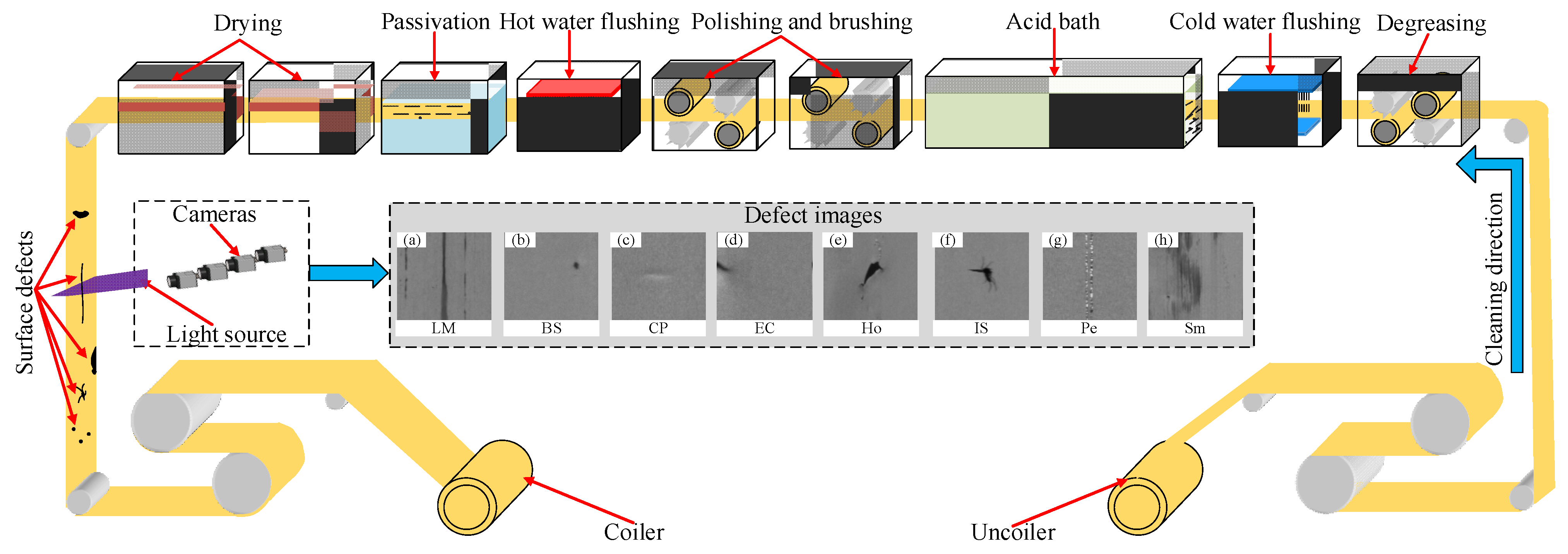
2. Surface Defect of Copper Strip

2.1. Classifications and Characteristics of Surface Defects

Surface defects of copper strip may occur in different process stages, such as cold rolling, annealing and cleaning. Multiple sets of high-speed cameras are usually installed at the end of the cleaning line to photograph the surface of the copper strip continuously, and the image acquisition process is shown in Figure 1. The surface defects must be accurately classified, identified and counted firstly during the practical production. The targeted defect control measures can then be formulated to improve the surface quality and product performance.
Eight classifications of defects, namely line mark (LM), black spot (BS), concave–convex pit (CP), edge crack (EC), hole (Ho), insect spot (IS), peeling (Pe), and smudge (Sm), were determined after long-term site tracking, sampling analysis, and technical exchanges in the copper strip production line. The morphology of the eight classifications of surface defects is shown in Figure 1, and the specific feature of these classifications of surface defects is presented in Table 1. The table reveals that the shapes and textures amongst the defects are not completely consistent, which is beneficial for defect recognition. However, some similarities are found between different defects; for example, EC and Ho show blocky features, which increases the difficulty of accurate defect recognition.

2.2. Surface Defect Dataset

The eight types of surface defect images mentioned above were collected on a domestic copper strip production line. The three types of defects of LM, CP, and EC after a period of production site tracking appeared relatively few times, collecting 157, 204, and 231, respectively. The collected number of other types of defect images was more than 300. This paper combines the image augmentation theory and practical environmental conditions that may occur to ensure even distribution of each type of defect image and randomly adopts five transformation methods shown in Table 2 (adding Gaussian noise, salt and pepper noise, angle rotation, brightness reduction, and enhancement) to expend the three aforementioned types of defect images, wherein each type was expended to 300.
The original image and the added noise are respectively assumed as f and n when adding noise to the image, and then the image after adding noise is expressed as Equation (1). If the noise type is Gaussian noise, then it should obey the normal distribution [21], and the probability density function of the noise n should satisfy the Equation (2); if the noise type is salt and pepper noise, then this type shows bright and dark spots in the image [22], and the probability density function of the noise n should satisfy Equation (3).
g = f + n
p ( n ) = 1 2 π σ e ( n μ ) 2 / ( 2 σ 2 )
where μ is the average value of noise n , and σ is the standard deviation of noise n .
p ( n ) = { p a p b 1 p a p b n = a n = b n a ,   n b
where 0 p a 1 , 0 p b 1 . If a > b , then the noise n = a is reflected as a light spot; if a < b , then the noise n = b is reflected as dark spots.
The centre of the image is the fixed point when the image is rotated, and the coordinate of any point in the original image is ( x 0 , y 0 ) . The coordinate after the rotation angle θ becomes ( x , y ) , and the calculation equation between the two is expressed as Equation (4).
[ x y ] = [ cos θ sin θ sin θ cos θ ] [ x 0 y 0 ] .
The brightness adjustment aims to increase or decrease uniformly the gray value of all pixels in the image. Assuming that the gray values in the original image are represented by Ω , Ω is the adjusted gray values, and the calculation equation between the two is expressed as Equation (5).
Ω = Ω × ( 1 + η )
where η is the brightness adjustment factor.
The surface defect dataset of the copper strip (YSU_CSC) in this paper is shown in Figure 2. This dataset contains 2400 surface defect images, and each defect has 300 images. The original image size is 200 × 200. The size of each image is unified to 224 × 224 after image pre-processing. A total of 70% of these images is used as the training set, half of the remaining 30% is the validation set and the other half is the test set. Training and validation sets are used for model training. The test set is used to assess the generalisation capability of the model, which does not participate in model training. The specific distribution of various types of defect images in the dataset is shown in Table 3.

3. Surface Defect Detection Model

Figure 3 shows the two steps for the detection model of surface defects. Step I: Discriminating the collected images initially is necessary to distinguish between the perfect and defect images. Step II: Classifying the defect images to their corresponding specific classification (LM, BS, CP, EC, Ho, IS, Pe, and Sm). The detection of surface defects can be realised through the two aforementioned steps.

3.1. Surface Defect Discrimination Model

This paper establishes a surface defect discrimination model based on the information difference of internal characteristics between perfect and defect images to realise the discrimination of the presence of image defects in step I. Since the collected original image is a gray image, the gray value of each internal pixel is Ω (0–255) for an original image. Perfect and defect images are respectively expressed as p and d. The distribution statistics of the gray values of all pixels in pending image f indicate that Equation (6) can determine whether f belongs to a perfect or defect image. Figure 4a shows the statistical results of the gray value distribution of a perfect image, and Figure 4b–i shows the statistical results of the gray value distribution of eight classifications of defect images. The figure reveals that the gray values of the perfect image are all clustered and distributed around the median value of 127.5, whilst a part of the gray values of defect image is distributed in the range of <100 and >200. Thus, the perfect and defect images can be quickly distinguished. Meanwhile, internal information amongst defect images from Figure 4b–i demonstrates strong similarity, which is difficult to classify using a simple model. Therefore, step II should be implemented to establish the surface defect recognition model.
f = { p ε 1 Ω ε 2 d Ω < ε 1 , Ω > ε 2
where ε 1 and ε 2 are discrimination coefficients, and their values are determined in accordance with the production site environment. The values in this paper are ε 1 = 100 and ε 2 = 200 .

3.2. Surface Defect Recognition Model of CNN

Traditional machine vision and deep learning can be used to realise automatic detection of copper strip surface defects. If traditional machine vision is used to extract and classify the defect feature, then endowing the model with high detection accuracy and strong capability of generalisation and anti-interference is difficult. At present, the convolution neural network (CNN) has made outstanding application performance in many engineering fields, such as the defect detection of the steel strip surface, fault diagnosis, and pattern recognition, with the rapid development of artificial intelligence and deep learning theory [23,24,25,26]. Therefore, this paper establishes the intelligent recognition model of copper strip surface defect based on the deep CNN, according to the defect images collected from the production site. The general structure of the model is shown in Figure 5. This structure mainly comprises an input layer of the image data, multiple convolutional layer, multiple pooling layer, fully connected neural network layer, and an output layer; the specific number of convolution and pooling layers should be determined in accordance with the specific problem. The feature information of surface defect is extracted after the multiple operations of convolution, pooling, and non-linear activation function mapping on the surface defect image of the copper strip. Finally, the probability of each type for a certain image is calculated through fully connected and output layers and realises defects classification.

3.3. Surface Defect Recognition Model of EfficientNet

At present, scholars have conducted many theoretical investigations regarding deep CNN. The resolution of the input image and the depth and width of the network are assumed to be the dominant factors that affect the model performance. Some studies have expanded the network structure based on the three aforementioned factors, such as common ResNet, DenseNet, and MobileNet [27,28,29]. These models only expanded the network on a single factor, which can improve the accuracy to a certain extent. However, blindly adding one dimension will complicate the model structure, and excessively large parameter values are prone to cause over-fitting [30,31], which is not beneficial to the establishment of the surface defect recognition model. Thus, this paper uses a new CNN model (EfficientNet) to investigate surface defect recognition. This model uses a composite zoom factor to expand the three dimensions of the width and depth of network and image resolution [32,33], which can reduce the complexity of the model under the premise of the same accuracy. The expression of the zoom factor is Equation (7).
{ depth : d = α ϕ width : w = β ϕ resolution : r = γ ϕ s . t . α · β 2 · γ 2 2 α 1 , β 1 , γ 1
where d , w , and r are the zoom factors of width, depth, and resolution, respectively; ϕ is the source control factor, which regulates the resources available for model zoom (computing power); and α , β , and γ are the resource allocation coefficients that can be determined by grid search, and these resources are allocated to width, depth, and resolution, respectively. The model accuracy can be optimised by continuously adjusting the zoom factor of d , w , and r without increasing the number of model parameters.
The EfficientNet model is essentially an optimization problem [33]. The accuracy of the model is improved by continuously optimizing the combination of depth d , width w , and resolution r . The optimization process is expressed as Equation (8).
max d , w , r A c c u r a c y ( N ( d , w , r ) ) s . t . N ( d , w , r ) = i = 1 s F ^ i d L ^ i ( X r · H ^ i , r · W ^ i , w · C ^ i ) Memory ( N ) target _ memory FLOPS ( N ) target _ flops
where N is the network model; i is the component of the network model; s is the total number of components; F ^ , L ^ i , H ^ i , W ^ i , and C ^ i are predefined parameters in network; F ^ is the predefined network layer structure, L ^ i is the predefined number of layers, H ^ i and W ^ i are the predefined resolution, and C ^ i is predefined number of channels; X is the adjustment factor; Memory(N) is the number of parameters of the network; FLOPS(N) is the amount of floating point calculation on the network; is the model building operation; target_memory is the threshold value of the parameter quantity; target_flpos is the threshold value of the floating-point calculation quantity; and max Accuracy is the maximum accuracy of the model (objective function value).
This paper uses EfficientNet to establish an intelligent recognition model for the copper strip surface defects to reduce the model parameters, increase the calculation speed and combine the resolution of surface defect images. The model structure comprises one image data input layer, two Conv convolutional layers, sixteen MBConv mobile inverted bottleneck convolution module layers, one pooling layer and three fully connected layers. The overall structure of the model is shown in Figure 6. The main structure of the model is the MBConv module. The output channel dimension is changed by 1 × 1 point-by-point convolution, according to the expansion ratio. A 1 × 1 point-by-point convolution is used after one deep convolution to restore the original dimension, and the internal activation function is Swish [34,35]. The module structure of MBConv1 and MBConv6 is shown in Figure 7.

4. Experiments and Results

4.1. Experimental Method

The model training experiment adopts the transfer learning strategy and then analyses the influence of the model structure and parameters on the recognition accuracy and calculation speed of surface defect images. Firstly, the model is by the ImageNet dataset after several experimental comparisons and analysis, helping the model reach a certain accuracy. The seven last layers (three fully connected and four convolutional layers) are then retrained by the YSU_CSC dataset. Thus, the model presents good recognition performance for surface defects. Figure 8 shows the training strategy of the model. As shown in Figure 9, this paper also uses three other common deep CNN algorithms (VGG16, MobileNetV2, and ResNet50) to establish the corresponding surface defect recognition model for comparison.

4.2. Experimental Results and Analysis

The error loss function value and the accuracy of the model training process after 2000 epochs of training are shown in Figure 10. It can be seen from Figure 10g,h that the error loss of the model on the training and validation sets respectively reached 0.25 and 0.34, and the overall training process performed relatively smoothly, indicating the good learning capability of the model. The accuracy of the training and validation sets respectively reached 0.93 and 0.95 after the training process, which indicated that the model had a certain generalisation capability. As shown in Figure 10a–f, compared with the other three models, the training process of the model in this paper is more stable, and there are no problems, such as over fitting or local oscillation. This also shows the effectiveness of the training strategy in this paper.
The model was used to predict the defect images of the ‘unseen’ testing set to further verify the accuracy and generalisation capability. Meanwhile, the performance of three recognition models (VGG16, MobileNetV2, and ResNet50) was compared on the same testing set, and the result is shown in Table 4. Among these results, the recognition accuracies of the VGG16, MobileNetV2, and ResNet50 are 75.27%, 65.83%, and 82.78%, respectively. Compared with the three models, the accuracy of the model proposed in this paper is the highest at 93.05%. Compared with traditional methods [9,36], the accuracy of the model and the ability to recognize the number of defect classifications are improved. The average recognition times of VGG16, MobileNetV2, and ResNet50 for a single defect image are 2412, 165, and 1205 ms, respectively. The model in this paper is 197 ms, which is similar to MobileNetV2. Considering the accuracy and the recognition speed, the model proposed in this paper is the best and can meet the engineering requirements (industrial production generally requires that the detection accuracy of the model should be higher than 90%).
This paper conducts a visual analysis of defect image classification and recognition results on the testing set to investigate the classification mechanism of the model for defect images. Figure 11 shows the recognition probability of eight types of defect images in the testing set. The blue and red balls respectively represent the recognition probabilities of correct and incorrect classification. The figure shows that the model has a good overall recognition performance for LM, CP, and Sm on the testing set with low error rates of 0%, 4.44%, and 2.22%, respectively. The recognition error rates of BS, Ho, and IS are relatively high, which are 8.89%, 15.56%, and 11.11%, respectively.
Figure 12 shows the class activation mapping (CAM) of the model for eight defect classifications in this paper. The deep red colour area in the figure places considerable importance for model defect classification. It can be seen from the figure that the model has good overall recognition performance for defect features. The LM and Pe both present linear decision areas, but significant differences are found between the two defects, which are easily distinguished. The decision areas of BS, EC, Ho, and IS present a clustering block range with a certain similarity, which easily makes them susceptible to the influence of the original image feature, causes confusion, and leads to misidentification. The decision area of CP and Sm has a certain degree of dispersibility. The CP and Sm respectively show local and global dispersions. This finding indicates that the proposed model in this paper has indeed learned the key feature information from various defect classifications.
A confusion matrix of training and testing sets is established to further analyse the reason for incorrect model recognition, which is shown in Figure 13. Figure 13a,b reveals that the longitudinal and horizontal axes respectively represent the true classification and model prediction classification labels. The value on the diagonal axis represents the accuracy of the recognition result, whilst that deviating from the diagonal represents the error rate of the recognition result. The depth of the colour in this figure corresponds to the value of the correct rate. The diagonal colour reveals that the proposed model in this paper has a good capability of learning and generalisation. By contrast, BS is easily identified as CP, Ho is easily identified as BS or EC, and IS is easily identified as Ho from Figure 13b. Artificial comparison of these actual defect images reveals the similar morphology feature of some images, which easily causes confusion. Future research can focus on increasing the amount of defect image data and formulating detailed classification standards for defect images to further improve the model recognition accuracy of surface defects.

5. Conclusions

  • Combining the practical requirement, the common surface defects of copper strip were divided into 8 classifications: line mark (LM), black spot (BS), concave–convex pit (CP), edge crack (EC), hole (Ho), insect spot (IS), peeling (Pe), and smudge (Sm). Image data were collected in a production line, and a dataset of copper strip surface defects was established (YSU_CSC).
  • The gray values of the perfect image clustered and distributed around the median value of 127.5, whilst a part of the gray values of the defect image was distributed in the range of <100 and >200. The perfect and defect images could be quickly distinguished.
  • Compared with the performance of VGG16, MobileNetV2, and ResNet50 on the same testing set, the surface defect recognition model of copper strip based on the EfficientNet convolutional neural network had the highest accuracy, reaching 93.05%. The average recognition time of a single defect image was 197 ms. The model has a good generalisation capability, and its calculation speed is fast, which can meet the actual engineering requirements and has the best overall performance.
  • On the testing set, the model improved the overall recognition performance on LM, CP, and Sm, with low error rates of 0%, 4.44%, and 2.22%, respectively. The defect recognition error rates for the three classifications of BS, Ho, and IS were relatively high at 8.89%, 15.56%, and 11.11%, respectively. The CAM shows that the model learned the key feature information for various classifications of defects. Consideration will be given in the future to further improve the overall performance of the model from three aspects: increasing the number of defect image data, subdividing similar defective images, and improving the model structure.

Author Contributions

Conceptualisation, Y.X. and D.W.; methodology, Y.X. and D.W.; writing—original draft preparation, Y.X. and D.W.; writing—review and editing, Y.X. and B.D.; supervision, H.Y. and B.D.; funding acquisition, D.W. and H.L. All authors have read and agreed to the published version of the manuscript.

Funding

This work was supported by the National Natural Science foundation of China (Grant No. 52074242), and the High-end Talents and “Giant Plan” Innovation Team of Hebei Province. (Grant No. 2019).

Institutional Review Board Statement

Not applicable.

Informed Consent Statement

Not applicable.

Data Availability Statement

Not applicable.

Conflicts of Interest

The authors declare no conflict of interest.

Abbreviations and Symbols

The following abbreviations and symbols are used in this manuscript:
AbbreviationDescription
LMLine Mark
BSBlack Spot
CPConcave–convex Pit
ECEdge Crack
HoHole
ISInsect Spot
PePeeling
SmSmudge
YSU_CSCA Surface Defect Dataset of Copper Strip
CNNConvolution Neural Network
MBConvMobile Inverted Bottleneck Convolution Module Layers,
VGGVisual Geometry Group Network
MobileNetEfficient Convolutional Neural Networks for Mobile Vision Applications
ResNetResidual Network
EfficientNetVariable Model Scale Convolution Neural Network
CAMClass Activation Mapping
SymbolsDescription
f Original image
n The added noise
g Image after adding noise
p ( n ) Probability density function of noise
( x 0 , y 0 ) Coordinate of any point in the original image
( x , y ) The coordinate after the rotation angle θ becomes
Ω Gray values in the original image
Ω Gray value after brightness adjustment
η Brightness adjustment factor
p Perfect images
d Defect images
ε 1 , ε 2 Discrimination coefficients
d , w , r Zoom factors of width, depth, and resolution
α , β , γ Resource allocation coefficients that can be determined by grid search, and these resources are allocated to width, depth, and resolution
NNetwork model
F ^ Predefined network layer structure
L ^ i Predefined number of layers
H ^ i , W ^ i Predefined resolution
C ^ i Predefined number of channels
X Adjustment factor
Memory(N) Number of parameters of the network
FLOPS(N)Amount of floating-point calculation on the network
Model building operation
taget_memoryThreshold value of the parameter quantity
target_flposThreshold value of the floating-point calculation quantity
max AccuracyMaximum accuracy of the model (objective function value)

References

  1. Jin, P.; Liu, C.M.; Yu, X.D.; Yuan, F.S. Present situation of Chinese copper processing industry and its development trend. Nonferrous Met. Eng. Res. 2015, 36, 32–35. [Google Scholar]
  2. Li, Y.; Wang, A.J.; Chen, Q.S.; Liu, Q.Y. Influence factors analysis for the next 20 years of Chinese copper resources demand. Adv. Mater. Res. 2013, 734–737, 117–121. [Google Scholar] [CrossRef]
  3. Zhang, W.Q.; Zheng, C.F. Surface quality control and technical actuality of copper and copper alloy strip. Nonferrous Met. Mater. Eng. 2016, 37, 125–131. [Google Scholar] [CrossRef]
  4. Zhang, Y.J. Discussion on surface quality control of copper sheet and strip. Nonferrous Met. Process. 2005, 34, 27–29. [Google Scholar]
  5. Song, Q. Applications of machine vision to the quality test of copper strip surfaces. Shanghai Nonferrous Met. 2012, 77–80. [Google Scholar] [CrossRef]
  6. Yuan, H.Z.; Fu, W.; Guo, Y.K. An algorithm of detecting surface defects of copper plating based on dynamic threshold. J. Yanshan Univ. 2010, 34, 336–339. [Google Scholar] [CrossRef]
  7. Shen, Y.M.; Yang, Z.B. Techniques of machine vision applied in detection of copper strip surface’s defects. Electron. Meas. Technol. 2010, 33, 65–67. [Google Scholar] [CrossRef]
  8. Zhang, X.W.; Ding, Y.Q.; Duan, D.Q.; Gong, F.; Xu, L.Z.; Shi, A.Y. Surface defects inspection of copper strips based on vision bionic. J. Image Graph. 2011, 16, 593–599. [Google Scholar]
  9. Li, J.H. Research on Key Technology of Surface Defect Detection in Aluminum/Copper Strip. Master’s Thesis, Henan University of Science and Technology, Luoyang, China, 2019. [Google Scholar]
  10. Meng, F.M. Development of Copper Strip Defect Online Detection System Based on ARM and DSP. Master’s Thesis, China Jiliang University, Hangzhou, China, 2019. [Google Scholar] [CrossRef]
  11. Zhang, X.W.; Gong, F.; Xu, L.Z. Inspection of surface defects in copper strip using multivariate statistical approach and SVM. Inter. J. Comput. Appl. Technol. 2012, 43, 44–50. [Google Scholar] [CrossRef]
  12. Peres, R.S.; Jia, X.D.; Lee, J.; Sun, K.Y.; Colombo, A.W.; Barata, J. Industrial artificial intelligence in industry 4.0-systematic review, challenges and outlook. IEEE Access 2020, 8, 220121–220139. [Google Scholar] [CrossRef]
  13. Song, K.C.; Yan, Y.H. A noise robust method based on completed local binary patterns for hot-rolled steel strip surface defects. Appl. Surf. Sci. 2013, 285, 858–864. [Google Scholar] [CrossRef]
  14. He, Y.; Song, K.C.; Meng, Q.G.; Yan, Y.H. An end-to-end steel surface defect detection approach via fusing multiple hierarchical features. IEEE Trans. Instrum. Meas. 2019, 64, 1493–1504. [Google Scholar] [CrossRef]
  15. Saiz, F.A.; Serrano, I.; Barandiaran, I.; Sanchez, J.R. A robust and fast deep learning-based method for defect classification in steel surfaces. In Proceedings of the 9th International Conference on Intelligent Systems (IS), Funchal, Portugal, 25–27 September 2018; pp. 455–460. [Google Scholar]
  16. Xiang, K.; Li, S.S.; Luan, M.H.; Yang, Y.; He, H.M. Aluminum product surface defect detection method based on improved Faster RCNN. Chin. J. Sci. Instrum. 2021, 42, 191–198. [Google Scholar] [CrossRef]
  17. Zheng, X.; Huang, D.J. Defect detection on aluminum surfaces based on deep learning. J. East. China Norm. Univ. (Nat. Sci.) 2020, 105–114. [Google Scholar] [CrossRef]
  18. Ye, G.; Li, Y.B.; Ma, Z.X.; Cheng, J. End-to-end aluminum strip surface defects detection and recognition method based on ViBe. J. Zhejiang Univ. (Eng. Sci.) 2020, 54, 1906–1914. [Google Scholar] [CrossRef]
  19. Gao, Y.P.; Gao, L.; Li, X.Y.; Yan, X.G. A semi-supervised convolutional neural network-based method for steel surface defect recognition. Robot. Comput.-Integr. Manuf. 2020, 61, 101825. [Google Scholar] [CrossRef]
  20. He, Y.; Song, K.C.; Dong, H.W.; Yan, Y.H. Semi-supervised defect classification of steel surface based on multi-training and generative adversarial network. Opt. Lasers Eng. 2019, 122, 294–302. [Google Scholar] [CrossRef]
  21. Naseri, M.; Beaulieu, N.C. Fast simulation of additive generalized Gaussian noise environments. IEEE Commun. Lett. 2020, 24, 1651–1654. [Google Scholar] [CrossRef]
  22. Thanh, D.N.H.; Hai, N.H.; Prasath, V.B.S.; Hieu, L.M.; Tavares, J.M.R.S. A two-stage filter for high density salt and pepper denoising. Multimed. Tools Appl. 2020, 79, 21013–21035. [Google Scholar] [CrossRef]
  23. Lee, S.Y.; Tama, B.A.; Moon, S.J.; Lee, S. Steel surface defect diagnostics using deep convolutional neural network and class activation map. Appl. Sci. 2019, 9, 5449. [Google Scholar] [CrossRef] [Green Version]
  24. Wang, D.C.; Xu, Y.H.; Duan, B.W.; Wang, Y.M.; Song, M.M.; Yu, H.X.; Liu, H.M. Intelligent recognition model of hot rolling strip edge defects based on deep learning. Metals 2021, 11, 223. [Google Scholar] [CrossRef]
  25. Piltan, F.; Prosvirin, A.E.; Jeong, I.; Im, K.; Kim, J.M. Rolling-element bearing fault diagnosis using advanced machine learning-based observer. Appl. Sci. 2019, 9, 5404. [Google Scholar] [CrossRef] [Green Version]
  26. Zhang, X.L.; Cheng, L.; Hao, S.; Gao, W.Y.; Lai, Y.J. Optimization design of RBF-ARX model and application research on flatness control system. Optim. Control Appl. Methods 2017, 38, 19–35. [Google Scholar] [CrossRef]
  27. He, K.M.; Zhang, X.Y.; Ren, S.Q.; Sun, J. Deep residual learning for image recognition. In Proceedings of the IEEE Conference on Computer Vision and Pattern Recognition (CVPR), Seattle, WA, USA, 27–30 June 2016; pp. 770–778. [Google Scholar] [CrossRef] [Green Version]
  28. Huang, G.; Liu, Z.; Laurens, V.D.M.; Weinberger, K.Q. Densely connected convolutional networks. In Proceedings of the IEEE Conference on Computer Vision and Pattern Recognition (CVPR), Honolulu, HI, USA, 21–26 July 2017; pp. 2261–2269. [Google Scholar] [CrossRef] [Green Version]
  29. Sandler, M.; Howard, A.; Zhu, M.; Zhmoginov, A.; Chen, L. MobileNetV2: Inverted residuals and linear bottlenecks. In Proceedings of the IEEE/CVF Conference on Computer Vision and Pattern Recognition (CVPR), Salt Lake City, UT, USA, 18–23 June 2018; pp. 4510–4520. [Google Scholar] [CrossRef] [Green Version]
  30. Alhichri, H.; Alsuwayed, A.; Bazi, Y.; Ammour, N.; Alajlan, N.A. Classification of remote sensing images using EfficientNet-B3 CNN Model with Attention. IEEE Access 2021, 9, 14078–14094. [Google Scholar] [CrossRef]
  31. Duong, L.T.; Nguyen, P.T.; Di Sipio, C.; Di Ruscio, D. Automated fruit recognition using EfficientNet and MixNet. Comput. Electron. Agric. 2020, 171, 105326. [Google Scholar] [CrossRef]
  32. Tan, M.X.; Le, Q.V. Efficientnet: Rethinking model scaling for convolutional neural networks. arXiv 2019, arXiv:1905.11946. [Google Scholar]
  33. Bazi, Y.; Al Rahhal, M.M.; Alhichri, H.; Alajlan, N. Simple yet effective fine-tuning of deep CNNs using an auxiliary classification loss for remote sensing scene classification. Remote Sens. 2019, 11, 2908. [Google Scholar] [CrossRef] [Green Version]
  34. Zhou, Z.J.; Zhang, B.F.; Yu, X. Infrared handprint classification using deep convolution neural network. Neural. Process. Lett. 2021, 53, 1065–1079. [Google Scholar] [CrossRef]
  35. Lyu, Y.Q.; Jiang, J.; Zhang, K.; Hua, Y.L.; Cheng, M. Factorizing and reconstituting large-kernel MBConv for lightweight face recognition. In Proceedings of the 2019 IEEE/CVF International Conference on Computer Vision Workshop (ICCVW), Seoul, Korea, 27 October–2 November 2019; pp. 2689–2697. [Google Scholar] [CrossRef]
  36. Gao, F.; Li, Z.; Xiao, G.; Yuan, X.Y.; Han, Z.G. An online inspection system of surface defects for copper strip based on computer vision. In Proceedings of the 2012 5th International Congress on Image and Signal Processing (CISP), Chongqing, China, 16–18 October 2012; pp. 1200–1204. [Google Scholar] [CrossRef]
Figure 1. Image acquisition process of surface defects of copper strip: (a) LM, (b) BS, (c) CP, (d) EC, (e) Ho, (f) IS, (g) Pe, and (h) Sm.
Applsci 11 08945 g001
Figure 2. Surface defect dataset of copper strip (YSU_CSC).
Applsci 11 08945 g002
Figure 3. Surface defect detection model process.
Applsci 11 08945 g003
Figure 4. Statistical results of gray value distribution of perfect and defect images: (a) perfect image, (b) LM, (c) BS, (d) CP, (e) EC, (f) Ho, (g) IS, (h) Pe, and (i) Sm.
Applsci 11 08945 g004
Figure 5. General structure of the surface defect CNN model.
Applsci 11 08945 g005
Figure 6. Surface defect EfficientNet recognition model.
Applsci 11 08945 g006
Figure 7. MBConv block: (a) MBConv1, (b) MBConv6.
Applsci 11 08945 g007
Figure 8. Training strategy of the model.
Applsci 11 08945 g008
Figure 9. Recognition models are established by other three CNNs: (a) VGG16, (b) MobileNetV2, and (c) ResNet50.
Applsci 11 08945 g009
Figure 10. Error loss and accuracy of the recognition models: (a,b) VGG16, (c,d) MobileNetV2, (e,f) ResNet50, and (g,h) EfficientNet.
Applsci 11 08945 g010aApplsci 11 08945 g010b
Figure 11. Proposed model recognition result probability of each defect image on the testing set: (a) LM, (b) BS, (c) CP, (d) EC, (e) Ho, (f) IS, (g) Pe, and (h) Sm.
Applsci 11 08945 g011aApplsci 11 08945 g011b
Figure 12. Class activation maps of surface defects localised by the proposed model: (a) original defect image; (b) class activation maps.
Applsci 11 08945 g012
Figure 13. Confusion matrix of the training and testing sets by the proposed model: (a) training set, (b) testing set.
Applsci 11 08945 g013
Table 1. Characteristics of surface defects.
ClassificationsCharacteristics
LMSingle or multiple lines appear on the surface, with continuous or intermittent distribution and different lengths.
BSSingle or multiple round black spots on the surface, usually single spot point is common.
CPPits or bulges of different sizes on the surface.
ECCracks on the sides of the two sides extend from the outside to the inside.
HoHoles with different sizes and irregular shapes on the surface.
ISMost are embedded in the surface of copper strip, with insect appearance.
PeSerious upwarp appear on the surface.
SmIrregular dispersive residue marks appear on the surface.
Table 2. Surface defect image data enlargement.
Defects ClassificationImage Augmentation
Original ImageGaussian NoiseSalt Pepper NoiseAngle RotationBrightness ReductionBrightness Enhancement
LM Applsci 11 08945 i001 Applsci 11 08945 i002 Applsci 11 08945 i003 Applsci 11 08945 i004 Applsci 11 08945 i005 Applsci 11 08945 i006
CP Applsci 11 08945 i007 Applsci 11 08945 i008 Applsci 11 08945 i009 Applsci 11 08945 i010 Applsci 11 08945 i011 Applsci 11 08945 i012
EC Applsci 11 08945 i013 Applsci 11 08945 i014 Applsci 11 08945 i015 Applsci 11 08945 i016 Applsci 11 08945 i017 Applsci 11 08945 i018
Table 3. Distribution of surface defect images in the training, validation, and testing sets.
DatasetLMBSCPECHoISPeSmTotal
Training set2102102102102102102102101680
Validation set4545454545454545360
Testing set4545454545454545360
Total3003003003003003003003002400
Table 4. Comparison of results of different models on the testing set.
Recognition ModelsTesting Set Accuracy (%)Recognition Time of Single Defect Image (ms)
VGG1675.272412
ResNet5082.781205
MobileNetV265.83165
Ours method93.05197
Publisher’s Note: MDPI stays neutral with regard to jurisdictional claims in published maps and institutional affiliations.

