Article

Prediction of Beck Depression Inventory Score in EEG: Application of Deep-Asymmetry Method

1
Department of IT Convergence Engineering, Gachon University, Sungnam-si 13306, Korea
2
Department of Computer Engineering, Gachon University, Sungnam-si 13306, Korea
*
Author to whom correspondence should be addressed.
Appl. Sci. 2021, 11(19), 9218; https://doi.org/10.3390/app11199218
Submission received: 31 August 2021 / Revised: 25 September 2021 / Accepted: 29 September 2021 / Published: 3 October 2021
(This article belongs to the Special Issue Deep Convolutional Neural Networks)

Abstract

:
There is ongoing research on using electroencephalography (EEG) to predict depression. In particular, the deep learning method in which brain waves are used as inputs of a convolutional neural network (CNN) is being widely researched and has shown remarkable performance. We built a regression model to predict the severity score (Beck Depression Inventory [BDI]) of depressed patients as an extension of the deep-asymmetry method, which has shown promising performance in depression classification. Predicting the severity of depression is very important because the treatment and coping methods are different for each severity level. We imaged brain waves using the deep-asymmetry method, used them to train a two-dimensional CNN-based deep learning model, and achieved satisfactory performance. The EEG image-based CNN approach will make an important contribution to creating a highly interpretable model for predicting depression in the future.

1. Introduction

Clinical decision support systems (CDSSs) are emerging with the dawn of the modern data era [1]. A CDSS can help clinicians make the most rational decisions based on clinical information when diagnosing or treating diseases [2]. In particular, a non-knowledge-based CDSS provides decision support by learning patterns in data using clinical-data-based data analysis, machine learning, and deep learning.
Research in the field of brain diseases and clinical decision support systems is ongoing. Major depressive disorder (MDD), a critical brain disease, is one of the most common mental disorders; according to the World Health Organization (WHO), approximately 10–15% of the world’s population will experience depression at least once in their lifetime [3]. Depression not only seriously interferes with the afflicted persons’ social life but also leads to serious problems such as suicide if left untreated for long periods of time. However, a large number of patients do not visit a medical institution because they are unaware that they have depression, or even if they do, they are unaware of its severity.
The diagnosis of depression is most commonly performed through psychological diagnostic methods in consultation with a psychiatrist [4]. This disorder is diagnosed by a psychiatrist based on the diagnostic criteria presented in the Diagnostic and Statistical Manual of Mental Disorders (DSM-V) [5]. In addition, auxiliary questionnaire-based methods such as the Beck Depression Inventory [6] and the Hamilton Depression Rating Scale [7] can be used in combination. However, these psychological methods may lead to different diagnostic results and misdiagnoses depending on the expertise of a psychiatrist. In particular, on using these methods, symptoms of depression may appear as symptoms of diseases other than depression [8].
In light of this, a CDSS based on objective data is one of the most appropriate solutions for diagnosing depression and brain diseases. Traditionally, brain diseases are diagnosed through medical data-based research using methods such as computed tomography (CT) [9], magnetic resonance imaging (MRI) [10], and functional magnetic resonance imaging (fMRI) [11].
Among them, electroencephalography (EEG) is being widely researched because it is relatively low-cost and easy to implement compared with the methods described above. In addition to depression, many brain diseases have been studied using EEG analysis. Studies have been conducted to predict dementia [12], schizophrenia [13], epilepsy [14], etc., using EEG. In particular, various attempts have been made to identify biomarkers of depression through EEG analysis [15]. Decreased frontal lobe activity in EEG [16] and alpha-hemispheric asymmetry [17] have been identified as representative biomarkers of depressive EEG.
In these studies, incorporating machine learning techniques has led to significant progress in EEG-based depression prediction. The machine learning technique enables the development of effective models for classifying depressed patients and healthy controls using various features extracted from brain waves. Mumtaz presented a machine learning model to classify MDD patients and healthy controls using different EEG frequency bands and EEG alpha hemisphere asymmetry as derived features [18]. Similarly, Muhato et al. constructed variables by separately characterizing the alpha 1 and alpha 2 bands based on band power, asymmetry characteristics, and alpha band power and built a machine learning model based on this characterization [19]. In addition, Muhato et al. presented a machine learning classification model that uses both linear characteristics such as band power and hemispheric asymmetry characteristics and nonlinear characteristics such as relative wavelet energy and wavelet entropy [20].
In addition, deep learning techniques have been applied to diagnose patients with depression. Machine learning techniques entail detailed feature extraction and feature-selection techniques. Deep learning techniques have been used extensively in the field of medical diagnosis as they have the ability to learn important characteristics by learning automatically based on raw data. It is particularly noteworthy that many deep learning model architectures use convolutional neural network (CNN)-based layers. There are two main approaches to applying CNNs in the field of EEG. First, there is a method of providing raw EEG data to a CNN in the form of time series data. For example, Acharya et al. presented a model to classify depressed patients and healthy controls using EEG signals and a 13-layer deep CNN model [21]. Mumtaz et al. proposed the use of a one-dimensional CNN for raw EEG signals and a model combining a CNN and long short-term memory (LSTM) [22].
Another approach is to visualize important characteristics within the EEG and present it to the model in the form of an image. Kwon et al. obtained spectrograms using the short-time Fourier transform (STFT) to classify depressed patients and healthy controls and presented a model for pre-screening depressed patients using low channels [23]. Kwon et al. applied STFT-based prefrontal EEG images to VGG16, one of the latest deep learning architectures, to achieve high EEG classification performance [24].
Li et al. presented a deep learning approach for recognizing mild depression using a functional connectivity matrix and CNN [25]. Li et al. proposed applying transfer learning together with a feature vector and RGB image as CNN-based model inputs with the goal of recognizing mild depression [26]. Saeedi et al. presented a deep learning classification model comprising a CNN and LSTM based on the effective connectivity between channels in EEGs [27]. For a decision support system for MDD detection, Loh et al. achieved the highest level of classification performance with a deep learning method using an image converted from an STFT-based spectrogram and an 8-layer CNN [28].
In particular, the deep-asymmetry method [29] used in this study is a method for training a deep learning model based on a CNN by converting the alpha asymmetry, a representative biomarker of depression, into a matrix-type image. Consequently, patients and healthy controls were classified with high accuracy.
However, the above-mentioned cases were limited to distinguishing between patients with depression and healthy controls. Depression is divided into several stages depending on its severity. The Beck Depression Inventory (BDI) [6] is one of the representative indicators of depression severity. The BDI consists of 21 sentences covering the cognitive, emotional, motivational, and physical symptoms of depression. It was first developed in 1961 and is widely used worldwide. It is scored by determining the total score of the responses to 21 sentences, and 0–13 is considered minimal depression, 14–19 mild depression, 20–28 moderate depression, and 29–63 severe depression. Furthermore, depression has different symptoms depending on its severity, and treatment and response methods are also different. Therefore, it is important to determine the severity of depression as well as to identify depression.
We considered AVEC 2013 [30] and 2014 [31] as part of the related research. The purpose of this subtask was to predict BDI scores using the presented video and audio sets. Several studies using this dataset have been conducted. Zhu et al. presented a deep learning method based on a co-tuning layer that simultaneously captures facial appearance and dynamics, resulting in a MAE of 7.58 (AVEC2013) and a MAE of 7.47 (AVEC2014) [32]. Melo et al. presented a deep learning architecture to predict depression levels through distribution learning and obtained MAEs of 6.30 (AVEC 2013) and 6.15 (AVEC2014) [33].
However, very few studies have presented a model predicting the severity of depression, such as the BDI, based on EEGs. We present a BDI regression model based on EEG as a follow-up study of the deep-asymmetry method validated by the existing depression patient classification model. We present a model for predicting the BDI by applying the deep asymmetry methodology, which has shown excellent performance in the classification of patients with MDD. EEGs are imaged using the asymmetry characteristic, a major biomarker of depression, and such images are used as inputs to a convolutional network. Models were tested on public datasets and compared with the most common baseline models. Figure 1 schematically illustrates the entire pipeline used in this study.

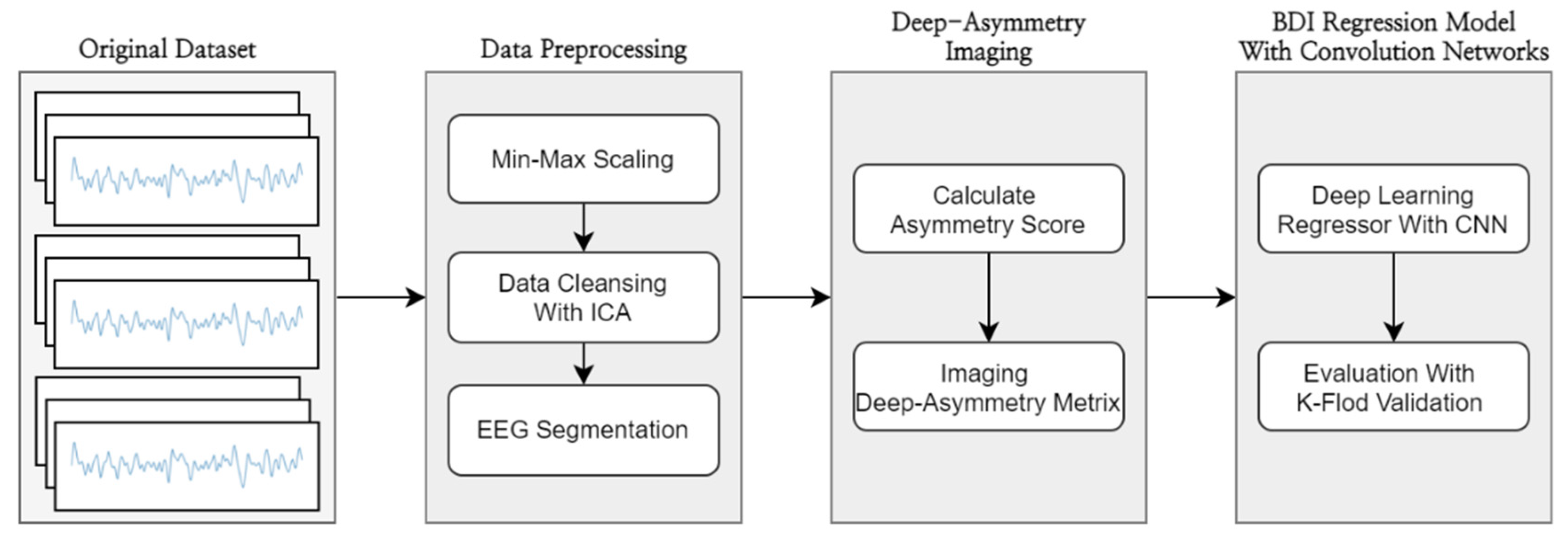
2. Materials and Methods

2.1. Dataset

We used the open dataset used in the study by Cavanagh et al. [34]. Data were provided by Openneuro [35]. Data were collected from 2008 to 2010 at the John JB Allen lab at the University of Arizona. The recruitment criteria for participants were as follows: (1) 18 to 25 years of age, (2) no history of head trauma and seizures, and (3) no use of antipsychotics. Data were obtained from a probabilistic choice task involving 122 college students. The dataset corresponded to 74 male participants (mean age 18 ± 1 years) and 47 female participants (mean age, 18 ± 1 years). Participants’ BDI was distributed with a mean of 9.52 and a standard deviation of 10.50. All participants provided written informed consent, and the study was approved by the University of Arizona. EEGs were acquired at a sampling rate of 500 Hz through the Synamps system and passed through a band-pass filter of 0.5 to 100 Hz, measured using 64 Ag/AgCI electrodes.

2.2. Data Preprocessing

We selected the channel based on the international 10–20 system [36] among the EEG channels configured in the dataset to apply the deep asymmetry methodology [29] devised by us. Frontal (Fp1, Fp2, F7, F3, Fz, F4, F8), central (C3, Cz, C4), parietal (P7, P3, Pz, P4, P8), occipital (O1, O2), and temporal (T7, T8) channels, a total of 19, were selected.
The EEG data were normalized using the min-max normalization method [37] so that the amplitude scale between each channel could be similarly matched. Min-max normalization is the most common method for normalizing data, and for all channels, the minimum value is 0 and the maximum value is 0.
In addition, we used an independent signal analysis (ICA) method to reduce noise and artifacts in the EEG data and extract features. This method is considered effective for the cleansing and feature extraction of EEG signals [38]. We preprocessed the EEG using FastICA [39].
We used data segmentation to increase the number of samples in the dataset. A small number of samples in the dataset creates problems while training the model. Therefore, we used a method of dividing a sample of data into meaningful segments. This is a potential approach to address data quantitative limitations [12] and has been adopted in existing EEG studies [22,27]. We divided each dataset into small epochs (5120 samples) with a window size of 10 s (no overlab). Each epoch was assigned the same value.

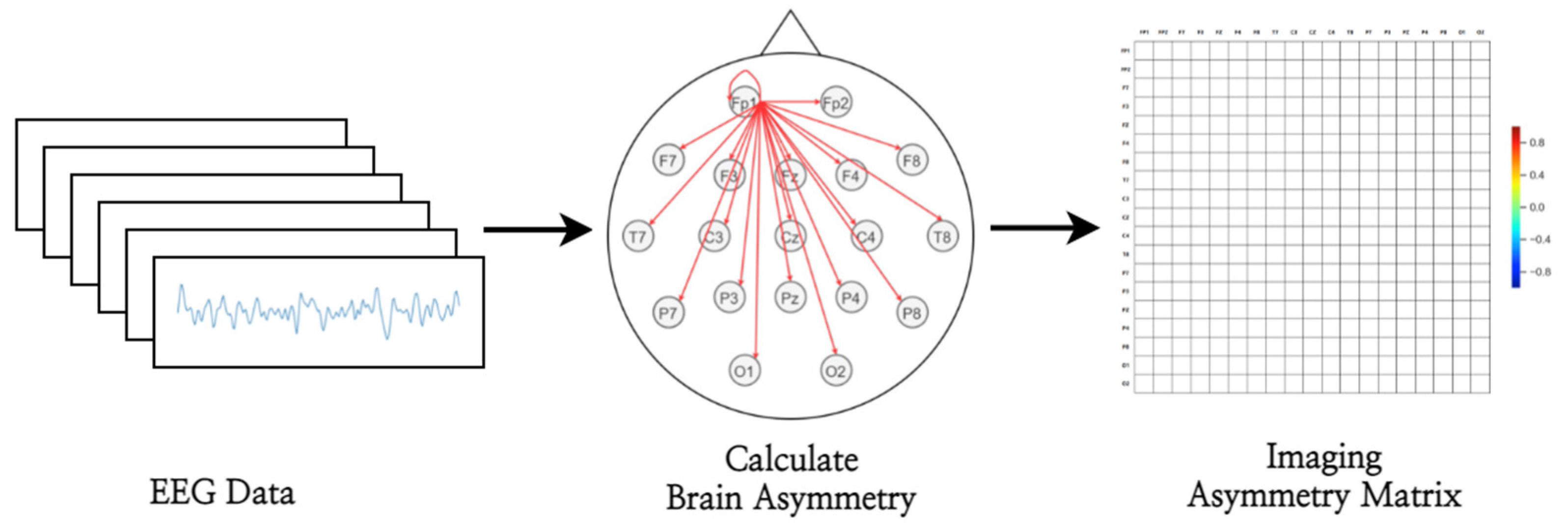
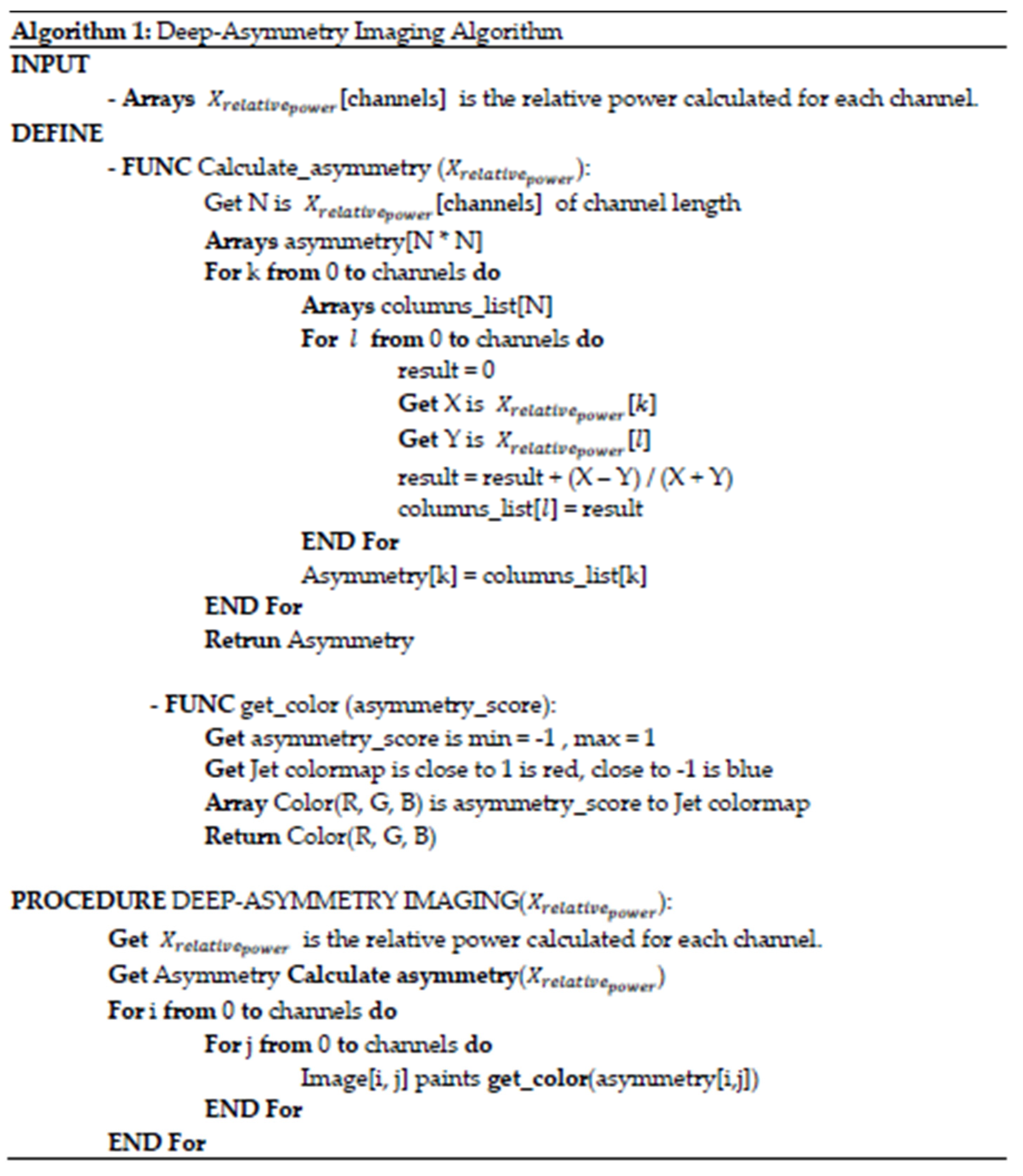
2.3. Deep-Asymmetry Imaging

Deep-asymmetry imaging shows the degree of asymmetry between EEG channels as a matrix visualization. We used this visualization method to develop a regression model to predict the severity of depression.
The deep-asymmetry visualization method involves calculating asymmetry scores between channels and visualizing the calculated scores in a matrix form. Figure 2 illustrates our proposed deep-asymmetry visualization method.

2.3.1. Brain Asymmetry Score Calculator

The inter-channel asymmetry score was obtained using the difference between the relative powers of the EEG signals between each channel. The power spectrum of the EEG signal was calculated using Welch’s periodic diagram [40]. This was used to obtain power spectral density S. The window size was set to twice the reciprocal of the low frequency of the frequency band of interest, and the power spectrum was obtained as 50% overlab. Using this, the calculated frequency band power spectral density was obtained using Simpson’s method [41]. Equation (1) is used to calculate the relative power of a given channel in the target frequency band, where f 1 and f 2 denote the lowest and highest frequencies in the band, respectively. For example, if the relative EEG signal power of the alpha wave (8–13 Hz) is calculated, f 1 = 8 and f 2 = 13. The power spectral densities at channel are denoted as S c h 1 .
Rp ch 1 = f = 8 f = 13 S c h 1 f = 0.5 Hz 30 Hz S c h 1
The relative power of each channel thus obtained was used to calculate the difference in the relative power of the two channels for each pair of channels. Equation (2) shows an example of the expression used to calculate the asymmetric score of channels 1 and 2. We computed the asymmetry scores for each channel. Figure 3 shows an example of our asymmetry score calculation. For example, if Ch1 is Fp1, Ch2 can be configured Fp1, Fp2, F7, F3, FZ, F4, F8, T7, C3, CZ, C4, T8, P7, P3, PZ, P4, P8, O1, O2 channel. The result of A(ch1, ch2) is between −1 and 1. A positive value means that ch1 has a higher relative power, and a negative value indicates that ch1 has a lower relative power.
A ( ch 1 , ch 2 ) = Rp ch 1 Rp ch 2 Rp ch 1 + Rp ch 2

2.3.2. Asymmetry Matrix Imager

We implemented an image map in the form of a matrix to represent the asymmetry score between each channel obtained in this way in the form of one image. Figure 4 shows an example of an image map in the form of a matrix. The image has N × N pixels (N = 19), where N is equal to the number of channels in the acquired EEG. In the image map above, the (X, Y) pixel represents an asymmetry value calculated as the difference between the relative powers of the X- and Y-th channels. At the intersection of each row and column, the asymmetric score calculated by A(ch1, ch2) is converted into color. The color palette uses the Jet Colormap, and values from −1 to 1 are expressed in RGB. Closer to 1 is red, closer to 0 is green, and closer to −1 is blue. Figure 5 shows the algorithm used for image conversion.

2.4. BDI Regression Model

We built the most general baseline model to compare and validate regression models predicting depression severity scores using the deep-asymmetry visualization method. This method is a signal-based approach for EEG. Each EEG that had undergone data preprocessing was used as the input for the baseline model without any feature extraction. The baseline model uses one-dimensional convolutional layers, max pooling layers, and fully connected layers. We used a ReLU activation function [42] for each convolutional layer in the models. This method is commonly used in conventional brain-wave deep-learning analysis. Table 1 provides the detailed parameters of the signal-based baseline model.
For a close comparison, we built an image-based baseline model using the most common EEG imaging methodology. We imaged the EEG using the STFT Spectrogram method, which was used in the existing methodology [23,24,26,28]. Figure 6 is an example of a spectrogram image to be used as an input of an image-based baseline model. In conducting STFT, the fast Fourier transform (FFT) points are 1024; the hop_length is 256; the window size is 1024 (2 s), and the sampling rate is 512 Hz.
As in the method used by Li et al. [26], we constructed a single image by arranging the spectral images by channel. Similarly, we built a CNN model for BDI score regression based on deep learning. Table 2 presents the detailed parameters of the proposed image-based baseline model.
In addition, we present a deep learning regression model that applies the proposed deep-asymmetry visualization method. Table 3 shows the parameters of the model used, and Figure 7 shows a schematic of the architecture of the model. To predict BDI scores based on asymmetric matrix images, we used a model consisting of a two-dimensional CNN, a pooling layer, and a fully connected layer. However, unlike previous studies that used deep learning models for classification, we used the activation function of the last dense layer as a linear function to solve the regression problem. A batch normalization layer [43] and dropout layer [44] were used to reduce overfitting during model training.

2.5. Evaluation Metrics

We calculated the RMSE (3) and MAE (4) indicators for true value y i and predicted value y ^ i to evaluate the performance of the depression severity score regression model using the deep-asymmetry imaging method. This metric is used when dealing with the difference between the predicted and actual values of the model.
RMSE = 1 n i = 1 n ( y i y ^ i ) 2
MAE = 1 n i = 1 n | y i y ^ i |

2.6. Model Training

In this study, various training hyperparameters were used to train a deep learning model. The hyperparameters were selected by an empirical evaluation method. Table 4 shows the hyperparameters used to train the models. Model training was performed using the Adam Optimizer [45]. When training the signal-based baseline model, a learning rate of 0.001 was used, and the model was trained for 20 epochs. Also, when training the image-based baseline model, a learning rate of 0.0001 was used, and the model was trained for 10 epochs. When training the deep-asymmetry model, we trained for 10 epochs using a learning rate of 0.0001. We used k-fold validation (k = 5) [46] to increase the reliability of the model validation.

3. Results

In this study, we performed experiments using Python 3.7. TensorFlow 2.4.0 was used to build the model.

3.1. Deep-Asymmetry Image

In this study, a matrix image of the degree of asymmetry between each channel was generated based on the relative signal power of the four channels commonly used in EEG analysis. The bands used were: delta (0.5–4 Hz), theta (4–8 Hz), alpha (8–13 Hz), and beta (13–30 Hz). Additionally, broadband (0.5–30 Hz), which includes all bands, was also used. Figure 8, Figure 9, Figure 10 and Figure 11 shows an example of the generated deep-asymmetry image.

3.2. BDI Regression Model Performance

In this study, we compared the BDI regression performance of a baseline model trained with preprocessed EEG without using the deep-asymmetry image method and a model trained with deep asymmetry images. Table 5 presents the regression performance of the baseline model.
Table 6 shows the performance evaluation results of the image-based model using the STFT spectrogram image.
Table 7 also shows the performance evaluation results of the regression model using the deep asymmetry image compared with the baseline model.

4. Discussion

Early diagnosis and treatment of depression is important. It must also be closely diagnosed objectively and consistently. Depression can be treated with simple counseling and drug treatment, depending on the severity. However, patients are especially reluctant to show their condition to a specialist. Socially negative perceptions of psychiatry [47] and circumstances such as the COVID-19 pandemic make depression patients reluctant to seek professional medical help. As EEG devices become more popular and readily available, the deep-learning-based methods discussed in this study can be used as powerful tools for the early diagnosis of depression.
Another limitation of diagnosing psychological depression is that the symptoms of depression vary from person to person. A phenomenon such as masked depression [8], in which symptoms of depression appear as symptoms of diseases other than depression, increase the risk of misdiagnosis. We presented an effective BDI prediction model to represent the degree of asymmetry, a major biomarker of depression, on a matrix image. This EEG-based deep learning method more objectively determines the severity of depression, suggesting that it can also be used as a CDSS to help professionals make decisions. Notably, there are very few similar EEG-based models, especially with regard to depression severity determination.
Interpreting the results of this study reveals that the deep-asymmetry methodology, which showed good performance in the existing classification model, also showed satisfactory performance in the regression model predicting the BDI, a measure of depression severity. In previous studies [13,27], it was more effective to use the EEG as linear time-series signal data in 2D image form than to use it for deep learning model training. This study goes beyond proving that the EEG imaging method is effective in solving the classification problem that distinguishes brain disease patients from healthy controls in previous studies and reveals that the EEG imaging method is also effective in solving the regression problem of predicting a specific severity score. Also, we compared the STFT spectrogram method and deep-asymmetry method, which are the most commonly used EEG imaging methods. The results also obtained good results in the regression model in which the deep-asymmetry methodology predicts the severity of depression. To interpret the reason, I think that it is because the effective feature extraction of EEG was accomplished by imaging asymmetry, which is a major characteristic in depression.
Among the various results of this study, the predictive performance corresponding to the delta band is noteworthy. In the conventional deep-asymmetry classifier, the image in the alpha band showed the best performance, but in the regression model predicting the BDI score, the performance in the delta band was the best, and the performance in the alpha band was the second-best. Furthermore, we reviewed the results of existing EEG studies to verify the results of this study. First, in a study by Lee et al., it was found that the asymmetry of EEG changes according to the severity of the symptoms of depression and anxiety in cases of major depression [48]. Jung et al. suggested that asymmetry of relative delta power appeared in the depressed group [49]. Delta power has also been shown to be associated with psychological distress in depressed patients [50]. Taken together, the results of the model in our study support the results of previous studies.
We reviewed the recently emerging cross-frequency coupling (CFC). CFC is emerging as a basic function of brain activity that correlates with brain function and dysfunction [51]. In previous studies, gamma oscillations as a biomarker in major depression were cited as the reason for CFC [52]. Of particular interest, there is a case in which frontal delta-beta cross-frequency coupling can be an indicator of social anxiety and stress [53]. In addition, there is a case of a change in the cross-frequency coupling between delta and beta oscillations during cognitive behavioral therapy for social anxiety disorder [54]. The great BDI prediction performance of the delta band in the deep-asymmetry methodology shown in our study can be said to be a very meaningful result when the above results are taken together.
We also reviewed inter- and intra-subject variability. The human brain exhibits functional diversity, such as brain anatomical factors, depending on the environment and genetic factors for each individual [55]. In addition, the dynamic properties of the brain change over time, even within specific experiments [56]. This is also a major factor affecting performance, by diluting important patterns observed in EEG and making it difficult to find covariates between groups [57]. Therefore, it is very important to perform detailed feature extraction considering inter- and intrasubject variability in BCI research. Machine learning-based analysis is presented as the main method considered to overcome intra- and inter-subject variability in existing studies [58,59]. In addition, the deep learning method was effective on challenging data sets with large inter- and intra-subject variability [60]. Therefore, the deep-asymmetry imaging method proposed by us is valuable in that it extracts the EEG features of individuals by imaging the asymmetry features and proposes a regression model that predicts the individual’s BDI through the deep learning method.
Table 8 summarizes other methodologies and results of BDI prediction similar to our study. The results of these studies were compared using the commonly used RMSE indicator. As shown in the table, the deep-asymmetry method proposed in this study showed a strong performance compared with other studies. This demonstrates that the deep-asymmetry method, which provides a convolutional layer-based deep learning model by imaging the asymmetry of EEG, is an effective method for measuring the severity of depression.
In addition, there are various advantages of using a model based on a convolution network. In the field of deep learning, which is a black box model, an additional explanation of why the model made this judgment is very important. So we present several studies generating saliency maps to make the model more interpretable in future work. In particular, in the CNN-based classifier problem, class activation mapping (CAM) [62] and gradient-weighted class activation mapping (Grad-CAM) [63] which suggest which part of the image led the CNN to the final classification decision, were used. Similarly, regression activation mapping [64], which can explain the regression results in regression problems, has been proposed. Applying such a method in future studies will help to create a more explanatory model with deep solution.
We also think that more sophisticated hyperparameter tuning can be applied as a way to further evolve the model. We found the optimal hyperparameter by applying several hyperparameter cases in an empirical way. In future research, if hyperparameter tuning methods such as Gird search [65], random search [66], and Bayesian optimization [67] are applied, it will be possible to find the optimal parameter more easily and conveniently [68] instead of the iterative work we used.
As in other studies, the size of the dataset can be considered a limitation of this study. We used a small dataset from a single institution. Small datasets run the risk of overfitting and limit scalability to the entire population. Future research will focus on presenting a more generalized and reliable model using EEG data from different institutions and more samples.

5. Conclusions

Owing to the development of deep learning and machine learning technology, brain-wave-based depression prediction technology is being developed. In particular, the method of imaging EEGs and using them as the CNN model input has been shown to be more effective than providing RAW EEGs directly to the model. In this study, we constructed a regression model that predicts the BDI score, which is the depression severity score of depressed patients, using the deep-asymmetry method, which has shown good performance in the existing patient depression classification problem. Depression severity is very important as it substantially affects the subsequent treatment options and follow-up measures. As a result, we were able to observe the highest level of performance even in the BDI regression problem. In addition, this study will substantially contribute to building a CNN-based model whose operation can be explained in the future study by providing images extracted from important features of EEGs.

6. Patents

The methodology of this study is registered with the Republic of Korea Patent Registration No. 10-2151497 (Method, System, and Computer-Readable Medium for Prescreening Brain Disorders of a User).

Author Contributions

Conceptualization, M.K.; Methodology, M.K.; Project administration, Y.L.; Software, M.K.; Supervision, Y.L.; Validation, S.K.; Writing—original draft, M.K.; Writing—review and editing, S.K. and Y.L. All authors have read and agreed to the published version of the manuscript.

Funding

This research was supported by the Ministry of Science and ICT (MSIT), Korea, under the Information Technology Research Center support program (IITP-2021-2017-0-01630) supervised by the Institute for Information & Communications Technology Promotion (IITP).

Institutional Review Board Statement

Not applicable.

Informed Consent Statement

Informed consent was obtained from all subjects involved in the study.

Data Availability Statement

We used the open dataset used in the study by Cavanagh et al. [30]. Data were provided by Openneuro [31].

Conflicts of Interest

The authors declare no conflict of interest.

References

  1. Park, Y.-T.; Kim, Y.S.; Yi, B.-K.; Kim, S.M. Clinical decision support functions and digitalization of clinical documents of electronic medical record systems. Healthc. Inform. Res. 2019, 25, 115–123. [Google Scholar] [CrossRef] [Green Version]
  2. Garg, A.X.; Adhikari, N.K.; McDonald, H.; Rosas-Arellano, M.P.; Devereaux, P.J.; Beyene, J.; Sam, J.; Haynes, R.B. Effects of computerized clinical decision support systems on practitioner performance and patient outcomes: A systematic review. JAMA 2005, 293, 1223–1238. [Google Scholar] [CrossRef]
  3. Parekh, R. What Is Depression? Available online: https://www.psychiatry.org/patients-families/depression/what-is-depression (accessed on 1 July 2021).
  4. Smith, K.M.; Renshaw, P.F.; Bilello, J. The diagnosis of depression: Current and emerging methods. Compr. Psychiatry 2013, 54, 1–6. [Google Scholar] [CrossRef] [Green Version]
  5. Diagnostic and Statistical Manual of Mental Disorders, 5th ed.; American Psychiatric Association: Arlington, VA, USA, 2013.
  6. Brenner, L. Beck Anxiety Inventory. Encyclopedia of Clinical Neuropsychology. 2011. Available online: http://www.springerreference.com/docs/html/chapterdbid/184603 (accessed on 1 July 2021).
  7. Williams, J.B. A structured interview guide for the Hamilton Depression Rating Scale. Arch. Gen. Psychiatry 1988, 45, 742–747. [Google Scholar] [CrossRef]
  8. Shetty, P.; Mane, A.; Fulmali, S.; Uchit, G. Understanding masked depression: A Clinical scenario. Indian J. Psychiatry 2018, 60, 97. [Google Scholar] [PubMed]
  9. Rekik, I.; Allassonnière, S.; Carpenter, T.K.; Wardlaw, J.M. Medical image analysis methods in MR/CT-imaged acute-subacute ischemic stroke lesion: Segmentation, prediction and insights into dynamic evolution simulation models. A critical appraisal. Neuroimage Clin. 2012, 1, 164–178. [Google Scholar] [CrossRef] [PubMed] [Green Version]
  10. Nouretdinov, I.; Costafreda, S.G.; Gammerman, A.; Chervonenkis, A.; Vovk, V.; Vapnik, V.; Fu, C.H.Y. Machine learning classification with confidence: Application of transductive conformal predictors to MRI-based diagnostic and prognostic markers in depression. NeuroImage 2011, 56, 809–813. [Google Scholar] [CrossRef] [PubMed]
  11. Zeng, L.L.; Shen, H.; Liu, L.; Hu, D. Unsupervised classification of major depression using functional connectivity MRI. Hum. Brain Mapp. 2014, 35, 1630–1641. [Google Scholar] [CrossRef]
  12. Durongbhan, P.; Zhao, Y.; Chen, L.; Zis, P.; De Marco, M.; Unwin, Z.C.; Venneri, A.; He, X.; Li, S.; Zhao, Y. A dementia classification framework using frequency and time-frequency features based on EEG signals. IEEE Trans. Neural Syst. Rehabil. Eng. 2019, 27, 826–835. [Google Scholar] [CrossRef] [Green Version]
  13. Aslan, Z.; Akin, M. Automatic Detection of Schizophrenia by Applying Deep Learning over Spectrogram Images of EEG Signals. Traitement Signal 2020, 37, 235–244. [Google Scholar] [CrossRef]
  14. Lee, S.-H.; Lim, J.S.; Kim, J.-K.; Yang, J.; Lee, Y. Classification of normal and epileptic seizure EEG signals using wavelet transform, phase-space reconstruction, and Euclidean distance. Comput. Methods Programs Biomed. 2014, 116, 10–25. [Google Scholar] [CrossRef]
  15. De Aguiar Neto, F.S.; Rosa, J.L.G. Depression biomarkers using non-invasive EEG: A review. Neurosci. Biobehav. Rev. 2019, 105, 83–93. [Google Scholar] [CrossRef] [PubMed]
  16. Stewart, J.L.; Coan, J.A.; Towers, D.N.; Allen, J.J. Frontal EEG asymmetry during emotional challenge differentiates individuals with and without lifetime major depressive disorder. J. Affect. Disord. 2011, 129, 167–174. [Google Scholar] [CrossRef] [Green Version]
  17. Cantisani, A.; Koenig, T.; Horn, H.; Müller, T.; Strik, W.; Walther, S. Psychomotor retardation is linked to frontal alpha asymmetry in major depression. J. Affect. Disord. 2015, 188, 167–172. [Google Scholar] [CrossRef] [PubMed]
  18. Mumtaz, W.; Xia, L.; Ali, S.S.A.; Yasin, M.A.M.; Hussain, M.; Malik, A.S. Electroencephalogram (EEG)-based computer-aided technique to diagnose major depressive disorder (MDD). Biomed. Signal Process. Control 2017, 31, 108–115. [Google Scholar] [CrossRef]
  19. Mahato, S.; Paul, S. Classification of depression patients and normal subjects based on electroencephalogram (EEG) signal using alpha power and theta asymmetry. J. Med. Syst. 2020, 44, 28. [Google Scholar] [CrossRef]
  20. Mahato, S.; Paul, S. Detection of major depressive disorder using linear and non-linear features from EEG signals. Microsyst. Technol. 2019, 25, 1065–1076. [Google Scholar] [CrossRef]
  21. Acharya, U.R.; Oh, S.L.; Hagiwara, Y.; Tan, J.H.; Adeli, H.; Subha, D.P. Automated EEG-based screening of depression using deep convolutional neural network. Comput. Methods Programs Biomed. 2018, 161, 103–113. [Google Scholar] [CrossRef]
  22. Mumtaz, W.; Qayyum, A. A deep learning framework for automatic diagnosis of unipolar depression. Int. J. Med. Inform. 2019, 132, 103983. [Google Scholar] [CrossRef] [PubMed]
  23. Kwon, H.; Park, J.; Kang, S.; Lee, Y. Imagery Signal-Based Deep Learning Method for Prescreening Major Depressive Disorder. In Proceedings of the Cognitive Computing—ICCC 2019, Cham, Switzerland, 25–30 June 2019; pp. 180–185. [Google Scholar]
  24. Kwon, H.; Kang, S.; Park, W.; Park, J.; Lee, Y. Deep Learning based Pre-screening method for Depression with Imagery Frontal EEG Channels. In Proceedings of the 2019 International Conference on Information and Communication Technology Convergence (ICTC), Jeju Island, Korea, 16–18 October 2019; pp. 378–380. [Google Scholar]
  25. Li, X.; La, R.; Wang, Y.; Hu, B.; Zhang, X. A Deep Learning Approach for Mild Depression Recognition Based on Functional Connectivity Using Electroencephalography. Front. Neurosci. 2020, 14, 192. [Google Scholar] [CrossRef] [Green Version]
  26. Li, X.; La, R.; Wang, Y.; Niu, J.; Zeng, S.; Sun, S.; Zhu, J. EEG-based mild depression recognition using convolutional neural network. Med. Biol. Eng. Comput. 2019, 57, 1341–1352. [Google Scholar] [CrossRef]
  27. Saeedi, A.; Saeedi, M.; Maghsoudi, A.; Shalbaf, A. Major depressive disorder diagnosis based on effective connectivity in EEG signals: A convolutional neural network and long short-term memory approach. Cogn. Neurodyn. 2021, 15, 239–252. [Google Scholar] [CrossRef]
  28. Loh, H.; Ooi, C.; Aydemir, E.; Tuncer, T.; Dogan, S.; Acharya, U.R. Decision support system for major depression detection using spectrogram and convolution neural network with EEG signals. Expert Syst. 2021, e12773. [Google Scholar] [CrossRef]
  29. Kang, M.; Kwon, H.; Park, J.-H.; Kang, S.; Lee, Y. Deep-Asymmetry: Asymmetry Matrix Image for Deep Learning Method in Pre-Screening Depression. Sensors 2020, 20, 6526. [Google Scholar] [CrossRef] [PubMed]
  30. Valstar, M.; Schuller, B.; Smith, K.; Eyben, F.; Jiang, B.; Bilakhia, S.; Schnieder, S.; Cowie, R.; Pantic, M. AVEC 2013: The continuous audio/visual emotion and depression recognition challenge. In Proceedings of the 3rd ACM International Workshop on Audio/Visual Emotion Challenge, Barcelona, Spain, 21 October 2013; pp. 3–10. [Google Scholar]
  31. Valstar, M.; Schuller, B.; Smith, K.; Almaev, T.; Eyben, F.; Krajewski, J.; Cowie, R.; Pantic, M. Avec 2014: 3d Dimensional affect and depression recognition challenge. In Proceedings of the 4th International Workshop on Audio/Visual Emotion Challenge, Orlando, FL, USA, 7 November 2014; pp. 3–10. [Google Scholar]
  32. Zhu, Y.; Shang, Y.; Shao, Z.; Guo, G. Automated Depression Diagnosis Based on Deep Networks to Encode Facial Appearance and Dynamics. IEEE Trans. Affect. Comput. 2018, 9, 578–584. [Google Scholar] [CrossRef]
  33. Melo, W.C.d.; Granger, E.; Hadid, A. Depression Detection Based on Deep Distribution Learning. In Proceedings of the 2019 IEEE International Conference on Image Processing (ICIP), Taipei, Taiwan, 22–25 September 2019; pp. 4544–4548. [Google Scholar] [CrossRef] [Green Version]
  34. Cavanagh, J.F.; Bismark, A.; Frank, M.J.; Allen, J.J. Larger error signals in major depression are associated with better avoidance learning. Front. Psychol. 2011, 2, 331. [Google Scholar] [CrossRef] [Green Version]
  35. Cavanagh, J.F. EEG: Probabilistic Selection and Depression. OpenNeuro 2021. [Google Scholar] [CrossRef]
  36. Klem, G.H. The ten-twenty electrode system of the international federation. the internanional federation of clinical nenrophysiology. Electroencephalogr. Clin. Neurophysiol. Suppl. 1999, 52, 3–6. [Google Scholar]
  37. Patro, S.G.; Sahu, K.K. Normalization: A Preprocessing Stage. IARJSET 2015, 2, 20–22. [Google Scholar] [CrossRef]
  38. Jung, T.-P.; Makeig, S.; Humphries, C.; Lee, T.-W.; Mckeown, M.J.; Iragui, V.; Sejnowski, T.J. Removing electroencephalographic artifacts by blind source separation. Psychophysiology 2000, 37, 163–178. [Google Scholar] [CrossRef]
  39. Hyvärinen, A.; Oja, E. Independent component analysis: Algorithms and applications. Neural Netw. 2000, 13, 411–430. [Google Scholar] [CrossRef] [Green Version]
  40. Welch, P. The use of fast Fourier transform for the estimation of power spectra: A method based on time averaging over short, modified periodograms. IEEE Trans. Audio Electroacoust. 1967, 15, 70–73. [Google Scholar] [CrossRef] [Green Version]
  41. Weisstein, E.W. Simpson’s Rule. Available online: https://mathworld.wolfram.com/SimpsonsRule.html (accessed on 1 July 2021).
  42. Nair, V.; Hinton, G.E. Rectified linear units improve restricted boltzmann machines. In Proceedings of the ICML 2010, Haifa, Israel, 21–24 June 2010. [Google Scholar]
  43. Ioffe, S.; Szegedy, C. Batch normalization: Accelerating deep network training by reducing internal covariate shift. In Proceedings of the International Conference on Machine Learning, Lille, France, 6–11 July 2015; pp. 448–456. [Google Scholar]
  44. Srivastava, N.; Hinton, G.; Krizhevsky, A.; Sutskever, I.; Salakhutdinov, R. Dropout: A simple way to prevent neural networks from overfitting. J. Mach. Learn. Res. 2014, 15, 1929–1958. [Google Scholar]
  45. Kingma, D.P.; Ba, J. Adam: A method for stochastic optimization. arXiv 2014, arXiv:1412.6980. [Google Scholar]
  46. Stone, M. An asymptotic equivalence of choice of model by cross-validation and Akaike’s criterion. J. R. Stat. Soc. Ser. B 1977, 39, 44–47. [Google Scholar] [CrossRef]
  47. Park, J.-I.; Jeon, M. The stigma of mental illness in Korea. J. Korean Neuropsychiatr. Assoc. 2016, 55, 299–309. [Google Scholar] [CrossRef] [Green Version]
  48. Lee, J.-S.; Yang, B.-H.; Oh, D.-Y.; Kim, K. EEG A1, A2, and Percent Asymmetry Indices in Major Depressive Disorder; The Importance of Symptom Severity of Depression and Anxiety. J. Korean Neuropsychiatry 2007, 46, 179–184. [Google Scholar]
  49. Jung, K.H.; Lee, J.S.; Lee, J.H. Power Spectral Analysis EEG Characteristics of Major Depressive Disorder. Korean J. Clin. Psychol. 2008, 27, 581–593. [Google Scholar]
  50. Meerwijk, E.L.; Ford, J.M.; Weiss, S.J. Resting-state EEG delta power is associated with psychological pain in adults with a history of depression. Biol. Psychol. 2015, 105, 106–114. [Google Scholar] [CrossRef] [Green Version]
  51. Canolty, R.T.; Knight, R.T. The functional role of cross-frequency coupling. Trends Cogn. Sci. 2010, 14, 506–515. [Google Scholar] [CrossRef] [PubMed] [Green Version]
  52. Fitzgerald, P.J.; Watson, B.O. Gamma oscillations as a biomarker for major depression: An emerging topic. Transl. Psychiatry 2018, 8, 177. [Google Scholar] [CrossRef] [PubMed]
  53. Poppelaars, E.S.; Harrewijn, A.; Westenberg, P.M.; van der Molen, M.J.W. Frontal delta-beta cross-frequency coupling in high and low social anxiety: An index of stress regulation? Cogn. Affect. Behav. Neurosci. 2018, 18, 764–777. [Google Scholar] [CrossRef]
  54. Miskovic, V.; Moscovitch, D.A.; Santesso, D.L.; McCabe, R.E.; Antony, M.M.; Schmidt, L.A. Changes in EEG Cross-Frequency Coupling During Cognitive Behavioral Therapy for Social Anxiety Disorder. Psychol. Sci. 2011, 22, 507–516. [Google Scholar] [CrossRef] [PubMed]
  55. Seghier, M.L.; Price, C.J. Interpreting and Utilising Intersubject Variability in Brain Function. Trends Cogn. Sci. 2018, 22, 517–530. [Google Scholar] [CrossRef] [Green Version]
  56. Saha, S.; Ahmed, K.I.U.; Mostafa, R.; Hadjileontiadis, L.; Khandoker, A. Evidence of Variabilities in EEG Dynamics During Motor Imagery-Based Multiclass Brain–Computer Interface. IEEE Trans. Neural Syst. Rehabil. Eng. 2018, 26, 371–382. [Google Scholar] [CrossRef] [PubMed]
  57. Saha, S.; Baumert, M. Intra- and Inter-subject Variability in EEG-Based Sensorimotor Brain Computer Interface: A Review. Front. Comput. Neurosci. 2020, 13, 87. [Google Scholar] [CrossRef] [Green Version]
  58. Lei, Z.; Samaras, D.; Tomasi, D.; Volkow, N.; Goldstein, R. Machine learning for clinical diagnosis from functional magnetic resonance imaging. In Proceedings of the 2005 IEEE Computer Society Conference on Computer Vision and Pattern Recognition (CVPR’05), San Diego, CA, USA, 20–25 June 2005; Volume 1, pp. 1211–1217. [Google Scholar] [CrossRef]
  59. Chikara, R.K.; Ko, L.-W. Prediction of Human Inhibition Brain Function with Inter-Subject and Intra-Subject Variability. Brain Sci. 2020, 10, 726. [Google Scholar] [CrossRef]
  60. Teo, J.; Hou, C.L.; Mountstephens, J. Deep learning for EEG-Based preference classification. AIP Conf. Proc. 2017, 1891, 020141. [Google Scholar] [CrossRef] [Green Version]
  61. Mohammadi, Y.; Moradi, M.H. Prediction of Depression Severity Scores Based on Functional Connectivity and Complexity of the EEG Signal. Clin. EEG Neurosci. 2020, 52, 52–60. [Google Scholar] [CrossRef]
  62. Zhou, B.; Khosla, A.; Lapedriza, A.; Oliva, A.; Torralba, A. Learning deep features for discriminative localization. In Proceedings of the Proceedings of the IEEE Conference on Computer Vision and Pattern Recognition, Las Vegas, NV, USA, 30 June 2016; pp. 2921–2929. [Google Scholar]
  63. Selvaraju, R.R.; Cogswell, M.; Das, A.; Vedantam, R.; Parikh, D.; Batra, D. Grad-cam: Visual explanations from deep networks via gradient-based localization. In Proceedings of the IEEE International Conference on Computer Vision, Venice, Italy, 22–29 October 2017; pp. 618–626. [Google Scholar]
  64. Wang, Z.; Yang, J. Diabetic retinopathy detection via deep convolutional networks for discriminative localization and visual explanation. In Proceedings of the Workshops at the Thirty-Second AAAI Conference on Artificial Intelligence, New Orleans, LA, USA, 2–7 February 2018. [Google Scholar]
  65. LaValle, S.M.; Branicky, M.S.; Lindemann, S.R. On the relationship between classical grid search and probabilistic roadmaps. Int. J. Robot. Res. 2004, 23, 673–692. [Google Scholar] [CrossRef]
  66. Bergstra, J.; Bengio, Y. Random search for hyper-parameter optimization. J. Mach. Learn. Res. 2012, 13, 281–305. [Google Scholar]
  67. Mockus, J. Bayesian Approach to Global Optimization: Theory and Applications; Springer Science & Business Media: Berlin/Heidelberg, Germany, 2012; Volume 37. [Google Scholar]
  68. Yoon, Y.; Kim, Y.-H. Optimizing Taxon Addition Order and Branch Lengths in the Construction of Phylogenetic Trees Using Maximum Likelihood. J. Bioinform. Comput. Biol. 2020, 18, 2050003. [Google Scholar] [CrossRef] [PubMed]
Figure 1. Schematic diagram of the entire pipeline of the study.
Applsci 11 09218 g001
Figure 2. Deep-asymmetry imaging method.
Applsci 11 09218 g002
Figure 3. Example of calculating asymmetry score for each EEG channel. It shows calculating asymmetry between Fp1 and the other channels.
Applsci 11 09218 g003
Figure 4. Deep-asymmetry matrix image map.
Applsci 11 09218 g004
Figure 5. Deep-asymmetry matrix imaging algorithm.
Applsci 11 09218 g005
Figure 6. Example of STFT spectrogram image. STFT spectrogram images for each channel ‘FP1’, ‘FP2’, ‘F7’, ‘F3’, ‘FZ’, ‘F4’, ‘F8’, ‘T7’, ‘C3’, ‘CZ’, ‘C4’ ‘, ‘T8’, ‘P7’, ‘P3’, ‘PZ’, ‘P4’, ‘P8’, ‘O1’, ‘O2’ were merged in that order.
Applsci 11 09218 g006
Figure 7. Architecture of a CNN-based regression model that receives deep-asymmetry images.
Applsci 11 09218 g007
Figure 8. Example of minimal sample (BDI score is 0)’s deep-asymmetry image by each band.
Applsci 11 09218 g008
Figure 9. Example of mild sample (BDI score is 14)’s deep-asymmetry image by each band.
Applsci 11 09218 g009
Figure 10. Example of moderate sample (BDI score is 22)’s deep-asymmetry image by each band.
Applsci 11 09218 g010
Figure 11. Example of severe sample (BDI score is 30)’s deep-asymmetry image by each band.
Applsci 11 09218 g011
Table 1. Parameters of the signal-based baseline model.
LayerKernel Size
(Pool Size)
ActivationOutput ShapeParam #
Convolution 1D4ReLU5117, 644928
MaxPooling 1D2 2558, 640
Convolution 1D2ReLU2557, 324128
MaxPooling 1D2 1278, 320
Convolution 1D2ReLU1277, 161040
MaxPooling 1D2 638, 160
Flatten 10,2080
Dense ReLU64653,376
Dense linear165
Table 2. Parameters of the image-based baseline model.
LayerKernel Size
(Pool Size)
ActivationOutput ShapeParam #
Convolution 2D2 × 2ReLU683, 28, 16208
MaxPooling 2D2 × 2 341, 14, 160
Batch Normalization 341, 14, 1664
Convolution 2D2 × 2ReLU340, 13, 16520
MaxPooling 2D2 × 2 170, 6, 80
Convolution 2D2 × 2ReLU168, 4, 4292
MaxPooling 2D2 × 2 84, 2, 40
Flatten 6720
Dense ReLU256172,288
Dropout (0.25) 2560
Dense linear1257
Table 3. Parameters of the deep-asymmetry model.
LayerKernel Size
(Pool Size)
ActivationOutput ShapeParam #
Convolution 2D3 × 3ReLU62, 62, 32896
MaxPooling 2D2 × 2 31, 31, 320
Batch Normalization 31, 31, 32128
Convolution 2D3 × 3ReLU29, 29, 6418,496
MaxPooling 2D2 × 2 14, 14, 640
Convolution 2D3 × 3ReLU12, 12, 12873,856
MaxPooling 2D2 × 2 6, 6, 1280
Flatten 46080
Dense ReLU2561,179,904
Dropout (0.25) 2560
Dense linear1257
Table 4. The hyperparameters of model training.
Signal-Based Baseline ModelImage-Based Baseline ModelDeep-Asymmetry Model
Epoch201010
Batch size (step per epoch)12848 (100)48 (100)
Loss FunctionMSEMSEMSE
OptimizerAdamAdamAdam
Learning rate0.0010.00010.0001
Table 5. BDI regression performance of signal-based baseline model.
BandRMSEMAE
Delta10.309.14
Theta10.399.58
Alpha10.279.18
Beta10.119.01
Broadband10.118.91
The result value is expressed as the average value of 5-fold validation.
Table 6. BDI regression performance of image-based baseline model.
BandRMSEMAE
Broadband9.387.95
The result value is expressed as the average value of 5-fold validation.
Table 7. BDI regression performance of deep-asymmetry model.
BandRMSEMAE
Delta3.462.23
Theta5.093.40
Alpha4.172.76
Beta4.452.83
Broadband8.516.77
The result value is expressed as the average value of 5-fold validation.
Table 8. Comparison of BDI prediction results from previous studies.
DatasetMethodRMSE
[32]AVEC2013Deep learning model based on joint-tuning layers9.82
AVEC20149.55
[33]AVEC2013Deep learning model based on expectation loss8.25
AVEC20148.23
[61]EEG datasetA machine learning model based on functional connectivity feature extraction in EEG signals7.69
ProposedEEG dataset [35]Deep learning model based on convolutional network using a deep-asymmetry image3.46
Publisher’s Note: MDPI stays neutral with regard to jurisdictional claims in published maps and institutional affiliations.

