Non-Linear Dynamic Analysis of Drill String System with Fluid-Structure Interaction

Abstract

In this research, the non-linear dynamics of the drill string system model, considering the influence of fluid—structure coupling and the effect of support stiffness, are investigated. Using Galerkin’s method, the equation of motion is discretized into a second-order differential equation. On the basis of an improved mathematical model, numerical simulation is carried out using the Runge—Kutta integration method. The effects of parameters, such as forcing frequency, perturbation amplitude, mass ratio and flow velocity, on the dynamic characteristics of the drill string system are studied under different support stiffness coefficients, in which bifurcation diagrams, waveforms, phase diagrams and Poincaré maps of the system are provided. The results indicate that there are various dynamic model behaviors for different parameter excitations, such as periodic, quasi-periodic, chaotic motion and jump discontinuity. The system changes from chaotic motion to periodic motion through inverse period-doubling bifurcation, and the support stiffness has a significant influence on the dynamic response of the drill string system. Through in-depth study of this problem, the dynamic characteristics of the drill string can be better understood theoretically, so as to provide a necessary theoretical reference for prevention measures and a reduction in the number of drilling accidents, while facilitating the optimization of the drilling process, and provide basis for understanding the rich and complex nonlinear dynamic characteristics of the deep-hole drill string system. The study can provide further understanding of the vibration characteristics of the drill string system.

1. Introduction

In recent years, the demand for coal and petroleum has consistently increased with the steady development of the international economy. The drill string is a critical component of the drilling shaft system, used for coal and petroleum mining. In order to meet the requirements for further development in the industry, the drill string system must be studied in detail. Therefore, it is necessary to analyze the drill string system using non-linear dynamic theory [1]. Liu et al. [2] studied the stick–slip encountered in drill strings with both experimental and numerical methods. The numerical method is used for non-smooth dynamical systems, with a particular focus on multistability in drill strings. Real et al. [3] proposed a novel hysteretic rock and bit interaction model for a drill string. The stability of the drill string system and non-linear torsional vibration were analyzed. Kamel et al. [4] proposed a non-linear model for torsional and axial drill string motions and investigate the effects of the system parameters on dynamic characteristics. Liang et al. [5,6,7,8] proposed a dynamical model of the fluid transported through a pipeline and explored the modal characteristics of the system. Guzek et al. [9] studied the influence of drilling fluid rheology on vertical bit vibration and determined the optimal range of damping mud parameters. Shen et al. [10] studied the influence of spring support on system dynamics and the influence of distributed springs on the dynamic stability of the shell system. Sheng et al. [11] proposed a method to predict the non-linear dynamic characteristics of functionally graded cylindrical shells for fluid transport. Zhou et al. [12] and An et al. [13] explored the dynamical behaviors of axially functionally graded pipes with flowing fluid. Volpi et al. [14] presented a three-degrees-of-freedom lumped parameter model and studied the lateral-torsional vibration of the drill string. Zhu et al. [15] and Huo et al. [16] analyzed the non-linear lateral vibrations and the beat phenomenon in the tip trajectories of a beam. Vaziri et al. [17] investigated the sliding mode controller to suppress the torsional vibration of the drill string and studied the key drilling parameters of the drilling bit-rock interaction model. Eftekhari et al. [18] studied the functionally graded spinning cantilevered pipe, conveying fluid along its longitudinal axis. Kapitaniak et al. [19] and Gupta et al. [20] used the finite element method to simulate the nonlinear dynamics of the drill string and investigated the dynamics of the rotary drilling systems. Lian et al. [21] established the finite element model to analyze the vibration behavior of the drill string. Boukredera et al. [22] studied the mechanism of torsional and axial vibration, bit sticking, parameter variation, the effectiveness of drilling data visualization and mitigation methods. Lenwoue et al. [23] used nonlinear finite element software ABAQUS as a simulation tool to establish the drill string pore elastic–plastic model. The variation law of crack width with time and the variation law of periodic drill string vibration load are studied. Moharrami et al. [24] proposed an effective finite element method for the stick-slip vibration simulation of the whole drill string. The effect of mud presence along the drill pipe and drill collar on energy dissipation was considered. Modal analysis was carried out to determine the natural frequency and mode of vibration of the structure. Kapluno et al. [25] proposed a multi-parameter drilling dynamics analysis method, established a free bending vibration classification, similar to the thin shell theory, and derived the related simplified equation. Liu et al. [26] established the generalized lumped parameter model of the drill string system, and the causes of three coexisting states of bit sticking, stick-slip vibration and constant rotation are emphatically analyzed. Mfs et al. [27] proposed a non-smooth borehole dynamic propagation model for planar directional drilling. Basic nonlinearities caused by bit-tilt saturation and non-ideal stabilizers are modeled using complementary conditions for comprehensive dynamic and parametric analysis. Salehi et al. [28] studied the dynamic characteristics of a horizontal drill string and analyzed its longitudinal vibration. The boundary conditions and normal state of the system were determined by means of the mode summation method. The dynamic simulation of the horizontal drill string was carried out. The influence of increasing the number of modes and the convergence of modes was discussed. Zhang et al. [29] established fully coupled finite element models of axial vibration, torsional vibration and the transverse vibration of the drill string. The stick-slip vibration and rotary vibration were numerically studied. Xue et al. [30] modeled stick-slip vibration. The causes of torsional vibration with and without stick-slip were analyzed. Xue et al. [31] established the dynamic model of the rotary steerable drilling system and proved the existence of low-dimensional chaos in the drilling process. Lu et al. [32] developed an advanced control system using a lumped parameter model to describe downhole information to mitigate the torsional vibration of the drill string using communication tools for drilling measurements. Vromen et al. [33] designed a robust output feedback control method to eliminate torsional stick-slip vibration in the drilling system and performed closed-loop stability analysis on the nonlinear drill string model.

From the above-mentioned references, although some of the literature on the drilling system has already been established and analyzed, an analysis of the dynamic response, considering the influence of fluid-structure coupling and motion constraint, is a less developed field of study. On this basis, the non-linear dynamic equation is discretized using the Galerkin method and solved using the Runge-Kutta integral method. The effects of forcing frequency, perturbation amplitude, mass ratio and flow velocity on the dynamic response of the system are investigated in detail through numerical simulation.

2. The Dynamic Model and Numerical Methodology

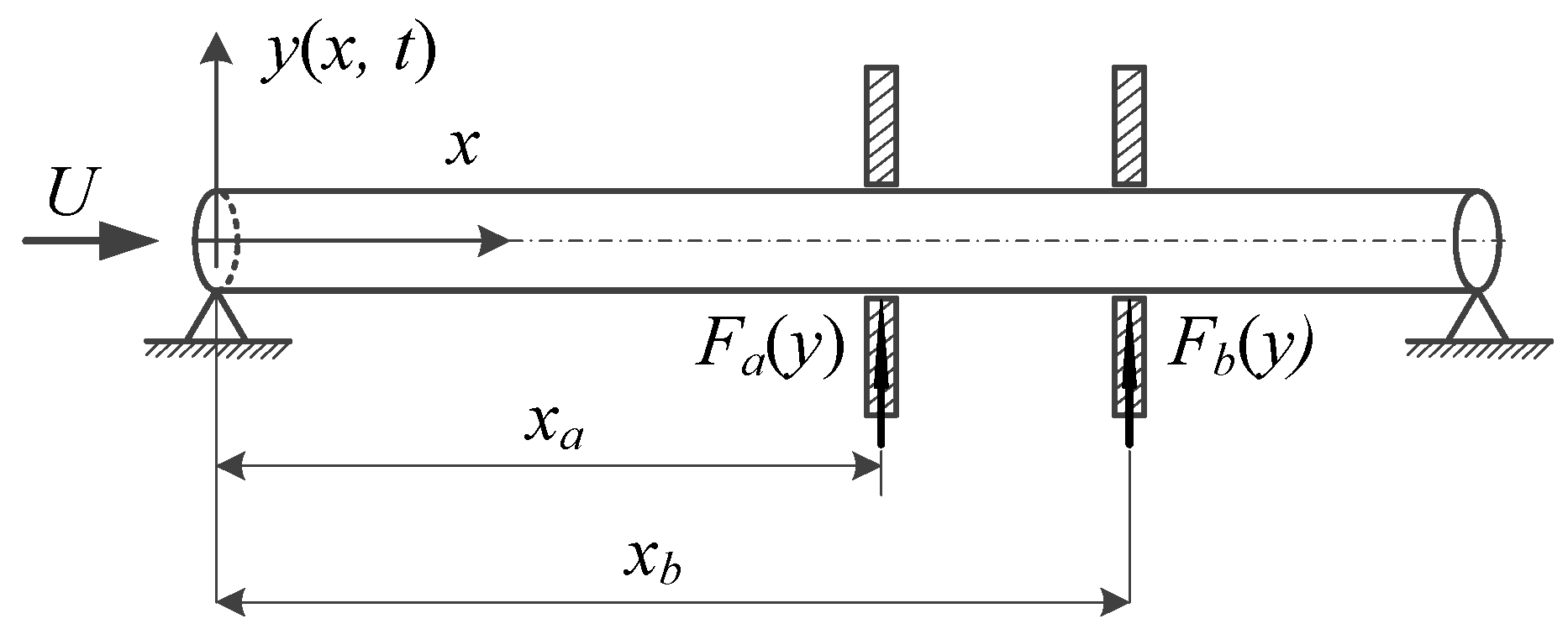
2.1. The Equation of Motion

A dynamic model for a drill string system, conveying pulsating fluid on a simply supported pipe, is developed in this section. The equations of motion, without taking into account the effect of motion constraints, are provided in [34,35,36]. As shown in Figure 1, based on the motion equation, considering the effect of support constraints [37], the cubic nonlinear spring forces F_a(y) and F_b(y) are used to simulate the reaction force [38], and the fluid–structure coupling motion differential equation of the drill string system is obtained, as follows:

$$\begin{array}{l}(m_{\mathrm{f}}+m_{\mathrm{d}})\frac{{\partial }^{2}y}{\partial t^2}+2m_{\mathrm{f}}U\frac{{\partial }^{2}y}{\partial x\partial t}+\left(1+a\frac{\partial }{\partial t}\right)EI\frac{{\partial }^{4}y}{\partial x^4}+\\ \left[m_{\mathrm{f}}{U}^2+m_{\mathrm{f}}\frac{\partial U}{\partial t}(l-x)-\left(1+a\frac{\partial }{\partial t}\right)\frac{E{A}_{\mathrm{p}}}{2I}{\int }_0^1{\left(\frac{\partial y}{\partial x}\right)}^{2}dx\right]\frac{{\partial }^{2}y}{\partial x^2}\\ +F_{\mathrm{a}}\left(y\right)\delta (x-x_{\mathrm{a}})+F_{\mathrm{b}}\left(y\right)\delta (x-x_{\mathrm{b}})=0\end{array}$$

(1)

where m_f represents the fluid mass per unit length, m_d is the mass of the drill string per unit length, U is the velocity of the fluid in the drill string, E is Young’s modulus, A is the cross-sectional area of the drill string and δ(x−x₀) is the Dirac delta function. Furthermore, l is the length of the drill string and I denotes the movement in the cross-sectional area. a is the viscoelastic damping coefficient, x_a and x_b represent the coordinates along the centerline of the drill string, K_a and K_b represent the support stiffness and y(x,t) is the lateral vibration displacement function of position x and time t. F_a(y) and F_b(y) represent the effects of the motion constraints on the drill string.

$$F_{\mathrm{a}}\left(y\right)=K_{\mathrm{a}}{y}^3$$

(2)

$$F_{\mathrm{b}}\left(y\right)=K_{\mathrm{b}}{y}^3$$

(3)

Furthermore, several dimensionless parameters can be defined as follows:

$$\begin{gathered} k_{\mathrm{a}}=\frac{K_{\mathrm{a}}{l}^5}{EI},\tau ={\left(\frac{EI}{m_{\mathrm{f}}+m_{\mathrm{d}}}\right)}^{\raisebox{1ex}{$1$}\!\left/ \!\raisebox{-1ex}{$2$}\right.}\frac{t}{l^2},u={\left(\frac{m_{\mathrm{f}}}{EI}\right)}^{\raisebox{1ex}{$1$}\!\left/ \!\raisebox{-1ex}{$2$}\right.}Ul,\beta =\frac{m_{\mathrm{f}}}{m_{\mathrm{f}}+m_{\mathrm{d}}},\kappa =\frac{A{l}^2}{2I}{k}_{\mathrm{b}}=\frac{K_{\mathrm{b}}{l}^5}{EI}, \\ \xi =\frac{x}{l},\eta =\frac{y}{l},\alpha ={\left(\frac{EI}{m_{\mathrm{f}}+m_{\mathrm{d}}}\right)}^{\raisebox{1ex}{$1$}\!\left/ \!\raisebox{-1ex}{$2$}\right.}\frac{a}{l^2},{\xi }_{\mathrm{a}}=\frac{x_{\mathrm{a}}}{l},{\xi }_{\mathrm{b}}=\frac{x_{\mathrm{b}}}{l} \end{gathered}$$

(4)

Substituting Equation (4) into Equation (1), the dimensionless equation form of non-linear dynamics can be rewritten as:

$$\begin{array}{l}\alpha \frac{{\partial }^5\eta }{\partial {\xi }^4\partial \tau }+\frac{{\partial }^4\eta }{\partial {\xi }^4}+\left[u^2+{\beta }^{\frac{1}{2}}\frac{\partial u}{\partial \tau }\left(1-\xi \right)\right]\frac{{\partial }^2\eta }{\partial {\xi }^2}+2{\beta }^{\frac{1}{2}}u\frac{{\partial }^2\eta }{\partial \xi \partial \tau }\\ +\frac{{\partial }^2\eta }{\partial {\tau }^2}-\kappa \frac{{\partial }^2\eta }{\partial {\xi }^2}{{\int }_0^1\left(\frac{\partial \eta }{\partial \xi }\right)}^{2}d\xi -2\alpha \kappa \frac{{\partial }^2\eta }{\partial {\xi }^2}{\int }_0^1\frac{\partial \eta }{\partial \xi }\frac{{\partial }^2\eta }{\partial \xi \partial \tau }d\xi \\ +k_{\mathrm{a}}{\eta }^3\delta \left(\xi -{\xi }_{\mathrm{a}}\right)+k_{\mathrm{b}}{\eta }^3\delta \left(\xi -{\xi }_{\mathrm{b}}\right)=0\end{array}$$

(5)

Moreover, assuming that the flow of fluid through the drill string is sinusoidal,

$$u=u_0\left(1+\mu \sin \omega \tau \right)$$

(6)

where ω is the forcing frequency, u₀ is the flow velocity, and μ is the perturbation amplitude.

2.2. Discretization of the System Model

In this study, the dynamic model is discretized by Galerkin’s method, and the vibration displacement η(ξ, τ) of the drill string can be expressed as:

$$\eta \left(\xi ,\tau \right)={\displaystyle \sum _{r=1}^N{\varphi }_r}\left(\xi \right)q_r\left(\tau \right)$$

(7)

where ${\varphi }_r$(ξ) is the appropriate set of base functions, q_r(τ) represents the corresponding generalized coordinates, and N is the total number of models used for the beam consideration. Substituting Equation (7) into Equation (5), multiplying by $\varphi$_I(ξ) and integrating throughout [0, 1], the dimensionless non-linear vibration equation of the drill string system is obtained:

$$\ddot{\mathit{q}}+\mathit{C}\dot{\mathit{q}}+\mathit{K}\mathit{q}+\mathit{f}\left(\mathit{q}\right)+\mathit{h}\left(\mathit{q},\dot{\mathit{q}}\right)=0$$

(8)

where C represents stationary damping and K represents stiffness matrices. It can be seen from reference [39] that N = 2 can obtain a higher calculation accuracy. The elements of C, K, f and h are composed of:

$$\begin{gathered} C_{ij}=C_{ij}{}^{\prime }+\left(2\sqrt{\beta }\mu u_0\sin \omega \tau \right)b_{ij}, \\ {K}_{ij}=K_{ij}{}^{\prime }+u_0^2\left(2\mu \sin \omega \tau +{\mu }^2{\sin }^2\omega \tau \right)c_{ij}+\left(\sqrt{\beta }\mu u_0\omega \cos \omega \tau \right)\left(c_{ij}-d_{ij}\right), \\ {f}_i=k_{\mathrm{a}}{\left[{\displaystyle \sum _{r=1}^N{\varphi }_r\left({\xi }_{\mathrm{a}}\right)q_r}\right]}^3{\varphi }_i\left({\xi }_{\mathrm{a}}\right)+k_{\mathrm{b}}{\left[{\displaystyle \sum _{r=1}^N{\varphi }_r\left({\xi }_{\mathrm{b}}\right)q_r}\right]}^3{\varphi }_i\left({\xi }_{\mathrm{b}}\right), \\ \begin{array}{l}\left(\begin{array}{l}{h}_1\\ h_2\end{array}\right)=2\alpha \kappa \left(q_1{q}_2\right)\left(\begin{array}{ll}{a}_{11}& \\ & a_{22}\end{array}\right)\left(\begin{array}{l}{\dot{q}}_1\\ {\dot{q}}_2\end{array}\right)\left(\begin{array}{ll}{a}_{11}& \\ & a_{22}\end{array}\right)\left(\begin{array}{l}{q}_1\\ q_2\end{array}\right)\\ +\kappa \left(q_1{q}_2\right)\left(\begin{array}{ll}{a}_{11}& \\ & a_{22}\end{array}\right)\left(\begin{array}{l}{q}_1\\ q_2\end{array}\right)\left(\begin{array}{ll}{a}_{11}& \\ & a_{22}\end{array}\right)\left(\begin{array}{l}{q}_1\\ q_2\end{array}\right)\end{array} \end{gathered}$$

(9)

where

$$C_{ij}{}^{\prime }=\alpha {\lambda }_j^4{\delta }_{ij}+2\sqrt{\beta }{u}_0{b}_{ij},K_{ij}{}^{\prime }={\lambda }_j^4{\delta }_{ij}+u_0^2{c}_{ij}$$

(10)

Furthermore, some constants are defined as follows:

$$\begin{gathered} a_{11}=-{\mathsf{\pi }}^2,a_{22}=-4{\mathsf{\pi }}^2,b_{ij}=\left\{\begin{array}{ll}\frac{2{\lambda }_i{\lambda }_j}{\left({\lambda }_j^2-{\lambda }_i^2\right)}\left[{\left(-1\right)}^{i+j}-1\right],& i\ne j\\ 0,& i=j\end{array}\right\} \\ {c}_{ij}=\left\{\begin{array}{ll}0,& i\ne j\\ -{\lambda }_i^2,& i=j\end{array}\right\},d_{ij}=\left\{\begin{array}{ll}\frac{4{\lambda }_i{\lambda }_j^3}{{\left({\lambda }_j^2-{\lambda }_i^2\right)}^2}\left[1-{\left(-1\right)}^{i+j}\right],& i\ne j\\ \raisebox{1ex}{$c_{jj}$}\!\left/ \!\raisebox{-1ex}{$2$}\right.,& i=j\end{array}\right\} \end{gathered}$$

(11)

For the purpose of numerical simulations, the state vector is introduced as follows:

$$\begin{gathered} \mathit{z}=\left\{q_1,q_2,{\dot{q}}_1,{\dot{q}}_2\right\} \\ \dot{\mathit{z}}=\mathit{A}\mathit{z}+\mu \left(\omega \cos \omega \tau {\mathit{B}}_1+\sin \omega \tau {\mathit{B}}_2\right)\mathit{z}+{\mu }^2{\sin }^2\omega \tau \left[{\mathit{B}}_3\right]\mathit{z}+\mathit{G}\left(\mathit{z}\right)+\mathit{Q}\left(\mathit{z}\right) \end{gathered}$$

(12)

where

$$\begin{array}{l}\mathit{A}=\left[\begin{array}{l}0I\\ -{K^{\prime }}_{ij}-{C^{\prime }}_{ij}\end{array}\right],{\mathit{B}}_1=\left[\begin{array}{cc}0& 0\\ -u_0\sqrt{\beta }\left(c_{ij}-d_{ij}\right)& 0\end{array}\right],{\mathit{B}}_2=\left[\begin{array}{cc}0& 0\\ -2u_0^2{c}_{ij}& -2\sqrt{\beta }{u}_0{b}_{ij}\end{array}\right]\\ {\mathit{B}}_3=\left[\begin{array}{cc}0& 0\\ -u_0^2{c}_{ij}& 0\end{array}\right],\mathit{G}={\left\{00-f_1-f_2\right\}}^{\mathrm{T}},Q={\left\{00-h_1-h_2\right\}}^{\mathrm{T}}\end{array}$$

(13)

3. Results and Discussion

The dynamic equations of the drill string system are described above. In the following sections, a series of parametric studies are investigated, namely forcing frequency ω, perturbation amplitude μ, mass ratio β and flow velocity u₀. Bifurcation diagrams and waveforms, phase diagrams and Poincaré maps are plotted and examined. The geometrical and physical parameters of the system drill string are shown in

Table 1. Main parameters of the drill string system.

Item	Notation	Value
Density of cutting fluid Density of drilling shaft	ρf ρz	8.65 × 102 kg/m3 7.8 × 103 kg/m3
Young’s modulus	E	2.14 × 1011 Pa
Internal diameter External diameter	d1 d2	7.68 × 10−2 m 1.27 × 10−2 m

, and the schematic diagram of the simulation condition is shown in Figure 2.

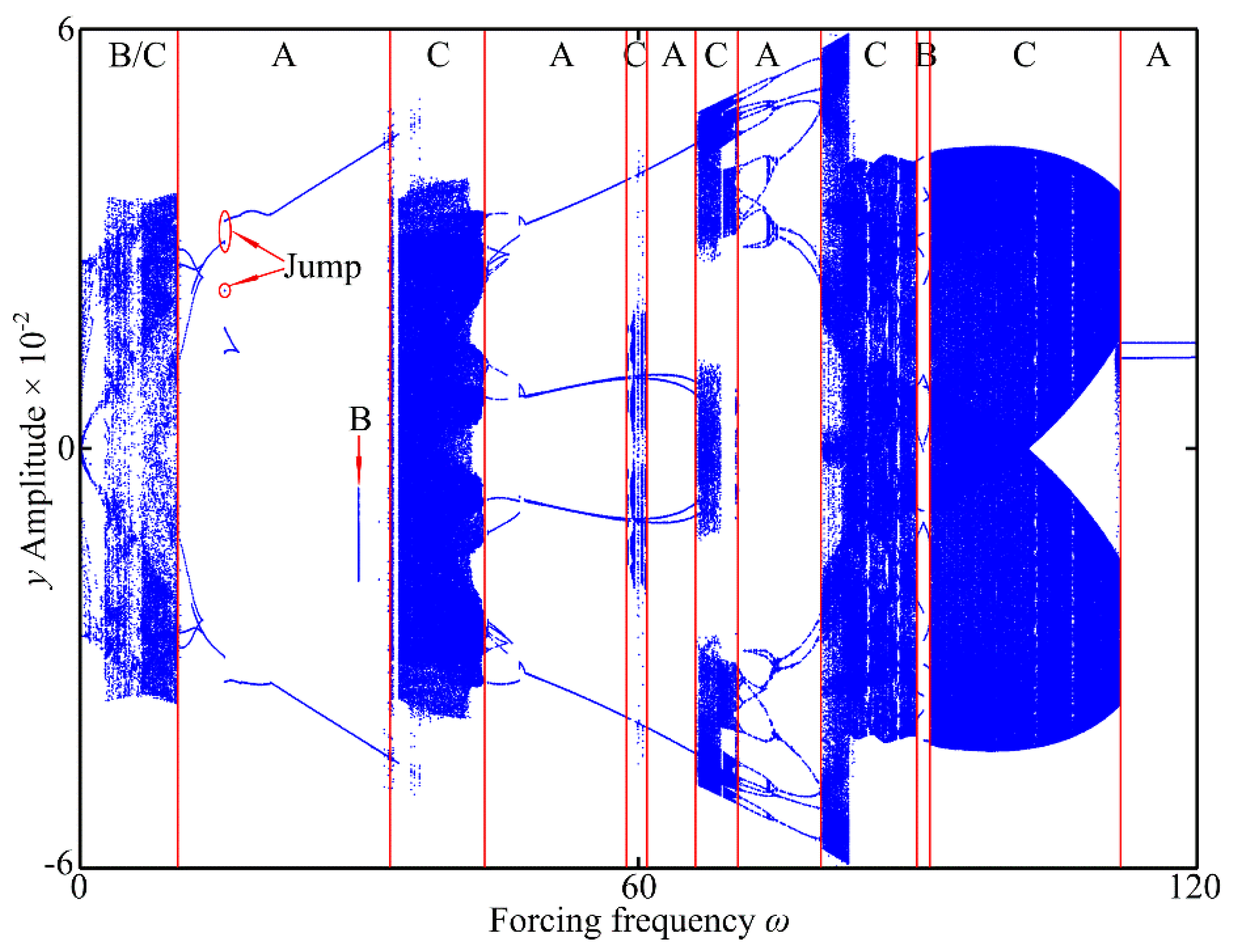
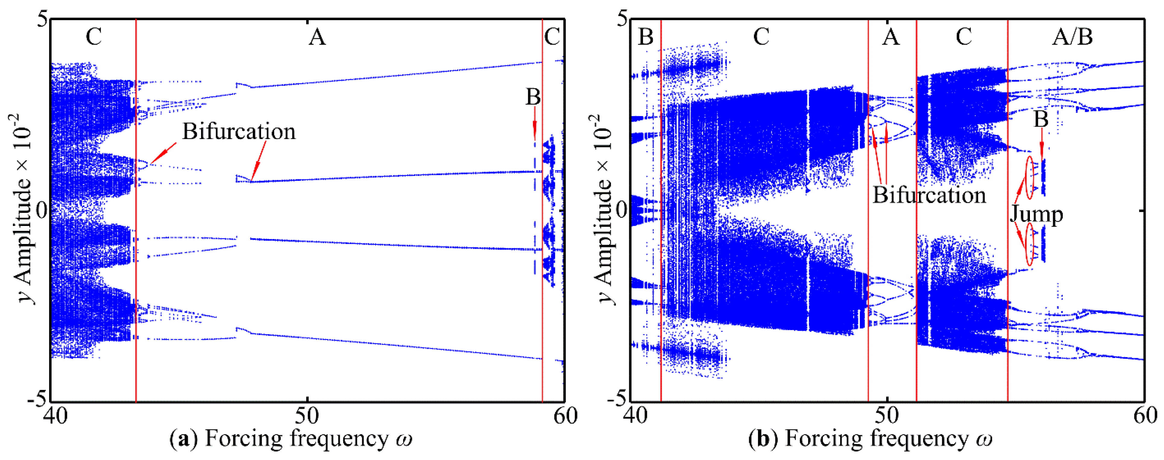
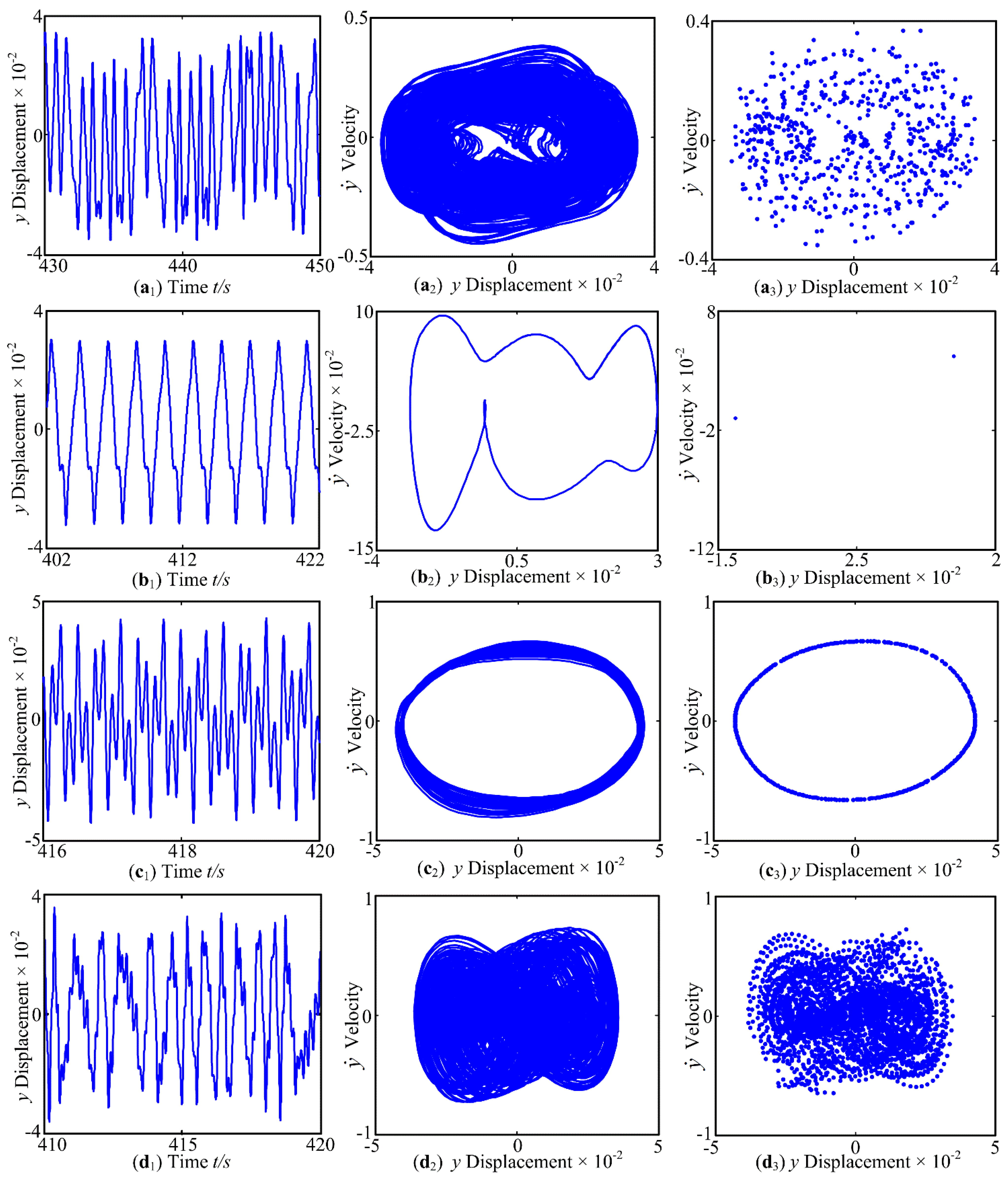
3.1. The Effect of Forcing Frequency ω on Dynamic Characteristics

The forcing frequency ω has a significant effect on the dynamic response of the drill string system. In order to investigate the forcing frequency of the drill string system in detail, all parameters except the forcing frequency are taken as constants. The corresponding bifurcation diagram is shown in Figure 3, with ω as the control parameter in the interval [0, 120] at k_a = 0 and k_b = 0. Figure 4 shows the bifurcation diagram of forced frequency ω when k_a = k_b = 0, k_a = 2.8 × 10⁵ and k_b = 2 × 10³ in the range of [40, 60] respectively. In the bifurcation diagram, the abscissa is the forcing frequency, and the ordinate is the displacement amplitude of the vibration at the center of the drill string. As shown in Figure 3, quasi-periodic and chaotic motions can be observed in the range of [0, 10.55], when ω = 8, the corresponding dynamic response of the system is shown in Figure 5(a₁–a₃). It can be observed that the system shows chaotic characteristics, the Poincaré map appears scattered points. As the forcing frequency is increased, namely 10.55 < ω < 33.1, a series of inverse period-doubling bifurcations appears in the system, where the system exists periodic-6, periodic-2 motion and apparent jump discontinuity.

The related periodic-2 motion at ω = 21 is shown in Figure 5(b₁–b₃) with waveform, phase diagram and Poincaré map, which indicates that the system experiences periodic-2 motion and only two points are shown in the Poincaré map. Figure 5(c₁–c₃) show the dynamic characteristics of the system at ω = 29.9, The Poincaré map is a closed circle, and the system features quasi-periodic motion. To further analyze the dynamics of the drill string system, the local bifurcation diagram of the forcing frequency ω in the range of [40, 60] is given in Figure 4a. As the forcing frequency is increased, the chaotic responses are observed in the interval [33.1, 43.5]. The related chaotic motion at ω = 35 is shown in Figure 5(d₁–d₃) by a waveform, phase diagram and Poincaré map. By increasing ω from 43.5 to 57.75, a series of inverse period-doubling bifurcations appears in the system, and the system response presents the phenomenon of period-doubling reverse bifurcation, the period number of vibration changes exponentially, and the chaotic motion of the system is transformed into periodic motion in the form of period-doubling reverse bifurcation.

Figure 5(e₁–e₃) presents the periodic-8 motion, which is due to the presence of eight points in the Poincaré map at ω = 46.35. When the increased excitation frequency is ω = 47.5, as shown in Figure 5(f₁–f₃), the system motion state is periodic-4 motion, and four points exhibit in the Poincaré map. With the increase in ω, the system shows chaotic intermittency motion at [57.75, 60.75] in Figure 3. Figure 5(g₁–g₃) shows the dynamic response of the system when ω = 59.5, the observation shows that the system is in chaotic motion. Further increasing the forcing frequency ω, the system displays strong non-linear characteristics, the vibration amplitude significantly increases and periodic motion, quasi-periodic motion and chaotic motion appear at [66.25, 120]. The system again displays the phenomenon of period-doubling reverse bifurcation in the range of [70.55, 79.75]. In the range [89.5, 91.25], a narrow quasi-periodic motion is observed, as shown in Figure 5(h₃), and two closed circles are exhibited in the Poincaré map. The dynamic characteristics of the system at ω = 110 are displayed in Figure 5(i₁–i₃). It can be found that the system has obvious chaotic characteristics. Figure 5(j₁–j₃) presents the periodic-2 motion at ω = 119 via waveform, phase diagram and Poincaré map.

Figure 4b presents the bifurcation diagram of the forcing frequency ω at k_a = 2.8 × 10⁵ and k_b = 2 × 10³ in the range [40, 60]. In the interval [40, 41.22], the dynamic response of the system mostly comprises quasi-periodic motion. With the increase in the forcing frequency from 41.22 to 54.68, the system changes from chaotic motion at [41.22, 49.26], through to a series of inverse period-doubling bifurcations at 49.26 < ω < 51.16, to return to chaotic motion at [51.16, 54.68]. As the forcing frequency continues to increase, the system exhibits periodic motion, quasi-periodic motion at 51.16 < ω < 60 and obvious jump discontinuity. It is observed that the system has abundant dynamic behaviors—periodic, quasi-periodic and chaotic behaviors all alternating with each other with different support stiffness—and the system shows complicated non-linear phenomena, and the exchange frequency between the motion is enhanced.

3.2. The Effect of Perturbation Amplitude μ on Dynamic Characteristics

Under different support stiffness conditions, the influence of the perturbation amplitude μ on the dynamics characteristics of the system is analyzed. The corresponding bifurcation diagrams, with μ as the control parameter at [0.2, 0.6], are shown in Figure 6. The response of the drill string system at k_a = 3.1 × 10⁶ and k_b = 0 is demonstrated in detail in Figure 6a. The system shows chaotic characteristics at [0.2, 0.5225], and the intensity of chaotic motion is increased. Figure 7(a₁–a₃) shows the waveform, phase diagram and Poincaré map of the system at μ = 0.426, at which point the system has chaotic motion. With the increasing perturbation amplitude μ, the system shows periodic motion and quasi-periodic motion. The jump discontinuous non-linear phenomenon appears at (0.5225, 0.5745), and the system dynamic response is shown in Figure 7(b₁–b₃) at μ = 0.571. As can be seen in this figure, the system exhibits quasi-periodic motion. With the further increase in the perturbation amplitude, the motion of the system is a narrow period-2 at [0.5475, 0.5805]. As shown in Figure 7(c₁–c₃), period-2 motion is observed at μ = 0.576.

Increasing the perturbation amplitude from 0.5805 to 0.6, the system returns to chaotic motion.

Figure 6b presents the system bifurcation diagram with ω in the range of [0.2, 0.6] at k_a = 2.6 × 10⁶, k_b = 8.6 × 10⁶. In the interval [0.2, 0.258], the system shows the non-linear characteristics of periodic, quasi-periodic and chaotic motion. As μ is further increased, it can be observed that the system exhibits periodic-4 motions, periodic-2 motions, periodic-10 motions, jump discontinuity phenomenon and period-doubling bifurcations phenomenon in the interval (0.258, 0.519). With the further increase in the perturbation amplitude, the system markedly exhibits chaotic motion at [0.519, 0.6]. Compared with Figure 6a, it can be seen that the chaotic motion region of the system can be reduced, to a certain extent, by adjusting the combination of support stiffness coefficients. This is mainly because the change in support stiffness causes the change in the inherent characteristics of the system. It can be seen that the support stiffness has a complex impact on the non-linear dynamic behavior of the system.

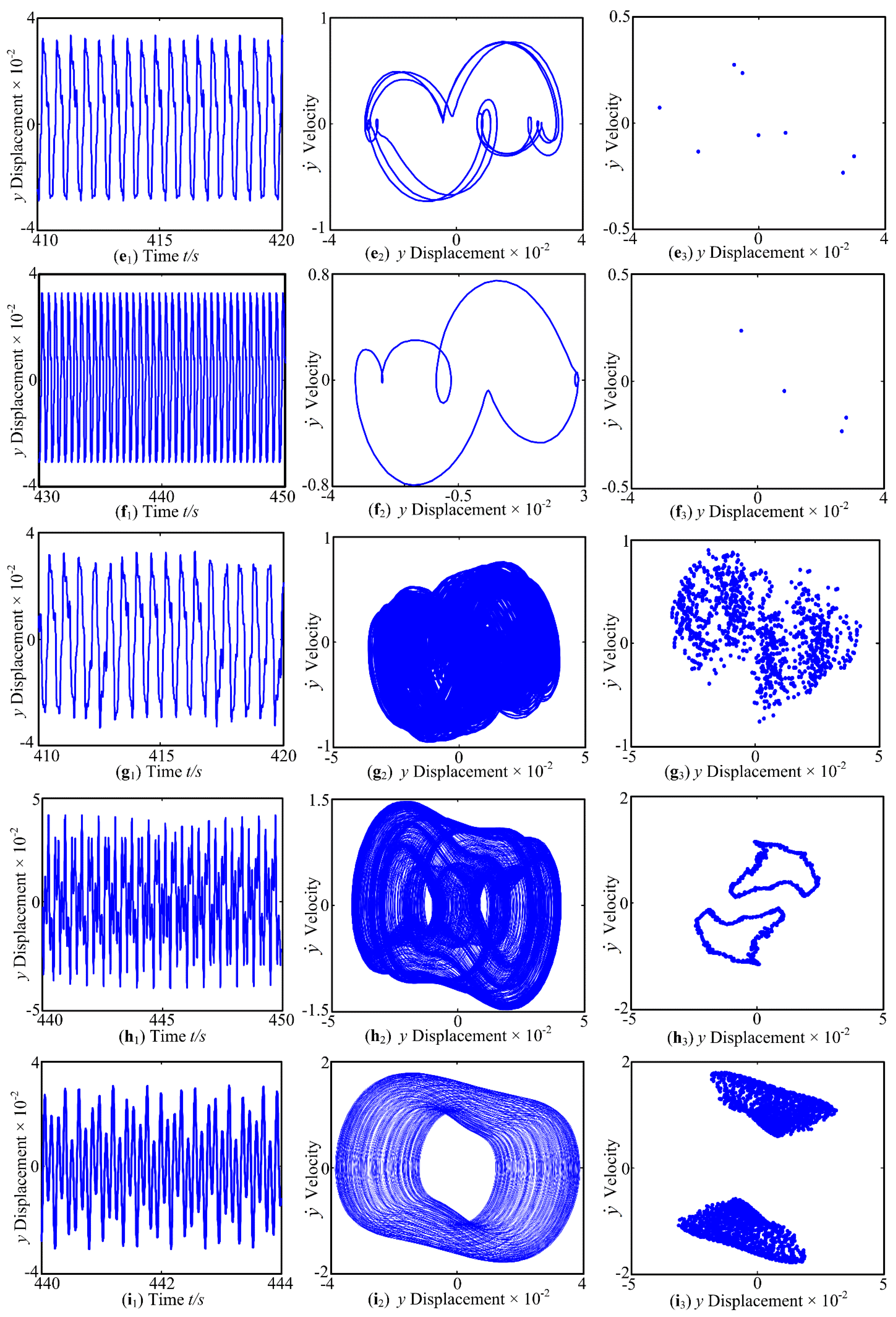
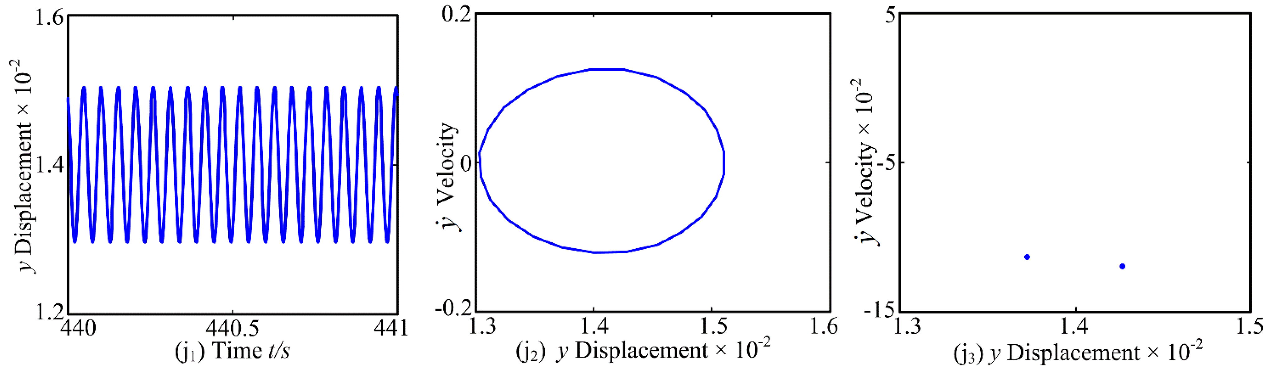
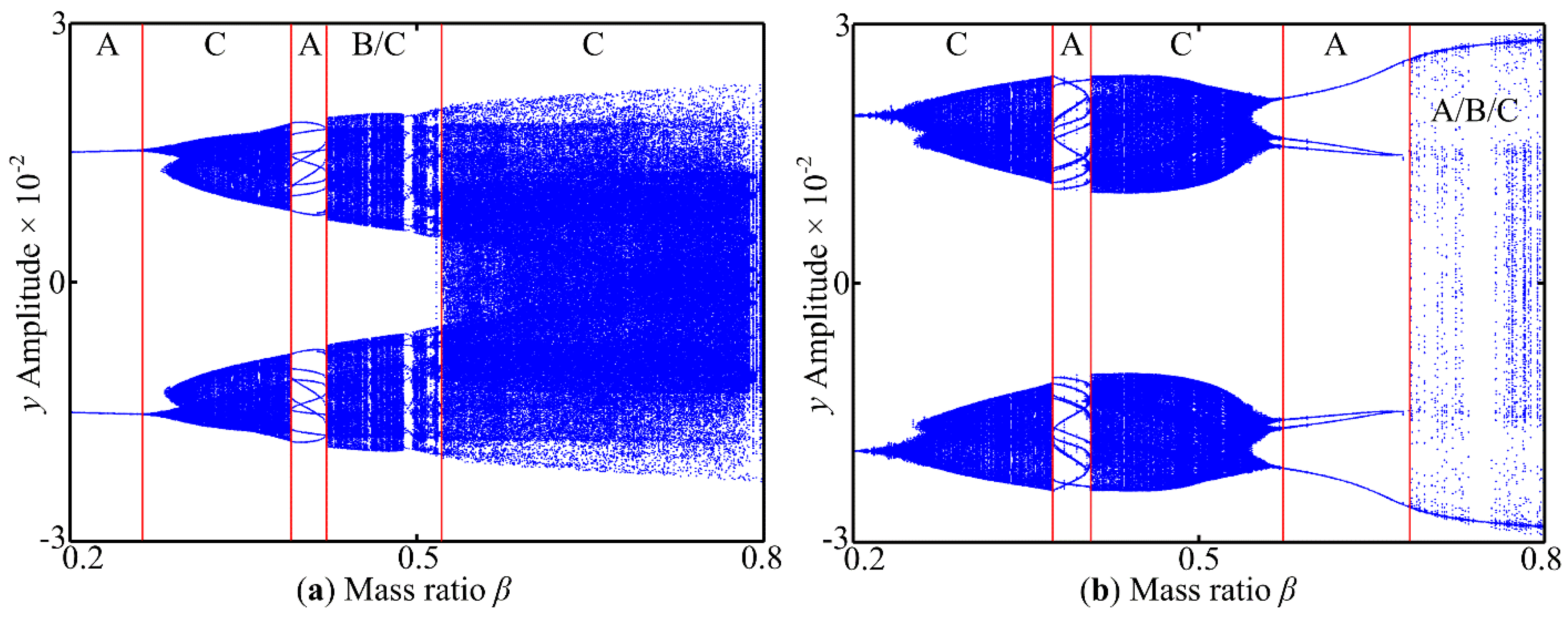
3.3. The Effect of Mass Ratio β on Dynamic Characteristics

Because of the different fluid masses, mass ratio β is a key parameter in evaluating the system vibration characteristics. The drill string mass ratio is taken as the control parameter to carry out a detailed study. Figure 8a displays the bifurcation diagram in the interval [0.2, 0.8] at k_a = 2.1 × 10⁶ and k_b = 8.6 × 10⁴. The system is in periodic motion at [0.2, 0.262], as shown in Figure 9(a₁–a₃) at β = 0.218, the system presents periodic-2 motion by the waveform, phase diagram and Poincaré map. With the increase in the mass ratio from 0.262 to 0.39, the response of the system is chaotic motion, and the chaotic motion region gradually increases. Further increase in the mass ratio, the motion becomes periodic in the interval [0.39, 0.422]. For the mass ratio from 0.422 to 0.523, the system alternates between exhibiting quasi-periodic motion and chaotic motion. Figure 9(b₁–b₃) shows the vibration response of the system at the mass ratio β = 0.521, the system is quasi-periodic motion. As the mass ratio β continues to increase, the system exhibits chaotic motion at [0.523, 0.8], and the chaotic motion area significantly increases. The dynamic responses at β = 0.752 are presented in Figure 9(c₁–c₃), and the system exhibits chaotic motion.

Figure 8b displays the bifurcation diagram at k_a = 9.2 × 10⁵ and k_b = 8.6 × 10⁵, with the mass ratio β as the control parameter in the range [0.2, 0.8]. When the mass ratio increases, the system presents chaotic characteristics at [0.2, 0.373], after periodic motion from 0.373 to 0.406, at which point the system returns to chaotic motion. At [0.572, 0.682], periodic-6 motion is observed. By further increasing β, the system response consists of periodic, quasi-periodic and chaotic behaviors. Compared with Figure 8a, the chaotic area is reduced, the intensity of chaotic motion decreases, and the area of periodic motion increases.

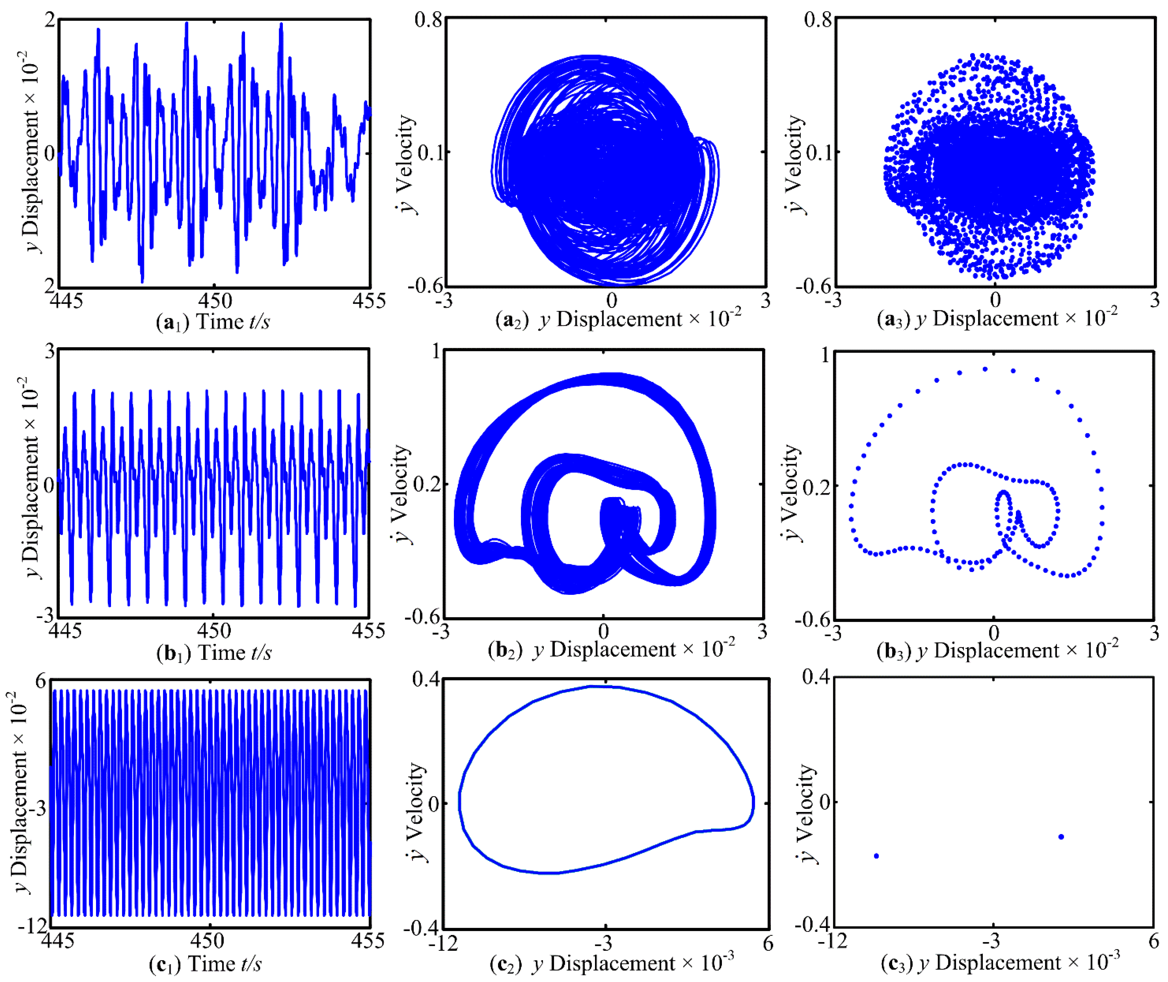
3.4. The Effect of Flow Velocity u₀ on Dynamic Characteristics

This section studies the effect of flow velocity u₀ on the dynamic behavior of the drill string system. The corresponding bifurcation diagram of the system with flow velocity under support stiffness k_a = 2.6 × 10⁶ and k_b = 0 is shown in Figure 10a. For the flow velocity in the range of [1.5, 2.852], the periodic-1 motion is observed. With the increase in the flow velocity from 2.852 to 3.986, the system exhibits quasi-periodic motion and chaotic motion. Figure 11(a₁–a₃) presents quasi-periodic motion at u₀ = 3.384 of the system. As the flow velocity further increases, the system presents narrow periodic motion at [3.986, 4.054]. Periodic motion is observed at u₀ = 4.018 in Figure 11(b₁–b₃). With increasing u₀ from 4.054 to 4.5, a large amplitude chaotic response is observed. Figure 11(c₁–c₃) show the relevant vibration response of the system at u₀ = 4.386, and the motion state exhibits chaotic behavior.

Figure 10b displays the bifurcation diagram at k_a = 0 and k_b = 0, with flow velocity u₀ as the control parameter in the range [1.5, 4.5]. It is found that the system exhibits period-1 motion at the intervals [1.5, 2.912]. With the gradual increase in the flow velocity from 2.912 to 3.622, the system exhibits quasi-periodic motion and chaotic behavior, and it is found that the chaotic region gradually increases. With the flow velocity continuing to increase, the system evolves into short period-2 motion in the range [3.622, 3.678], after which the system goes back to a chaotic behavior from 3.678 to 3.928. With the flow velocity increasing even further, the system evolves into short narrow periodic-3 motion and then enters periodic-2 motion with obvious jump discontinuity in the range [3.928, 4.5]. Compared with Figure 10a, it can be seen that, as the vibration amplitude of the system increases, the chaotic motion region decreases, and the periodic motion region significantly increases. The support stiffness has a complex effect on the inherent characteristics of the drill string system dynamics.

4. Conclusions

The non-linear dynamic characteristics of a fluid-structure coupled drilling system are studied in this paper. The effects of forcing frequency ω, perturbation amplitude μ, mass ratio β and flow velocity u₀ on the dynamic characteristics are investigated. The research in this paper seeks not only to understand the dynamic response of the drill string, but also provides some references for vibration control and the optimization of vibration systems. The research conclusions are listed as follows:

(1)

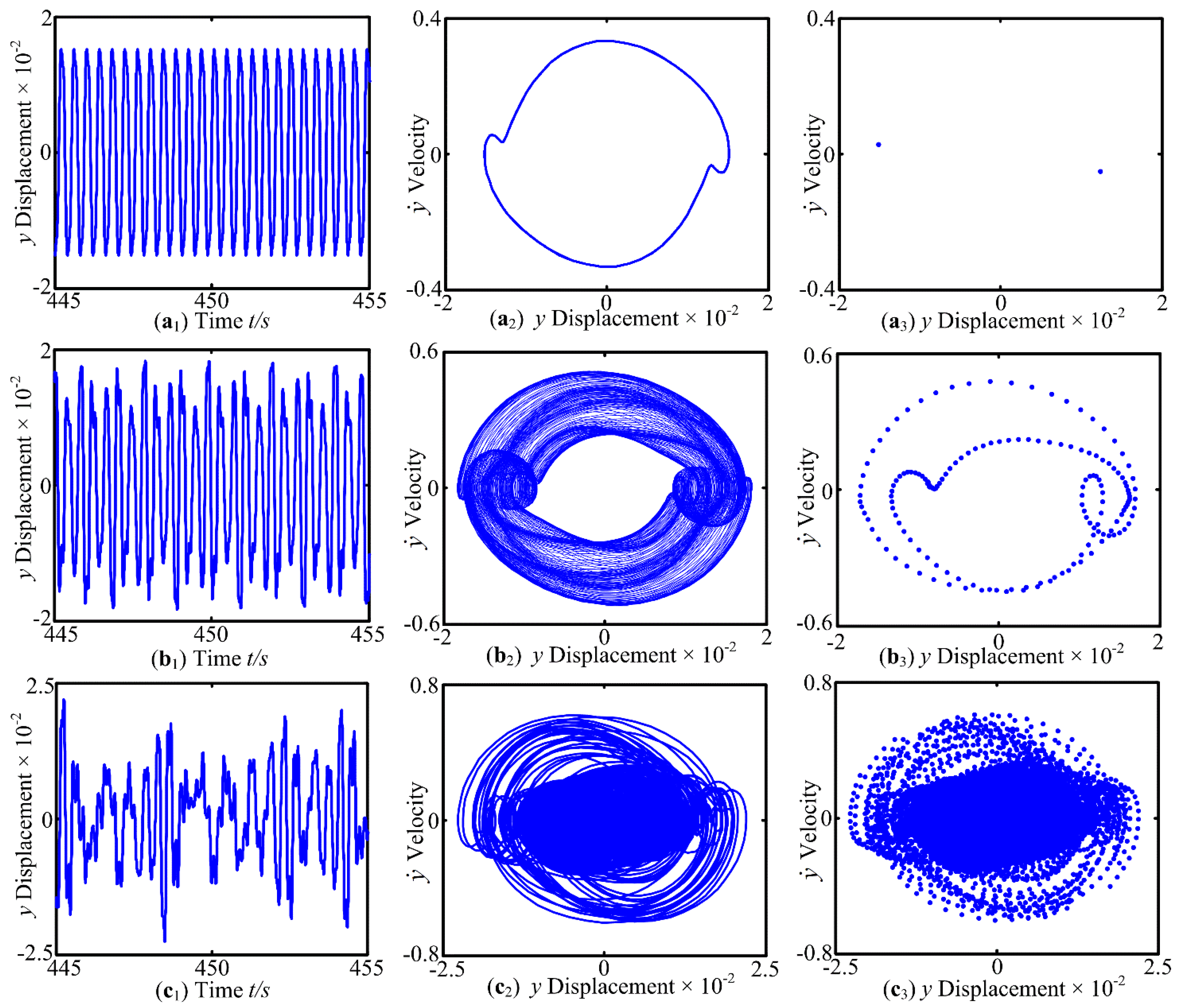
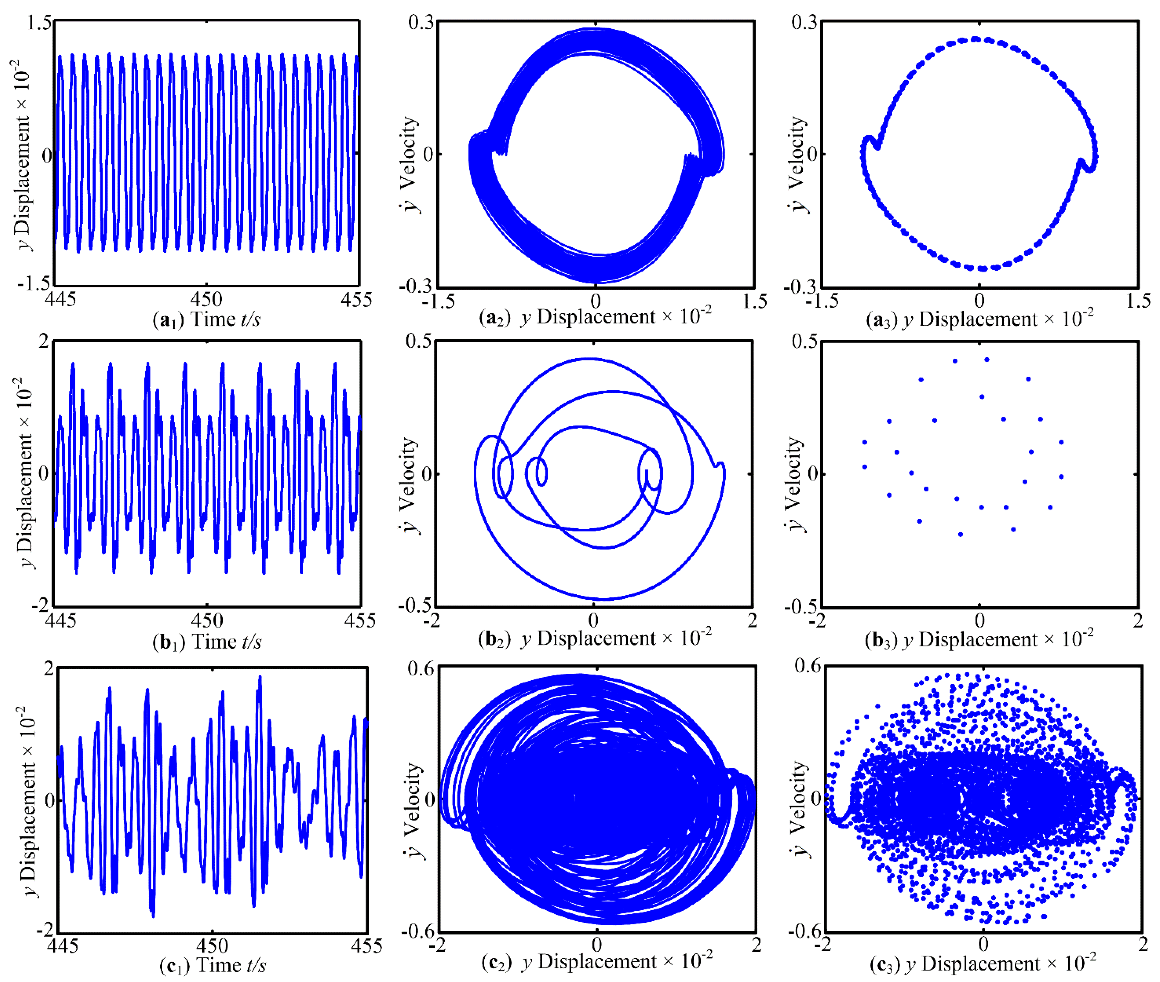
Under the control parameter of forcing frequency ω, the vibration system exhibits periodic motion, quasi-periodic motion and chaotic behavior, and the phenomenon of jumping discontinuity appears. In addition, a period-doubling reverse bifurcation from chaotic motion to periodic motion is exhibited. The support stiffness causes a change in the inherent characteristics, which has an impact on the dynamic of the system.

(2)

With the increase in the perturbation amplitude μ, the periodic motion, quasi-periodic motion, chaotic behavior, jump discontinuity phenomenon and period-doubling bifurcations phenomenon of the system are transformed. In addition, under certain combinations of supporting stiffness, the region of chaotic motion becomes smaller and the area of periodic motion grows. The support stiffness can, to a certain extent, cause a change of the inherent characteristics of the system.

(3)

As mentioned above, with the increase in the mass ratio β and flow velocity u₀, the intensity of chaotic motion increases, and the system exhibits periodic and quasi-periodic responses and chaotic motion. Moreover, under certain combinations of supporting stiffness, periodic motion increases and the chaotic region shrinks.

References

1. Ghasemloonia, A.; Rideout, D.G.; Butt, S.D. A review of drillstring vibration modeling and suppression methods. J. Pet. Sci. Eng. 2015, 131, 150–164. [Google Scholar] [CrossRef]
2. Liu, Y.; Joseph, P.C.; Sa, R.D. Numerical and experimental studies of stick–slip oscillationsin drill-strings. Nonlinear Dyn. 2017, 90, 2959–2978. [Google Scholar] [CrossRef] [Green Version]
3. Real, F.F.; Batou, A.; Ritto, T.G.; Desceliers, C.; Aguiar, R.R. Hysteretic bit/rock interaction model to analyze the torsional dynamics of a drill string. Mech. Syst. Signal Process. 2018, 111, 222–233. [Google Scholar] [CrossRef] [Green Version]
4. Kamel, J.M.; Yigit, A.S. Modeling and analysis of stick–slip and bit bounce in oil well drillstrings equipped with dragbits. J. Sound Vib. 2014, 333, 6885–6899. [Google Scholar] [CrossRef]
5. Liang, F.; Gao, A.; Yang, X.D. Dynamical analysis of spinning functionally graded pipes conveying fluid with multiple spans. Appl. Math. Model. 2020, 83, 454–469. [Google Scholar] [CrossRef]
6. Liang, F.; Yang, X.D.; Qian, Y.J.; Zhang, W. Transverse free vibration and stability analysis of spinning pipes conveying fluid. Int. J. Mech. Sci. 2018, 137, 195–204. [Google Scholar] [CrossRef]
7. Liang, F.; Yang, X.D.; Zhang, W.; Qian, Y.J. Dynamical modeling and free vibration analysis of spinning pipes conveying fluid with axial deployment. J. Sound Vib. 2018, 417, 65–79. [Google Scholar] [CrossRef]
8. Liang, F.; Yang, X.D.; Zhang, W.; Qian, Y.J. Vibrations in 3D space of a spinning supported pipe exposed to internal and external annular flows. J. Fluids Struct. 2019, 87, 247–262. [Google Scholar] [CrossRef]
9. Guzek, A.; Shufrin, I.; Pasternak, E.; Dyskin, A. Influence of drilling mud rheology on the reduction of vertical vibrations in deep rotary drilling. J. Pet. Sci. Eng. 2015, 135, 375–383. [Google Scholar] [CrossRef]
10. Shen, H.; Padoussis, M.P.; Wen, J.; Yu, D.; Wen, X. The beam-mode stability of periodic functionally-graded-material shells conveying fluid. J. Sound Vib. 2014, 333, 2735–2749. [Google Scholar] [CrossRef]
11. Sheng, G.G.; Wang, X. Nonlinear response of fluid-conveying functionally graded cylindrical shells subjected to mechanical and thermal loading conditions. Compos. Struct. 2017, 168, 675–684. [Google Scholar] [CrossRef]
12. Zhou, X.W.; Dai, H.L.; Wang, L. Dynamics of axially functionally graded cantilevered pipes conveying fluid. Compos. Struct. 2018, 190, 112–118. [Google Scholar] [CrossRef]
13. An, C.; Su, J. Dynamic behavior of axially functionally graded pipes conveying fluid. Math. Probl. Eng. 2017, 2017, 6789634. [Google Scholar] [CrossRef] [Green Version]
14. Volpi, L.P.; Lobo, D.M.; Ritto, T.G. A stochastic analysis of the coupled lateral-torsional drill string vibration. Nonlinear Dyn. 2021, 103, 49–62. [Google Scholar] [CrossRef]
15. Zhu, K.; Chung, J. Nonlinear lateral vibrations of a deploying Euler–Bernoulli beam with a spinning motion. Int. J. Mech. Sci. 2015, 90, 200–212. [Google Scholar] [CrossRef]
16. Huo, Y.L.; Wang, Z.M. Dynamic analysis of a vertically deploying/retracting cantilevered pipe conveying fluid. J. Sound Vib. 2016, 360, 224–238. [Google Scholar] [CrossRef]
17. Vaziri, V.; Oladunjoye, I.O.; Kapitaniak, M.; Aphale, S.S.; Wierci, G.M. Parametric analysis of a sliding-mode controller to suppress drill-string stick-slip vibration. Meccanica 2020, 55, 2475–2492. [Google Scholar] [CrossRef]
18. Eftekhari, M.; Hosseini, M. On the stability of spinning functionally graded cantilevered pipes subjected to fluid-thermomechanical loading. Int. J. Struct. Stab. Dyn. 2016, 16, 1550062. [Google Scholar] [CrossRef]
19. Kapitaniak, M.; Hamaneh, V.V.; Chávez, J.P.; Nandakumar, K.; Wiercigroch, M. Unveiling complexity of drill-String vibrations: Experiments and modeling. Int. J. Mech. Sci. 2015, 101–102, 324–337. [Google Scholar] [CrossRef]
20. Gupta, S.K.; Wahi, P. Global axial-torsional dynamics during rotary drilling. J. Sound Vib. 2016, 375, 332–352. [Google Scholar] [CrossRef]
21. Lian, Z.; Qiang, Z.; Lin, T.; Wang, F. Experimental and numerical study of drill string dynamics in gas drilling of horizontal wells. J. Nat. Gas Sci. Eng. 2015, 27, 1412–1420. [Google Scholar] [CrossRef]
22. Boukredera, F.S.; Hadjadj, A.; Youcefi, M.R. Drilling vibrations diagnostic through drilling data analyses and visualization in real time application. Earth Sci. Inform. 2021, 7, 1–18. [Google Scholar]
23. Lenwoue, A.R.K.; Deng, J.; Feng, Y.; Li, H.; Oloruntoba, A.; Selabi, N.; Marembo, M.; Sun, Y. Numerical Investigation of the Influence of the Drill String Vibration Cyclic Loads on the Development of the Wellbore Natural Fracture. Energies 2021, 14, 2015. [Google Scholar] [CrossRef]
24. Moharrami, M.J.; Martins, C.; Shiri, H. Nonlinear integrated dynamic analysis of drill strings under stick-slip vibration. Appl. Ocean. Res. 2021, 108, 102521. [Google Scholar] [CrossRef]
25. Kapluno, V.J.; Khajiyeva, L.A.; Martyniuk, M.; Sergaliyev, A.S. On the dynamics of drilling. Int. J. Eng. Sci. 2020, 146, 103184. [Google Scholar] [CrossRef]
26. Liu, Y.; Lin, W.; Chávez, J.P.; Sa, R.D. Torsional stick-slip vibrations and multistability in drill-strings. Appl. Math. Model. 2019, 76, 545–557. [Google Scholar] [CrossRef]
27. Mfs, A.; Ed, B.; Nvdwa, B. Nonlinear dynamic modeling and analysis of borehole propagation for directional drilling. Int. J. Non-Linear Mech. 2019, 113, 178–201. [Google Scholar]
28. Salehi, M.M.; Moradi, H. Nonlinear multivariable modeling and stability analysis of vibrations in horizontal drill string. Appl. Math. Model. 2019, 71, 525–542. [Google Scholar] [CrossRef]
29. Zhang, H.; Di, Q.; Li, N.; Wang, W.; Chen, F. Measurement and simulation of nonlinear drillstring stick-slip and whirling vibrations. Int. J. Non-Linear Mech. 2020, 125, 103528. [Google Scholar] [CrossRef]
30. Xue, Q.; Leung, H.; Huang, L.; Zhang, R.; Liu, B.; Wang, J.; Li, L. Modeling of torsional oscillation of drillstring dynamics. Nonlinear Dyn. 2019, 96, 267–283. [Google Scholar] [CrossRef]
31. Xue, Q.; Leung, H.; Wang, R.; Liu, B.; Guo, S. The chaotic dynamics of drilling. Nonlinear Dyn. 2016, 83, 2013–2018. [Google Scholar] [CrossRef]
32. Lu, C.; Wu, M.; Chen, L.; Cao, W. An event-triggered approach to torsional vibration control of drill-string system using measurement-while-drilling data. Control. Eng. Pract. 2020, 106, 104668. [Google Scholar] [CrossRef]
33. Vromen, T.; Dai, C.H.; Nathan, V.; Oomen, T.; Astrid, P.; Doris, P. Mitigation of Torsional Vibrations in Drilling Systems: A Robust Control Approach. IEEE Trans. Control Syst. Technol. 2017, 27, 249–265. [Google Scholar] [CrossRef]
34. Panda, L.N.; Kar, R.C. Non-linear dynamics of a pipe conveying pulsating fluid with parametric and internal resonances. Nonlinear Dyn. 2007, 49, 9–30. [Google Scholar] [CrossRef]
35. Panda, L.N.; Kar, R.C. Non-linear dynamics of a pipe conveying pulsating fluid with combination, principal parametric and internal resonances. J. Sound Vib. 2008, 309, 375–406. [Google Scholar] [CrossRef]
36. Jin, J.D.; Song, Z.Y. Parametric resonances of supported pipes conveying pulsating fluid. J. Fluids Struct. 2005, 20, 763–783. [Google Scholar] [CrossRef]
37. Kapitaniak, M.; Vaziri, V.; Chávez, J.P.; Wiercigroch, M. Experimental studies of forward and backward whirls of drill-string. Mech. Syst. Signal Process. 2018, 100, 454–465. [Google Scholar] [CrossRef] [Green Version]
38. Wang, L. A further study on the non-linear dynamic of simply supported pipes conveying pulsating fluid. Int. J. Non-Linear Mech. 2009, 44, 115–121. [Google Scholar] [CrossRef]
39. Jin, J.D. Stability and chaotic motions of a restrained pipe conveying fluid. J. Sound Vib. 1997, 208, 427–439. [Google Scholar] [CrossRef]
Figure 1. Schematic diagram of a simply supported drill string with constraints.
Applsci 11 09047 g001
Figure 2. Simulation condition schematic.
Applsci 11 09047 g002
Figure 3. Bifurcation diagram of system response with ω, ka = kb = 0 (A: periodic motion; B: quasi-periodic motion; C: chaotic motion).
Applsci 11 09047 g003
Figure 4. Bifurcation diagram of system response with ω, (a) ka = kb = 0; (b) ka = 2.8 × 10⁵, kb = 2 × 10³ (A: periodic motion; B: quasi-periodic motion; C: chaotic motion).
Applsci 11 09047 g004
Figure 5. Waveform (1), phase diagram (2) and Poincaré map (3) with ω = 8 chaotic motion (a), ω = 21 Periodic-2 motion (b), ω = 29.9 quasi-periodic motion (c), ω = 35 chaotic motion (d), ω = 46.35 Periodic-8 motion (e), ω = 47.5 Periodic-4 motion (f), ω = 59.5 chaotic motion (g), ω = 89.5 quasi-periodic motion (h), ω = 110 chaotic motion (i) and ω = 119 Periodic-2 motion (j).
Applsci 11 09047 g005aApplsci 11 09047 g005bApplsci 11 09047 g005c
Figure 6. Bifurcation diagram of system response with μ: (a) ka = 3.1 × 10⁶, kb = 0; (b) ka = 2.6 × 10⁶, kb = 8.6 × 10⁶ (A: periodic motion; B: quasi-periodic motion; C: chaotic motion).
Applsci 11 09047 g006
Figure 7. Waveform (1), phase diagram (2) and Poincaré map (3) with μ = 0.426 chaotic motion (a), μ = 0.571 quasi-periodic motion (b) and μ = 0.576 periodic motion (c).
Applsci 11 09047 g007
Figure 8. Bifurcation diagram of system response with β: (a) ka = 2.1 × 10⁶, kb = 8.6 × 10⁴; (b) ka = 9.2 × 10⁵, kb = 8.6 × 10⁵ (A: periodic motion; B: quasi-periodic motion; C: chaotic motion).
Applsci 11 09047 g008
Figure 9. Waveform (1), phase diagram (2) and Poincaré map (3) with β = 0.218 Periodic-2 motion (a), β = 0.521 quasi-periodic motion (b) and β = 0.752 chaotic motion (c).
Applsci 11 09047 g009
Figure 10. Bifurcation diagram of system response with u0: (a) ka = 2.6 × 10⁶, kb = 0; (b) ka = kb = 0 (A: periodic motion; B: quasi-periodic motion; C: chaotic motion).
Applsci 11 09047 g010
Figure 11. Waveform (1), phase diagram (2) and Poincaré map (3) with u0 = 3.384 quasi-periodic motion (a), u0 = 4.018 periodic motion (b), u0 = 4.386 chaotic motion (c).
Applsci 11 09047 g011