A Randomized Bag-of-Birds Approach to Study Robustness of Automated Audio Based Bird Species Classification

Abstract

The automatic classification of bird sounds is an ongoing research topic, and several results have been reported for the classification of selected bird species. In this contribution, we use an artificial neural network fed with pre-computed sound features to study the robustness of bird sound classification. We investigate, in detail, if and how the classification results are dependent on the number of species and the selection of species in the subsets presented to the classifier. In more detail, a bag-of-birds approach is employed to randomly create balanced subsets of sounds from different species for repeated classification runs. The number of species present in each subset is varied between 10 and 300 by randomly drawing sounds of species from a dataset of 659 bird species taken from the Xeno-Canto database. We observed that the shallow artificial neural network trained on pre-computed sound features was able to classify the bird sounds. The quality of classifications were at least comparable to some previously reported results when the number of species allowed for a direct comparison. The classification performance is evaluated using several common measures, such as the precision, recall, accuracy, mean average precision, and area under the receiver operator characteristics curve. All of these measures indicate a decrease in classification success as the number of species present in the subsets is increased. We analyze this dependence in detail and compare the computed results to an analytic explanation assuming dependencies for an idealized perfect classifier. Moreover, we observe that the classification performance depended on the individual composition of the subset and varied across 20 randomly drawn subsets.

1. Introduction

The audio-based automatic recognition of bird species has become an increasingly common and effective method in the context of bird species monitoring, studying the behavior of birds, and understanding their communication patterns [1,2]. Notwithstanding the advantages of using bird vocalizations to infer ecologically relevant information, there are certain challenges associated with processing field recordings to produce robust results. Unattended field recordings can be quite noisy. Depending on the distance from the recording device, sound clips can be faded or distorted, and recordings can include overlapping sounds from the same or different bird species. Several authors [3,4] have addressed the influences of noise by adding artificial noise to recordings.

On surveying the literature available on automatic audio-based recognition of bird species [5,6,7,8,9], it has been found that most analysis has been performed using less noisy recordings and relatively small datasets, as has already also been indicated in the review paper [2]. The measures for classification success that different authors use to report their results vary, which makes it difficult to compare the performance of different classifiers [8,10,11,12,13,14].

However, the way in which a set of species is selected for the classification experiment can influence the classification success. It is clearly easier to distinguish bird vocalizations that are qualitatively very different types of sounds, such as sounds produced by crows or song-birds.

One of the main focuses of this contribution is to look into the robustness of the classification results and the reliability of accuracy measures when the bird species are selected in a randomized way. Additionally, the influence of the number of selected species (classes) on different measures for multi-class classification success is investigated (see Section 3.4). For this work, we use the dataset curated by the organizers of the BirdClef 2019 challenge [15]. This dataset contains recordings of 659 bird species from South and North America and was originally drawn from the Xeno-Canto repository for bird sounds [16].

In this contribution, out of 659 available species, n species were randomly drawn with varying n incrementally between 10 and 300. For each n, we generated 20 randomly composed lists of species, and, for each species, we chose 200 recordings of comparable length to generate balanced subsets (as will be explained in more detail in Section 2.1). The robustness of classification results is then accessed by training a feed-forward neural network on each subset (see Section 2.3).

Our motivations to choose a shallow feed-forward neural network over very deep networks lie mainly in the model simplicity, the lower computational costs, and the relatively small amount of data required to train such networks. We wanted to analyze the classification performance using a simple model that can be trained with handcrafted sound features. The performance of classification is accessed using several measures for classification success, such as accuracy, precision, recall, area under the receiver-operator-characteristics curve, and the mean average precision (see Section 2.4).

As a consequence of these repeated randomized classification experiments, we can, hence, also provide box-and-whisker plots for each performance metric (see Section 3). Additionally, it is possible to infer functional relations between the number of classes and the classification success (see Section 3.2). Furthermore, a discussion is included on how confidently the probabilistic classifier classifies different species. In more detail, we discuss whether the predictions made by the model are proportional to the probabilistic confidence that the model assigns to the predictions and how this can be used as a measure to evaluate the performance of the classifier (see Section 3.3).

2. Methods

Our audio-based bird classification framework comprises of three modules: data preparation, feature extraction, and model construction.

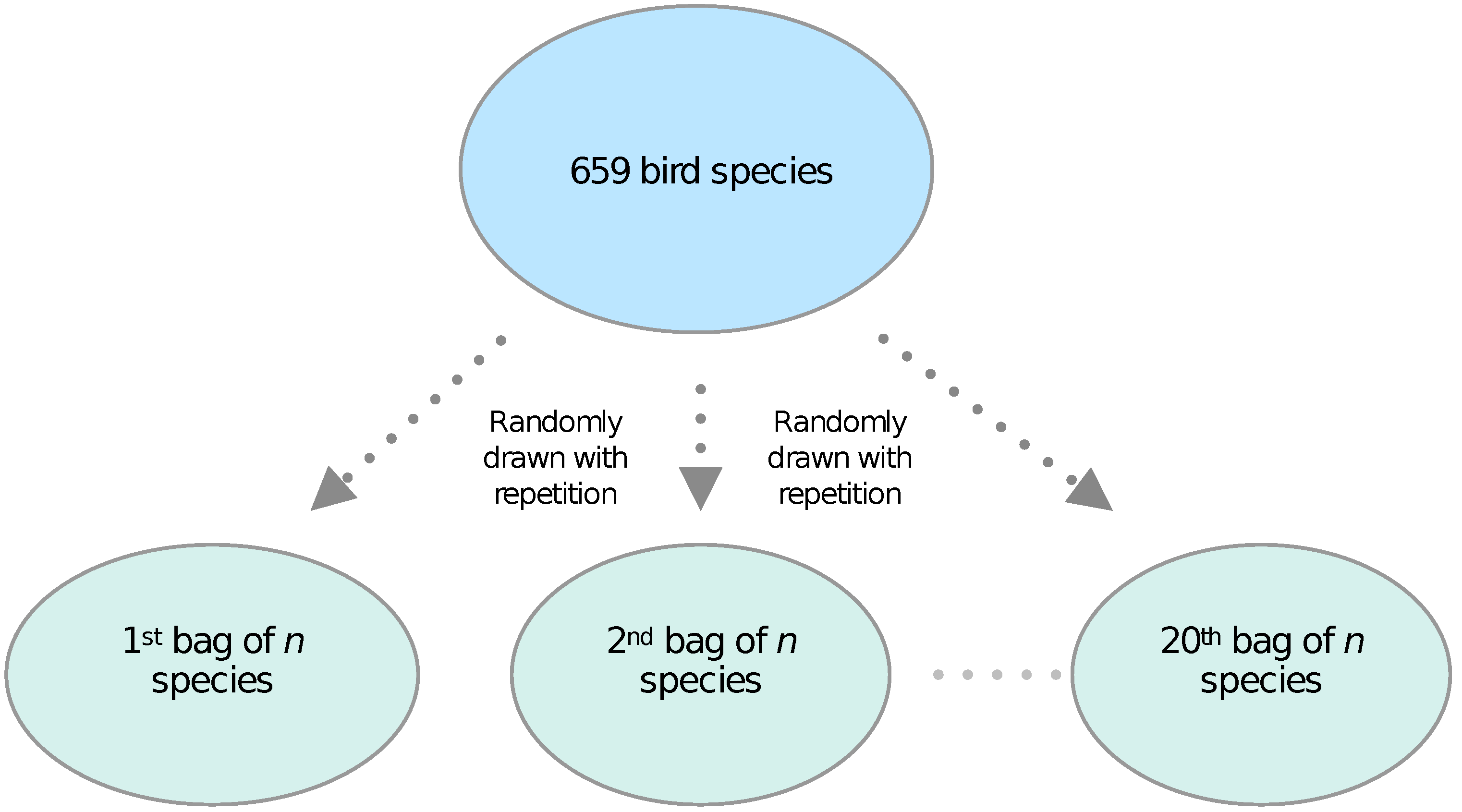
2.1. Bags-of-Birds Approach: Performing Randomized Classification Experiments

In this contribution, we used a dataset containing birds sounds of 659 species provided within the BirdClef 2019 challenge [15] and originally drawn from the Xeno-Canto [16] repository for bird sounds. The data were prepared, for our analysis, by splitting all sound recordings of varying lengths into 5-s chunks. The audio clips were then resampled to 22,050 Hz with the Librosa 0.6 audio processing package [17]. It has been reported that most birds vocalize in the frequency range of 0.5 to 10 kHz [18]. The resampling is followed by peak normalisation. To remove sound samples that do not contain any bird sounds, a simple signal-to-noise ratio based estimate is employed. This estimate ensures with high probability that 5-s clips that do not contain bird sounds are discarded [19].

Since one of the aims of this work is to estimate the robustness of the classification approach, for each classification run of n species, the subsets of species were not carefully chosen. Rather, a random number generator is employed to construct 20 bags of species. Analogously to bag-of-words approaches, one can refer to this procedure as a bag-of-birds approach. Each bags-of-birds is basically a set of randomly drawn species without repetition from a complete list of 659 bird species. The idea is to repeat the computation 20 times to have a reliable estimate of classification performance given a certain number of species. Figure 1 illustrates the idea of this numerical experiment.

A balanced dataset was curated for the classification task in which 200 sound samples were randomly drawn for each bird species. Finally, the dataset was divided into training and testing sets such that the training sets contain 75% and test sets contain 25% of data. Given that, for each bird species, we are using 200 sound samples, the test set for each analyzed species will consequently contain $m=50$ sound samples. This is described in detail in Section 2.4.

2.2. Feature Extraction

The next step entails extracting audio features from time series of audio signals. Extracting features allows us to obtain lower-dimensional compact statistical representations while preserving the distinguishing characteristics of the signal in a non-redundant manner. In addition to reducing the computational costs, feature extraction can maximize the classification performance of the system [20]. Studies have shown that aggregated features allow us to achieve a better classification performance compared to a single feature [21]. In this contribution, we employ the spectral centroid, the spectral rolloff, the zero-crossing-rate, Spectral Bandwidth, the root-mean-square energy (RMSE), and the Mel-frequency-cepstral-coefficients (MFCCs) as features.

Since signal statistics change rapidly, bird sounds, like audio signals in general, are non-stationary signals. For this reason, feature extraction is performed in a short-term processing manner where the signal is chunked into short analysis frames. The analysis frames are assumed to be in a quasi-stationary state [22]. In order to preserve as much information and arrive at a sufficient trade-off between the frequency and temporal resolution, we selected an analysis frame size of 512 samples (23 ms) while allowing an overlap of 25%.

Therefore, the spectral features described below are computed frame wise. In the case an additional splitting into even shorter windows within each analysis frame is required (e.g., for the MFCC), the temporal average of the feature is computed to generate a single value that is associated with the respective analysis frame. For each MFCC, the variance of the coefficients within the analysis frame is also computed and used as an additional feature.

In more detail, all features are computed using the Librosa 0.6 audio processing package [17] and can be described as follows [22]:

• Spectral Centroid: The spectral centroid measures the frequency where the energy of a spectrum is centered. In other words, it localizes the center of mass of the spectrum and is calculated as a weighted mean of the frequencies that the signal is composed of:

  $$s_c=\frac{{\sum }_{k}S\left(k\right)f\left(k\right)}{{\sum }_{k}S\left(k\right)},$$

  (1)

  where $S\left(k\right)$ is the spectral magnitude at frequency bin k, and $f\left(k\right)$ represents the center frequency of the bin [23].
• Spectral Rolloff: The spectral rolloff gives the frequency $f\left(k\right)$, below which, a pre-defined percentage (usually set to 85%) of the total spectral energy is concentrated [24].
• Zero-Crossing Rate: The zero-crossing rate r measures the smoothness of a signal. It is the rate at which a signal changes its sign from negative to positive or vice versa [25].
• The root-mean-square energy (RMSE): The root-mean-square energy of a signal gives the signal’s total energy and is defined as:

  $$e_{rms}=\sqrt{2\sum _k{\left|S\left(k\right)\right|}^2},$$

  (2)

  where $S\left(k\right)$ is the spectral magnitude at frequency bin k [17].
• Spectral Bandwith: measures if the power spectrum is concentrated around the spectral centroid or spread across the spectrum. It is computed as:

  $$s_b=\sqrt{\frac{{\sum }_k{\left(k-s_c\right)}^2·{\left|S\left(k\right)\right|}^2}{{\sum }_k{\left|S\left(k\right)\right|}^2}},$$

  (3)

  where $s_c$ is the spectral centroid, $S\left(k\right)$ is the spectral magnitude at frequency bin k [26].
• Mel-Frequency Cepstral Coefficients (MFCCs): Mel-Frequency Cepstral Coefficients are inspired by human auditory perception. After computing the Fourier transform of a signal, the magnitude spectrum is projected to the Mel scale, which emphasizes relevant frequencies in a non-linear way—a small bandwidth at low frequencies and large bandwidth at high frequencies. The Mel scale approximates human auditory response better than linearly spaced frequency bands. The output is log transformed, and MFCCs are obtained by taking a discrete cosine transform of the logarithmic outputs [27]. In this contribution, the analysis frames are split into windows of lengths 512 and compute the first 20 MFCC values as features in our system.

In total, the dimensions of the feature space are 45, containing first 20 time averaged MFCCs, variances of first 20 MFCCs, and the time-averaged zero-crossing-rate, the spectral rolloff, the spectral centroid, the root-mean-square energy, and the spectral bandwidth.

2.3. Classification Model

The features are then fed into a feed forward neural network, which is constructed using the sequential model within the Tensor Flow framework [28]. Feed forward neural networks are archetypal models for machine learning [29,30]. In contrast to the deep learning approaches used to classify bird sounds, the network consists of only four layers as illustrated in Figure 2. These constitute a sequence of layers where each layer is an affine transformation followed by a non-linear transfer function $\sigma$:

$$f_i(\overrightarrow{x}\mid \theta ):={\sigma }_i\left({\overrightarrow{w}}_i^{\top }\overrightarrow{x}+{\overrightarrow{b}}_i\right)$$

, $\theta =({\overrightarrow{w}}_i,{\overrightarrow{b}}_i,{\sigma }_i)$ constitutes the parameter space where ${\overrightarrow{w}}_i$ are weights, ${\overrightarrow{b}}_i$ are biases, and ${\sigma }_i$ are transfer functions for different layers i. The goal of the neural network is to learn the value of parameter $\theta$ that generates the best function approximation [22,31]. The input to the neural network is the feature vector $\overrightarrow{x}\in {\mathbb{R}}^{45}$, which maps through three intermediate layers with $d_1=256$, $d_2=128$, and $d_3=64$ hidden units, respectively, and is amplified using rectified linear units (ReLU) [31]. Finally, the output layer maps to n independent classes with a softmax transfer function [31,32] where n is the number of bird species.

During training, the model optimizes the cross-entropy loss using the Adam stochastic optimization algorithm [33]. We used a constant learning rate of 0.001. To identify the parameter setting that increases the likelihood of predictions, the model was trained for 100 epochs. We observed, from our experiments, that the loss converged to a minimum toward the end of 100 epochs.

2.4. Measuring Classification Success

This section introduces the indices used to measure the classification performance of bird vocalizations [34,35]. In each numerical experiment, we considered n species and a dataset of a total of $4m$ sound samples. In more detail, $3m$ samples were used for training, whereas the remaining m samples were employed to evaluate the quality of classifications. Within the dataset for n randomly selected species, for each species $j=1,2,...,n$, a dataset of $4m$ samples was processed. Here, $3m$ samples were used for training, whereas the remaining m samples were employed to evaluate the quality of the classifications. These evaluations were then done by computing a confusion matrix for each species, containing:

$c_{tp}\left(j\right)$	the number of classifications that are true positives for species j,
$c_{tn}\left(j\right)$	the number of classifications that are true negatives for species j,
$c_{fp}\left(j\right)$	the number of classifications that are false positives for species j, and
$c_{fn}\left(j\right)$	the number of classifications that are false negatives for species j.

The resulting elements of the confusion matrix enter into computation of more advanced metrics for measuring classification success, such as the precision, recall, accuracy, mean-average-precision, and receiver-operator characteristics. To understand how the entries of each species’ confusion matrix influence the outcomes of these summarizing measures, more detailed descriptions of their computations are introduced in the following:

• Precision: This metric gives the measure of reliability of our predictions. The formula to compute the precision for a bird species j is

  $$p\left(j\right):=\frac{c_{tp}\left(j\right)}{c_{tp}\left(j\right)+c_{fp}\left(j\right)}.$$

  (4)
  Therefore, the precision for a species j indicates how many true positives the model predicted out of all positives. Therefore, the higher the precision, the more confident a model is about its predictions. In order to compute the precision for the entire test dataset, we average over all species

  $$P=\frac{1}{n}\sum _{j=1}^{n}p\left(j\right).$$

  (5)
• Recall: This metric gives the measure of predictive power of a model. The formula to compute recall for each bird species j is

  $$r\left(j\right):=\frac{c_{tp}\left(j\right)}{c_{tp}\left(j\right)+c_{fn}\left(j\right)}.$$

  (6)
  Thus, to recall, for a class species j, would indicate, of all actual positives in the test dataset, how many did the model predict as positive. Therefore, the higher the recall, the more positive samples the model correctly classified as positive. In order to compute the recall for the entire test dataset, we averaged over all species

  $$R=\frac{1}{n}\sum _{j=1}^{n}r\left(j\right).$$

  (7)
• Accuracy: While precision and recall are computed for each class separately in a multi-class classification problem, the accuracy A is computed for the entire test dataset using

  $$A:=\frac{{\sum }_{j=1}^n{c}_{tp}\left(j\right)}{m·n}.$$

  (8)

  and thus, out of all test samples, how many were correctly classified.
• Area Under ROC Curve (AUC): An ROC curve shows the performance of a classification model at different classification thresholds. The curve is computed by plotting the true positive rate ($r_{tp}$) against the false positive rate ($r_{fp}$) at these thresholds. The true positive rate for a bird species j is defined as:

  $$r_{tp}(j,\rho ):=\frac{c_{tp}(j,\rho )}{c_{tp}(j,\rho )+c_{fn}(j,\rho )},$$

  (9)

  and the false positive rate for a bird species j is defined as

  $$r_{fp}(j,\rho ):=\frac{c_{fp}(j,\rho )}{c_{fp}(j,\rho )+c_{tn}(j,\rho )},$$

  (10)

  with $\rho$ denoting a probability threshold that is varied from 0 to 1 in order to obtain the ROC curve. The area under the ROC curve (AUC) gives an aggregate measure of the classification performance.
  The ROC was originally developed for a binary classifier and was later generalized for a multi-class classification system [36]. The test set labels are binarized by employing either the one-vs-one or the one-vs-rest configuration. We employed the one-vs-one configuration for our task. In more detail, different sound samples are ranked by their probabilities, and then false positive and true positive rates are computed by choosing different probability cut-offs $\rho$ to generate the ROC curve. The AUC is computed as the area under the ROC curve. In the end, an average across species is computed to get one AUC value for the entire data set, i.e.,

  $$AUC=\frac{1}{n}\sum _{\rho }\sum _{j=1}^n{r}_{tp}(j,\rho ).$$

  (11)
• Mean Average Precision (mAP): The evaluation metric gives us a way of characterizing the performance of a classifier by monitoring how precision changes with varying the classification probability threshold that the model uses to make a decision if a bird sound sample belongs to a class j. A good classifier will maintain a high precision as recall increases, while a poor classifier will take a hit on precision as recall increases with changes in threshold.
  In more detail, to compute Average Precision for a species j, a list of probabilities is generated in which the discrimination probabilities our model has assigned to all test samples for class j are stored. The list is then sorted by decreasing probabilities, and each element is assigned a rank k. By varying the rank k (by gradually lowering the probability threshold), a list of true positives and false positives is generated. Note that, as the classification threshold is lowered, the model labels increasingly more samples as positive. This will lead to an increase in false positives. The list is consequently employed to produce a list of precision values at different ranks $p\left(k\right)$. Considering all the K cases in the list where the sound sample belongs to class j, the average precision is computed as:

  $$P_A\left(j\right):=\frac{{\sum }_{k=1}^{K}p\left(k\right)\mathbf{1}\left(k\right)}{c_{tp}\left(j\right)},$$

  (12)

  where $\mathbf{1}\left(k\right)$ is an indicator function that equals unity if the sample at threshold k is a true positive. The mean average precision $P_{mA}$ is then computed by averaging over all classes (species) [15].

  $$P_{mA}:=\frac{{\sum }_{j=1}^n{P}_A\left(j\right)}{n}.$$

  (13)

3. Results and Discussion

We evaluated the performance of our classification algorithm by testing it for 20 trials on n randomly selected species, (out of 659 species in the selected dataset) with n varying between $n=10$ and $n=300$. The results for the precision, AUC, mAP, recall, and accuracy are summarized in Figure 3.

Box plots were estimated from 20 different randomized data sets for each n. Box plots, also known as box-and-whisker plots, provide robust statistical summaries for the data, if the sample size is relatively small, i.e., here 20. The box plot divides the data into quartiles or fourths—two box panels and two whiskers. The middle 50% of data is spanned by the box with the 25th percentile or 25% of the data falling below the lower edge of the box (first quartile) and 75% of data falling below the upper edge of box (third quartile). The edges of the box are often referred to as hinges, and the length of the box is called the interquartile range (IQR). The median is indicated by the middle line of box. The whiskers mark the extremes for the remaining 50% of the data [37]. Surprisingly, we found no increase in the size of the interquartile range for the performance measures with increasing n.

There are several aspects of these results that deserve to be addressed in more detail.

3.1. Variations due to Randomized Sub-Sets

As observed in Figure 3, we can see that, for each choice of a subset of n species, we obtain a range of performance values, depending on the particular random selection of species. Our results show that the interquartile ranges vary as much as 12% in some cases. For instance, in case of $n=30$ in Figure 3c, we see that the mean average precision (mAP) varies between 0.72 for one subset of 30 species to 0.84 for another subset of randomly drawn 30 species. Similarly for n = 70, the mAP varies between 0.6 and 0.71. We can see a similar trend in the figures for other metrics considered in this work.

As mentioned earlier, the experiment was repeated 20 times for different randomized selections of n species. The variation in results within different n species’ trials showed that the classification results can vary significantly depending on the choice of species chosen for the analysis. Consequently, it can be inferred that generic claims about the performance of a certain algorithm for a certain number of non-randomly selected species must be interpreted with caution. The results might not generalize for another set of n species, even when the species are drawn from the same dataset.

One possible reason, among others, that could explain the variability in performance between different subsets or ensembles of randomly drawn sound samples from n species (bag-of-birds) is the possible degrees of similarity of sounds, or the lack of it, between species of different subsets. Ambiguity can be a consequence of the similarity of the sounds of species within an ensemble. Therefore, one possible explanation for these results is that sounds of species in the bags leading to lower performance measures have a higher degree of similarity compared to bags that generate higher classification performance.

3.2. The Dependence on the Number of Species

All performance measures decrease with an increased number of species as is visible in Figure 3 and Figure 4.

An intuitive explanation for this could be that species are more difficult to distinguish when more species are added to the classification task. However, looking at the definitions of the performance measures (Equations (4)–(13)) we investigated whether it is possible to understand the numerical results by analytic reasoning. Consider, e.g., the precision $P\left(n\right)$, which is defined in Equation (5). If each precision per species $p\left(j\right)$ contributing to the average is constant and not depending on n (i.e., $p\left(j\right)\sim c$), one should expect $P\left(n\right)\sim c$. This is clearly not what is observed in Figure 4. Therefore, one must assume that $p\left(j\right)$ is dependent on n, although this is not explicitly visible in Equation (4). To investigate this implicit dependence on n, we visualized the average numbers of true positives

$$a_{tp}=\frac{1}{n}\sum _{j=1}^n{c}_{tp}\left(j\right),$$

(14)

for each n and, in a similar way, the averaged numbers of false positives, true negatives, and false negatives in Figure 5a–c. These elements of a confusion matrix enter (in an non-averaged form) into the computed performance measures, and thus their dependence on n influences the performance measures. The averaging in Figure 5 was done, since the amount of sound samples in each trial clearly depends linearly on n. Therefore, this trivial dependence was removed, and we can monitor a non-trivial implicit dependence on n.

As one can see, the dependence of the averaged numbers of true positive, false positives, and false negatives can be described relatively well by a quadratic function, whereas the averaged number of true negatives increases linearly with increasing n.

The fact that true negatives, as can be seen in Figure 5d, behave differently than the other elements of the confusion matrix can be understood by considering the way true negatives are computed in a multi-class classification problem, using a one-vs-all configuration. Each time a sound sample was correctly not classified as the particular species j under consideration, the count of true negatives was increased by one. Therefore, e.g., in a subset of $m·n=500$ sound samples recorded from $n=10$ different species and each species being represented by $m=50$ sound samples, a perfect algorithm would classify 50 samples correctly as belonging to species j. Consequently, the count of true positives would be $c_{tp}\left(j\right)=50$, and the count of true negatives $c_{tn}\left(j\right)=450$ for a perfect classifier. In other words, we can expect $c_{tn}\left(j\right)=nm-m$ with m being the sample size, as specified before, in case of a perfect classifier

$$a_{tn}=\frac{1}{n}\sum _{i=1}^{n}nm-m=\frac{n(nm-m)}{n}=m(n-1).$$

(15)

The results of the prediction experiments in this contribution with an obviously not perfect classifier, reveal that $a_{tn}$ can be fitted by a linear function $a_{tn}\left(n\right)=b_{1}n+b_0$, where $b_1=(49.88\pm 0.82)\times {10}^{-2}$, and $b_0=-(59.27\pm 0.61)$. Note that the two coefficients are relatively close to the true sample size $m=50$.

The dependence of the other elements of the confusion matrix on n are more subtle with respect to the range in which these numbers vary, and the dependence can be described by quadratic functions

$$\begin{array}{ccc}\hfill a_{tp}\left(n\right)& =& d_2{n}^2-d_{1}n+c_0,\hfill \end{array}$$

(16)

$$\begin{array}{ccc}\hfill a_{fp}\left(n\right)& =& -d_2{n}^2+d_{1}n+d_0\mathrm{and},\hfill \end{array}$$

(17)

$$\begin{array}{ccc}\hfill a_{fn}\left(n\right)& =& -d_2{n}^2+d_{1}n+d_0,\hfill \end{array}$$

(18)

with $d_2=(8.02\pm 1.00)\times {10}^{-4}$, $d_1=(22.87\pm 1.34)\times {10}^{-2}$, $d_0=6.84\pm 0.37$ and $c_0=43.16\pm 0.38$. Note that the first two coefficients $d_1$ and $d_2$ of $a_{tp}$, $a_{fp}$ and $a_{fn}$ have either the same values (up to the first eight digits, which are not shown here), or just differ in sign but not in value. These coefficients are shown in detail here since we will, in the following, demonstrate a connection between Equations (16)–(18) and the functions describing the dependence of the overall performance measures.

Being able to describe $a_{tp}\left(n\right)$, $a_{fp}\left(n\right)$ and $a_{fn}\left(n\right)$, one can now attempt to understand the dependencies of the performance measures. Assuming that each species is classified equally well by a perfect classifier, one would expect $a_{tp}\left(n\right)=c_{tp}(j,n)$ for all j and similar for $a_{fp}=c_{fp}(j,n)$ and $a_{fn}=c_{fn}$. Inserting Equations (16) and (17) in Equation (4) holds

$$p(j,n)\approx \frac{a_{tp}\left(n\right)}{a_{tp}\left(n\right)+a_{fp}\left(n\right)}\approx \frac{d_2{n}^2-d_{1}n+c_0}{c_0+d_0},$$

(19)

since the non-constant terms in the denominator cancel each other. Inserting this in the equation for the overall precision (Equation (5)) holds

$$P\left(n\right)\approx \frac{d_2{n}^2-d_{1}n+c_0}{c_0+d_0}\sim a_{tp}\left(n\right),$$

(20)

since all terms $p\left(j\right)$ are identical for the perfect classifier. Consequently, one should be able to predict the scaling of $P\left(n\right)$, knowing the coefficients $d_2,d_1,d_0$, and $c_0$.

Fitting the coefficients for the quadratic function describing $P\left(n\right)$ as in Figure 4, one obtains

$$P\left(n\right)\approx g_2{n}^2+g_{1}n+g_0,$$

(21)

with $g_2=(0.16\pm 0.02)\times {10}^{-4}$, $g_1=-(0.44\pm 0.03)\times {10}^{-2}$, $g_0=0.86\pm 0.76\times {10}^{-2}$. Note that these coefficients are very close to the coefficients of $a_{tp}$ multiplied with a factor $\frac{1}{d_0+c_0}=\frac{1}{50}$ as indicated by Equation (20). Hence, we can confirm numerically that the dependence of the precision on the number of classes follows the dependence of $a_{tp}$ up to a scaling factor of $\frac{1}{d_0+c_0}=\frac{1}{50}$.

Following the same assumptions and reasoning, one obtains

$$R\left(n\right)\approx r\left(j\right)\approx \frac{d_2{n}^2-d_{1}n+c_0}{c_0+d_0}\sim a_{tp}\left(n\right),$$

(22)

for the recall. Here, the relation between the fitting coefficients of $a_{tp}$ and R is confirmed by the quadratic function fitted to R in Figure 4. Note that, for the prediction experiments in this study, the same quadratic function is able to describe the n-dependence of precision and recall.

Extending the above reasoning (i.e., $c_{tp}(j,n)\approx atp\left(n\right)$) to explain the n-dependence of the accuracy as given by Equation (8) yields

$$A\left(n\right)\approx \frac{1}{m}\left(d_2{n}^2-d_{1}n+c_0\right)\sim a_{tp}\left(n\right).$$

(23)

This relation was numerically confirmed by comparing the coefficients for the polynomials describing A and $a_{tp}$. The values of coefficients $d_2$, $d_1$, and $c_0$ are given after Equation (18).

Discussing the n-dependence of the multi-class AUC and the mAP analytically is not as straightforward as the previous considerations; therefore, only numerical results are presented in this contribution. As one can see in Figure 4, the n-dependence of AUC and mAP can be also described by quadratic functions. Additionally, we observe that the coefficients for the linear and the quadratic term of the function describing the mAP resemble the coefficients describing $P\left(n\right)$ in value (The values describing coefficients of $P\left(n\right)$ are given after Equation (21)). Consequently, one can argue that the above discussion for $P\left(n\right)$ could possibly also explain the n-dependence of mAP. Nevertheless, the constant term ($c_0=43.16\pm 0.38$) added to the function describing $P_{mA}\left(n\right)$ is higher than the constant offset of the precision.

Summarizing, we can relate the n-dependence of several measures for the classification success to the n-dependences of the confusion matrix, assuming the behaviour of a perfect classifier, and we fit functions describing these dependencies. Note that this does not imply that we claim our classifier to be a perfect classifier, neither do we claim that scaling with n, which we obtain here, is universal in the sense that it will be observed for any other classifier. The latter aspect is a question that needs to be tested in future contributions, but it is out of the scope of this work.

3.3. Metric of Confidence

The decisions made by the classifier are based on probabilities that are estimated (through the ANN) for each species. The predicted label is then assigned to the species with the highest probability. Here, we analyze the effect of introducing a confidence threshold requiring the assigned probability to be above the threshold in order to accept the classification. In Figure 6, one can see that the precision (cTPS/cPs), i.e., the ratio of true positives to all classified positives changes as the confidence threshold is varied between 0.5 and 1.0.

We see that the precision increases as the confidence threshold is increased. For instance, for $n=30$ species, the precision for a confidence threshold in range of 0.9–1.0 is more than 0.8. Similar results can be seen for other n. This basically shows that when the model is assigning high confidence to its predictions, the predictions are mostly correct, which should be expected from a good classifier.

3.4. Comparing Different Measures for Classification Success

In this contribution, we used several common measures for evaluating the classification performance and comparing their results. The primary reason for this is that different indices encapsulate different aspects of the classification performance. Secondly, as mentioned earlier, there seems to be no consensus in the literature available on the choice of evaluation metric for the audio-based bird species classification task. This compelled us to study a set of indices and not rely on a specific metric.

As one can see in Figure 3, the precision and recall for $n<100$ do not show much disparity and instead look quite similar.

Although, by definition, these two indices encapsulate different aspects of model performance. This can be clearly seen in Figure 7. Here, we see that for different species in one classification run of $n=10$, the precision and recall values differ. There are species where the precision is higher than the recall (e.g., species 10) while others where the recall is higher than the precision (e.g., species 3). It seems that, for $n<100$, the precision and recall values more or less equalize when an average is taken over a species.

From Figure 3 and Figure 4, one can additionally see that the accuracy is exactly the same as the recall, since the equations of recall and accuracy become the same when averages are taken over all classes.

Additionally, the mean average precision (mAP) was used to evaluate classification success. Increasingly a number of works in recent years have used this metric to state the classification performance of their models. Note that average precision is one way of measuring the area under the precision–recall curve. Compared to precision and recall that are computed for one probability threshold, the average precision is computed cumulatively by varying the threshold. We see in Figure 3 that, although it follows a similar downward quadratic trend to the recall and precision, the mAP values are slightly higher than the precision and recall values for different n. For instance, the range for $n=10$ species for the 20 runs is between 0.86 and 0.94, whereas the precision and recall ranges are between 0.79 and 0.87. This observation also reflected in the offset of the functions describing the n-dependence as mentioned above.

Another commonly used metric for classification success is the area under the Receiver Operating Characteristics curve (AUC). Our model achieved a high score on the AUC metric as can be seen in Figure 3 and Figure 4. Although the AUC score decreased with the increase in number of species n, the score was nevertheless unexpectedly high. For instance, the AUC score for n = 300 for one run was 0.94, which is unexpected for such a large number of species. (Note that, as per the definition of the AUC, a random classifier making randomized decisions should give a score of 0.5).

In our understanding, the multi-class nature of our problem explains this result. As mentioned earlier, the AUC metric was essentially designed for a binary classifier and was later generalized for multi-class classification problems [36].

Therefore, in the case of multi-class problems one needs to binarize the class labels to compute the AUC score, such that the problem is transformed into a binary classification problem with $\frac{n(n-1)}{2}$ binary classifiers (where n is number of classes). Using a one-vs-one configuration [36,38], as recommended by tutorials of many software packages, an AUC score is then computed for each of these binary classifiers, and finally an average is computed to obtain a final AUC score for the entire set of n classes.

For an actual binary classifier that classifies poorly, the miss-classifications will reflect in significant enough values of false positives and false negatives to give us a low true positive rate and high false positive rate as per Equations (9) and (10). This will result in a low AUC score. In the multi-class scenario with one-vs-one configuration, we observe that a classifier distributing miss-classifications sparsely across several classes leads to a small number of false positives and small number of false negatives for these artificially assumed binary classifiers. One should note that this will happen even if the classifier fairs poorly i.e., miss-classifies with a high rate.

An example for this can be seen in Figure 8, which shows a confusion matrix for a classification run with 20 species. It can be seen that the miss-classifications are spread throughout the rows and columns of the confusion matrix. Consequently, less numbers of false positives and false negatives will amount to a high true positive rate and low false positive rate for individual binary comparisons and, therefore, a high AUC score (refer to Equations (9) and (10)). This is exactly what is reflected on averaging the individual AUC scores to compute the total AUC score for n classes.

The classifier is distributing the false predictions sparsely across several classes and the one-vs-one generalization is unable to capture the actual performance of the model. This leads us to the conclusion that ROC is not a suitable performance measure for multi-class classification tasks. Especially in cases where the miss-classifications are distributed rather evenly among several classes, it is very likely to obtain overestimated AUC scores.

4. Conclusions

The novelty of this work lies in studying the dependence of classification success on the number of species for bird sound classification. Furthermore, the idea is to illustrate how these classification results are heavily contingent on the composition of bird species subsets. Therefore, we employed balanced subsets of bird sounds for n species, drawing the species randomly from a larger dataset containing 659 species, where n was varied between 10 and 300. For each n, we repeated the whole procedure (composition of the subset, training of the classifier, and testing) 20 times to produce a reliable estimate of the performance given a certain number of bird species.

The classification was performed using a shallow feed forward neural network trained on 45 pre-computed sound features. We used a shallow neural network to conduct our analysis primarily due to its model simplicity, lower computational costs, and relatively low amount of data that is required to train such networks vis a vis deep neural networks. We wanted to benchmark the classification performance and perform our analysis using a simple model that can be trained using hand crafted sound features.

We evaluated the classification performance using several common measures for classification success and also analyzed their dependence on n in detail. We observed that the classification performance was relatively high, even when many different species were present in the datasets under study and using relatively less data. This is an interesting result, since many recent approaches are based on deep neural networks trained on much larger datasets of images of spectrograms without any feature selection. This suggests that shallow neural networks trained on pre-computed sound features can also provide a robust approach to bird classification, which, at the same time, is inexpensive in terms of the computational costs and the amount of data used.

Concerning the robustness of the approach, we found that all measures of classification success showed a decline in value if the number of species present in the subset was increased. For some of these measures, this decline can be explained analytically knowing the n-dependence of the confusion matrix and assuming the behavior of an idealized perfect classifier.

Additionally, we observe that the classification success depends on the individual composition of the bird subsets and classification results can vary significantly depending on the choice of species chosen for the analysis. For this reason, it seems the generic claims about the performance of a certain algorithm for, say n species of non-randomly drawn species, must not be interpreted as a generalized measure of performance for any n species. The classification results might not generalize for another set of n species, even when the species are drawn from the same dataset.

References

1. Sutherland, W.J.; Newton, I.; Green, R. Bird Ecology and Conservation: A Handbook of Techniques; OUP Oxford: Oxford, UK, 2004; Volume 1. [Google Scholar]
2. Priyadarshani, N.; Marsland, S.; Castro, I. Automated birdsong recognition in complex acoustic environments: A review. J. Avian Biol. 2018, 49, jav-01447. [Google Scholar] [CrossRef] [Green Version]
3. Zhang, X.; Li, Y. Adaptive energy detection for bird sound detection in complex environments. Neurocomputing 2015, 155, 108–116. [Google Scholar] [CrossRef]
4. Jančovič, P.; Köküer, M. Automatic detection and recognition of tonal bird sounds in noisy environments. EURASIP J. Adv. Signal Process. 2011, 2011, 982936. [Google Scholar] [CrossRef] [Green Version]
5. Fox, E.J.; Roberts, J.D.; Bennamoun, M. Text-independent speaker identification in birds. In Proceedings of the Ninth International Conference on Spoken Language Processing, Pittsburgh, PA, USA, 17–21 September 2006. [Google Scholar]
6. Cai, J.; Ee, D.; Pham, B.; Roe, P.; Zhang, J. Sensor network for the monitoring of ecosystem: Bird species recognition. In Proceedings of the 2007 3rd International Conference on Intelligent Sensors, Sensor Networks and Information, Melbourne, VIC, Australia, 3–6 December 2007; pp. 293–298. [Google Scholar]
7. Chen, Z.; Maher, R.C. Semi-automatic classification of bird vocalizations using spectral peak tracks. J. Acoust. Soc. Am. 2006, 120, 2974–2984. [Google Scholar] [CrossRef] [PubMed]
8. Jančovič, P.; Köküer, M. Acoustic recognition of multiple bird species based on penalized maximum likelihood. IEEE Signal Process. Lett. 2015, 22, 1585–1589. [Google Scholar]
9. Wielgat, R.; Potempa, T.; Świétojański, P.; Król, D. On using prefiltration in HMM-based bird species recognition. In Proceedings of the 2012 International Conference on Signals and Electronic Systems (ICSES), Wroclaw, Poland, 18–21 September 2012; pp. 1–5. [Google Scholar]
10. Briggs, F.; Lakshminarayanan, B.; Neal, L.; Fern, X.Z.; Raich, R.; Hadley, S.J.; Hadley, A.S.; Betts, M.G. Acoustic classification of multiple simultaneous bird species: A multi-instance multi-label approach. J. Acoust. Soc. Am. 2012, 131, 4640–4650. [Google Scholar] [CrossRef] [PubMed] [Green Version]
11. Juang, C.F.; Chen, T.M. Birdsong recognition using prediction-based recurrent neural fuzzy networks. Neurocomputing 2007, 71, 121–130. [Google Scholar] [CrossRef]
12. Sprengel, E.; Jaggi, M.; Kilcher, Y.; Hofmann, T. Audio Based Bird Species Identification Using Deep Learning Techniques; Technical Report; CLEF: Evora, Portugal, 2016. [Google Scholar]
13. Bastas, S.; Majid, M.W.; Mirzaei, G.; Ross, J.; Jamali, M.M.; Gorsevski, P.V.; Frizado, J.; Bingman, V.P. A novel feature extraction algorithm for classification of bird flight calls. In Proceedings of the 2012 IEEE International Symposium on Circuits and Systems (ISCAS), Seoul, Korea, 20–23 May 2012; pp. 1676–1679. [Google Scholar]
14. Selin, A.; Turunen, J.; Tanttu, J.T. Wavelets in recognition of bird sounds. EURASIP J. Adv. Signal Process. 2006, 2007, 1–9. [Google Scholar] [CrossRef] [Green Version]
15. Kahl, S.; Stöter, F.R.; Goëau, H.; Glotin, H.; Planque, R.; Vellinga, W.P.; Joly, A. Overview of BirdCLEF 2019: Large-scale bird recognition in soundscapes. In Proceedings of the Working Notes of CLEF 2019-Conference and Labs of the Evaluation Forum, CEUR, Lugano, Switzerland, 9–12 September 2019; pp. 1–9. [Google Scholar]
16. Xeno Canto. Available online: https://www.xeno-canto.org/ (accessed on 27 May 2020).
17. McFee, B.; McVicar, M.; Balke, S.; Thomé, C.; Raffel, C.; Lee, D.; Nieto, O.; Battenberg, E.; Ellis, D.; Yamamoto, R.; et al. Librosa/Librosa: 0.6.3. 2019. Available online: https://doi.org/10.5281/zenodo (accessed on 21 June 2021).
18. Marler, P.R.; Slabbekoorn, H. Nature’s Music: The Science of Birdsong; Elsevier: Milano, Italy, 2004. [Google Scholar]
19. Kahl, S.; Wilhelm-Stein, T.; Klinck, H.; Kowerko, D.; Eibl, M. Recognizing birds from sound-the 2018 BirdCLEF baseline system. arXiv 2018, arXiv:1804.07177. [Google Scholar]
20. Khalid, S.; Khalil, T.; Nasreen, S. A survey of feature selection and feature extraction techniques in machine learning. In Proceedings of the 2014 Science and Information Conference, London, UK, 27–29 August 2014; pp. 372–378. [Google Scholar]
21. Xie, J.; Zhu, M. Handcrafted features and late fusion with deep learning for bird sound classification. Ecol. Informatics 2019, 52, 74–81. [Google Scholar] [CrossRef]
22. Virtanen, T.; Plumbley, M.D.; Ellis, D. Computational Analysis of Sound Scenes and Events; Springer: Cham, Switzerland, 2018. [Google Scholar]
23. Klapuri, A.; Davy, M. Signal Processing Methods for Music Transcription; Springer: New York, NY, USA, 2007. [Google Scholar]
24. Smith, J.O. Spectral Audio Signal Processing, 2011 ed.; Online Book; W3K Publishing: Palo Alto, CA, USA, 2011; Available online: http://ccrma.stanford.edu/~jos/sasp/ (accessed on 23 July 2021).
25. Giannakopoulos, T.; Pikrakis, A. Introduction to Audio Analysis: A MATLAB® Approach; Academic Press: Cambridge, MA, USA, 2014. [Google Scholar]
26. Abreha, G.T. An Environmental Audio-Based Context Recognition System Using Smartphones. Master’s Thesis, University of Twente, Enschede, The Netherlands, 2014. [Google Scholar]
27. Logan, B. Mel Frequency Cepstral Coefficients for Music Modeling; ISMIR: Plymouth, MA, USA, 2000; Volume 270, pp. 1–11. [Google Scholar]
28. Abadi, M.; Barham, P.; Chen, J.; Chen, Z.; Davis, A.; Dean, J.; Devin, M.; Ghemawat, S.; Irving, G.; Isard, M.; et al. Tensorflow: A system for large-scale machine learning. In Proceedings of the 12th {USENIX} Symposium on Operating Systems Design and Implementation ({OSDI} 16), Savannah, GA, USA, 2–4 November 2016; pp. 265–283. [Google Scholar]
29. Bebis, G.; Georgiopoulos, M. Feed-forward neural networks. IEEE Potentials 1994, 13, 27–31. [Google Scholar] [CrossRef]
30. Fine, T.L. Feedforward Neural Network Methodology; Springer Science & Business Media: New York, NY, USA, 2006. [Google Scholar]
31. Goodfellow, I.; Bengio, Y.; Courville, A.; Bengio, Y. Deep Learning; MIT Press: Cambridge, MA, USA, 2016; Volume 1. [Google Scholar]
32. Bishop, C.M. Pattern Recognition and Machine Learning; Springer: Berlin/Heidelberg, Germany, 2006. [Google Scholar]
33. Kingma, D.P.; Ba, J. Adam: A method for stochastic optimization. arXiv 2014, arXiv:1412.6980. [Google Scholar]
34. Performance metrics for classification problems in machine learning. Available online: https://medium.com/thalusai/performance-metrics-for-classification-problems-in-machine-learningpart-i-b085d432082b (accessed on 15 July 2021).
35. Grandini, M.; Bagli, E.; Visani, G. Metrics for Multi-Class Classification: An Overview. arXiv 2020, arXiv:stat.ML/2008.05756. [Google Scholar]
36. Hand, D.J.; Till, R.J. A simple generalisation of the area under the ROC curve for multiple class classification problems. Mach. Learn. 2001, 45, 171–186. [Google Scholar] [CrossRef]
37. Nuzzo, R.L. The box plots alternative for visualizing quantitative data. PM&R 2016, 8, 268–272. [Google Scholar]
38. Pedregosa, F.; Varoquaux, G.; Gramfort, A.; Michel, V.; Thirion, B.; Grisel, O.; Blondel, M.; Prettenhofer, P.; Weiss, R.; Dubourg, V.; et al. Scikit-learn: Machine Learning in Python. J. Mach. Learn. Res. 2011, 12, 2825–2830. [Google Scholar]
Figure 1. Schematic for the bags-of-birds approach.
Applsci 11 09226 g001
Figure 2. The architecture of the feed forward neural network used for bird classification. The input x R 45 maps through three intermediate layers with d 1 = 256 , d 2 = 128 , and d 3 = 64 and ReLU transfer functions. The output layer maps to n independent classes with a softmax transfer function where n is the number of bird species.
Applsci 11 09226 g002
Figure 3. The performance measures (a) Precision (b) AUC (c) mAP (d) Recall and (e) Accuracy decrease as the number of species in each subset is varied between n = 10 and n = 300 . Shown are the ranges from best result to worst result (whiskers) obtained for 20 different randomly drawn subsets for each value of n. The red marking in each box represents the median, and the boxes indicate the middle 50% of the results.
Applsci 11 09226 g003
Figure 4. The n-dependence of (a) Precision, (b) AUC, (c) mAP, (d) Recall and (e) Accuracy can be described by fitting quadratic functions (line). The error bars (whiskers) represent the ranges from the best result to worst result obtained for 20 different randomly drawn subsets for each value of n. The red marking in each box indicates the median, and the boxes show the range of the middle 50% of the results.
Applsci 11 09226 g004
Figure 5. The elements of a confusion matrix (a) averaged numbers of true positives, (b) averaged numbers of false positives, (c) averaged numbers of false negatives, (d) averaged numbers of true negatives) display a linear (true negatives) and quadratic (all other elements) dependence on n. The error bars (whiskers) represent the ranges from the best result to worst result obtained for 20 different randomly drawn subsets for each value of n. The green marking in each box indicates the median, and the boxes show the range of the middle 50% of the results.
Applsci 11 09226 g005
Figure 6. The precision (cTPs/cPs) increases as the confidence threshold (probability a sample needs to be assigned by the model in order for it to be classified as a positive prediction) is varied between 0.5 and 1.0. Shown are precision values for n = 30 , 60 , 90 , and 300. As we can see for different n, as the confidence threshold tends toward 1.0, the precision also increases significantly.
Applsci 11 09226 g006
Figure 7. The precision, recall, and average precision for individual species classified in a subset composed of 10 randomly selected species are compared. The largest and the smallest value of each performance measure indicate a relatively large variation and strong dependence on the particular species under study.
Applsci 11 09226 g007
Figure 8. The confusion matrix for a classification run with n = 20 species displays that the miss-classifications are spread among several classes. This can result in an overestimation of the averaged AUC for multi-class classifications.
Applsci 11 09226 g008
Publisher’s Note: MDPI stays neutral with regard to jurisdictional claims in published maps and institutional affiliations.