A Robot-Assisted Large-Scale Inspection of Wind Turbine Blades in Manufacturing Using an Autonomous Mobile Manipulator

Abstract

Wind energy represents the dominant share of renewable energies. The rotor blades of a wind turbine are typically made from composite material, which withstands high forces during rotation. The huge dimensions of the rotor blades complicate the inspection processes in manufacturing. The automation of inspection processes has a great potential to increase the overall productivity and to create a consistent reliable database for each individual rotor blade. The focus of this paper is set on the process of rotor blade inspection automation by utilizing an autonomous mobile manipulator. The main innovations include a novel path planning strategy for zone-based navigation, which enables an intuitive right-hand or left-hand driving behavior in a shared human–robot workspace. In addition, we introduce a new method for surface orthogonal motion planning in connection with large-scale structures. An overall execution strategy controls the navigation and manipulation processes of the long-running inspection task. The implemented concepts are evaluated in simulation and applied in a real-use case including the tip of a rotor blade form.

1. Introduction

Wind energy has gradually taken the dominant share of renewable energies. The worldwide capacity increased from 7600 MW in 1998 to 93 GW in 2020 [1]. The main components of a wind turbine are: a rotor equipped with wing-shaped blades, a nacelle that houses a drive train, and a tower [2]. The rotor blades transform the wind energy into rotary energy and must be lightweight, robust, and long-lasting. Therefore, they are made from composite materials, such as glass or carbon fiber material with a resin-like epoxy. During rotation, extremely high forces affect the blades. Therefore, it is important to avoid imperfections during the manufacturing process.

In the production of glass fiber reinforced structural components, the fiber structure is fixed by enclosing laid semi-finished glass fibers with a resin matrix [3]. Imperfections in the alignment of the structure or during the fiber reinforcement change the structural properties and thus reduce the quality of the composite material. Currently, such imperfections are detected with help of ultrasonic [4,5], thermal [6,7], or radar [8,9] techniques, whereby a differentiation has to be made in pre- and post-resin-injection inspections. If an imperfection is detected after the resin injection, no corrections are possible, and the component is, therefore, a reject. In research, radar imaging has gained a lot of attention for inspection tasks of fiber composite material. In contrast to other methods based on x -rays, thermal imaging, or ultrasonic imaging, radar imaging is non-invasive and provides a high resolution combined with a high penetration depth [10]. Millimeter wave radar scans can be used to generate a detailed layer-by-layer visualization of a rotor blade [9]. Therefore, it is possible to locate imperfections in 3D. However, the underlying algorithms for the 3D reconstruction require a surface orthogonal sensor alignment and a low measurement uncertainty of the sensor pose during the scanning process. These requirements exclude a manual execution with handheld devices.

Figure 1 shows a schematic of the manufacturing of a rotor blade, including the two main components: aeroshells and shear webs. The typical diameter of a wind turbine rotor, including the blades, has increased from 54 m (2005) to 158 m (2017) for onshore and from 76 m (2005) to 164 m (2015) for offshore installations [11]. The huge dimensions of the rotor blades complicate the inspection processes, which is why they are mostly performed manually by human workers. The automation of the inspection processes has great potential to increase the overall productivity and to create a consistent reliable database for each individual rotor blade. Such an automation approach must be large-scaled and flexible to cover the high variety of rotor blade dimensions.

An autonomous industrial mobile manipulator (AIMM) [13] combines the flexibility of an industrial robot arm (manipulator) with the mobility of an autonomous mobile robot (AMR). Equipped with various sensors, AIMMs are capable of autonomous navigation, even in dynamic and large-scale production environments. Furthermore, the perceived data can be used to realize a shared human–robot workspace, which is of particular importance for manual labor-dominated production types. One of the first AIMMs was introduced in 1984: MORO [14]. MORO was capable of navigating on the shopfloor and executing pick and place tasks. Based on this pioneering work, many further developments were carried out, focusing on different industrial applications: part feeding [15,16,17], transportation and assembly [18,19,20], as well as large-space manufacturing [21,22,23]. In recent years, inspection robots have become more present in different domains, such as the oil and gas industry [24,25], the power industry [26,27], and civil infrastructure [28]. Therefore, the idea to utilize an AIMM for inspection tasks is obvious. In contrast to recent developments in the area of inspection robots, our approach focuses on the motion planning addressing the surface orthogonal sensor alignment and the special requirements of a shared human–robot workspace in an industrial context.

Therefore, we make use of the AIMM OMNIVIL [29]. OMNIVIL consists of a self-built mobile platform. The mobile platform was designed to address the needs in a dynamic production environment, such as positioning, accuracy, and maneuverability. Therefore, the platform is based on four Mecanum wheels [30], whereby a pivoting axle guarantees continuous ground contact. The collaborative manipulator UR5 is mounted on top of the mobile platform. The sensor concept includes various sensor types to perceive the environment and the internal state of the robot. The workspace monitoring concept and the localization and positioning capabilities of the mobile platform were evaluated in various experiments ranging from static to highly dynamic scenarios [29]. The collaborative manipulator is equipped with an RGB-D camera (Intel-RealSense 435) and a radar module that works at 80 GHz with a 24 GHz bandwidth. Figure 2 shows the AIMM OMNIVIL.

In this paper, we present an automated inspection process for wind turbine rotor blade manufacturing executed by the AIMM OMNIVIL. The focus is set on the robot control setup rather than the composite material analysis. Therefore, this work addresses motion planning, environmental perception, and the human–robot interaction. The following strategies are implemented towards a fully autonomous inspection of a rotor blade: (1) a novel path planning strategy for a zone-based navigation concept that enables an intuitive right or left driving behavior of the mobile platform without limiting the planning based navigation; (2) a novel method for surface orthogonal motion planning in connection with large scale structures; (3) therefore, the large-scale structures are divided into feasible subparts based on a workspace analysis, including the reachability and manipulability of the manipulator; (4) an overall execution strategy that controls the corresponding navigation and manipulation processes of the long-running inspection task.

The rest of the paper is structured as follows. Section 2 presents the control system, including the zone-based segmentation of the production environment, the path planning strategy, and the surface orthogonal motion planning. In Section 3, two experiments are carried out to validate the path planning strategy and the overall execution of the rotor blade inspection. Section 4 concludes the paper.

2. Robot Control System

2.1. Zone-Based Segmentation of the Production Environment

The general concept of zone-based navigation is inspired by zone management within an industrial production environment. The approach is based on virtual navigation zones [29]. Instead of using infrastructural markers, the zones can be defined in a given map by using 2D polygons. For each zone, a predefined robot behavior can be set with different parameter settings for maximum velocity, maximum acceleration, goal tolerance, warning indicators (visual and acoustic), or even different kinematic models reaching from the differential to holonomic models.

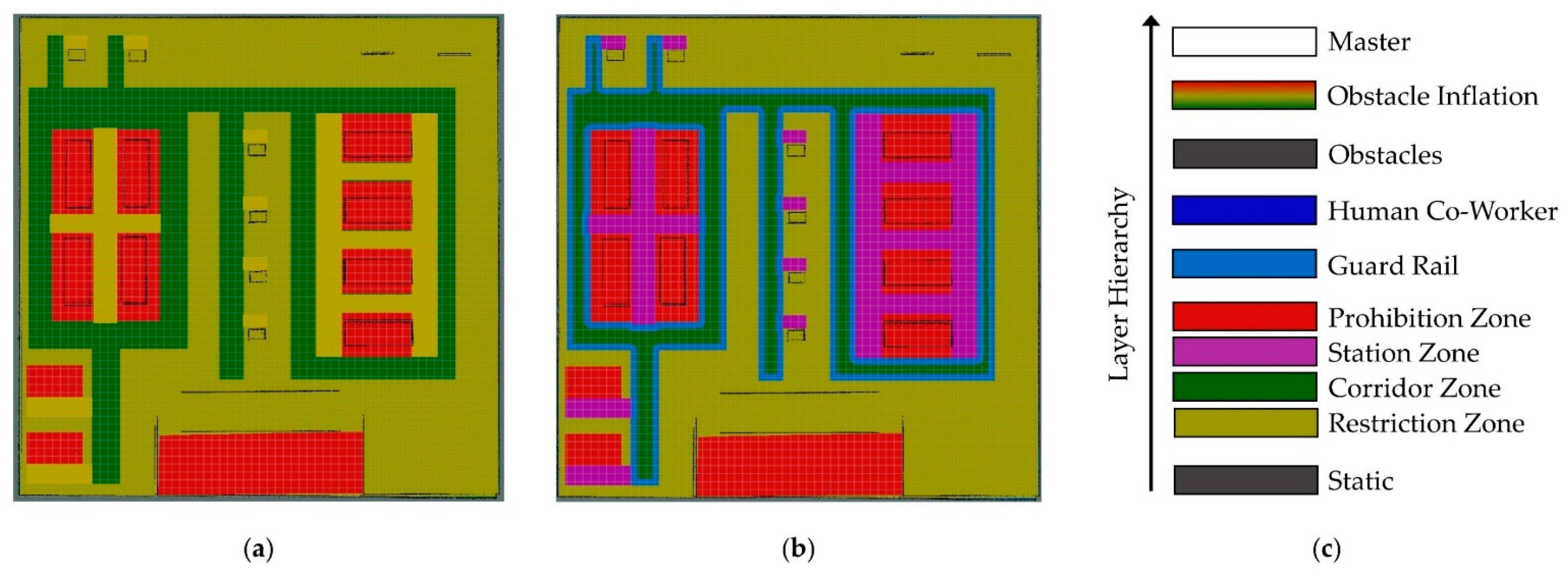
For instance, Figure 3a shows a zone-based segmentation of a 60 × 60 m production environment. The coloring represents the different cost levels of the zones ranging from green (minimum cost value) to red (maximum cost value). In Figure 3b, the zones are colored with an individual color for each zone. Figure 3c shows the corresponding layered costmap [31] configuration in hierarchical order. The ordering of the layers allows modulating the costs by overwriting them only when and where required.

The standard configuration of a layered costmap configuration includes a static, an obstacle, and an obstacle inflation layer. This default configuration does not fulfil the requirements of a dynamic production environment, including different manufacturing and transportation zones as well as a shared human–robot workspace. The implemented approach is based on the concept of layered costmaps described in [32], whereby each layer tracks the data to a specific functionality. With the cost value ${\Omega }_{xy}^i=\left\{0,1, \dots , 254, 255\right\}$ for a cell $c_{xy}^i$ at position $P_j^c=\left(x_j,y_j\right)$, the layer $i$ contributes to the Master costmap as follows:

The Static layer contributes to the master costmap by analyzing an a priori created 2D occupancy grid map $G$. The layer provides information about free and occupied spaces in the production environment by Equation (1):

$${\Omega }_{xy}^1=\{\begin{array}{c}0, G\left(x,y\right)==Free \\ 254, G\left(x,y\right)==Occupied\\ 255, G\left(x,y\right)==NoInformation \end{array}$$

(1)

with Free, Occupied, and NoInformation reflecting the related values of the occupancy grid map implementation.

The Zone layers, Corridor (2), Restricted (3), Station (4), and Prohibition (5), contribute to the zone-based navigation layout of the production environment. The dimensions of the zones are provided in form of a polygon list. The corridor zone should be the preferred zone for the implemented path planner; therefore, the cost value of the corresponding cells is set to a small value of ${\Omega }_{xy}^2=10$. The robot is allowed to enter restriction zones, but only if necessary. Therefore, the cost value for the corresponding cells is set to ${\Omega }_{xy}^3=100$. The same condition applies to the station zones. Since a motion of the robot through a restriction zone is from higher preference than a motion through a station zone, the cost value of the corresponding cells is set to ${\Omega }_{xy}^4=120$. The robot is not allowed to enter a prohibition zone; therefore, the cost value of the corresponding cells is set to ${\Omega }_{xy}^5=250$.

The Guard Rail layer is based on the inflation layer described in [32]. Originally, the inflation layer was designed to create a buffer zone around lethal obstacles to avoid the robot coming too close to the obstacles. We applied that method to define a buffer zone at the borders of the corridor zones. The robot uses these guard rail zones as a guide for navigating inside the corridor zones. The robot will navigate with a high preference alongside the edge between the guard rail zone and the corridor zone. The developed method is further explained in Section 2.2. The inflation radius is adjustable and defines the width of the guard rail zone. The corresponding cells are set to the cost value ${\Omega }_{xy}^6=12$.

The Human layer contributes the information of a multilayer and redundant workspace monitoring system (WMS) described in [29]. The WMS uses RGB and thermal images as well as Lidar data. The multilayer sensor setup is improved by the implementation of redundant algorithms for human co-worker detection based on neural networks. The fused confidence intervals between 0 and 1 are provided as a 2D heatmap in form of an occupancy grid map. The corresponding cells in the costmap $M$ are called human cells and assigned with the cost value ${\Omega }_{xy}^7=200$. A threshold of 0.5 is used for the confidence level to neglect low confidence detections. An area with an adjustable radius around each human cell is defined as a human safety zone. The Human layer calculates the Euclidean distance between the current robot position and each human cell to determine if the robot is inside a human safety zone. Following the concept of the navigation zones, the robot will preventively change its motion behavior if it is inside a human safety zone. In addition, the human cells are inflated to create a buffer zone around the human co-workers. The radius of these buffer zones is smaller compared to the human safety zones. The cost value of the corresponding cells is set to ${\Omega }_{xy}^7=200$. Theoretically, the robot is allowed to plan close to a human, but it is highly cost inefficient. Figure 4 shows an exemplary scenario of an occupancy grid map provided by the WMS and the resulting costmap, including the buffer zones in blue and one visualized human safety zone in red.

The Obstacle layer tracks the data from the 2D Lidar sensors. The Lidar data is provided in form of an array $S$, including the sensor readings. The sensor readings are converted into the costmap space to determine the corresponding cells. Analog to the Static layer, the obstacle layer contributes to the master layer by following Equation (2).

$${\Omega }_{xy}^8=\{\begin{array}{c}0, M_{Lidar}\left(x,y\right)==Free \\ 254, M_{Lidar}\left(x,y\right)==Occupied\\ 255, M_{Lidar}\left(x,y\right)==NoInformation \end{array},$$

(2)

where $M_{Lidar}$ is the sensor readings in the costmap space. The Obstacle Inflation layer adds an adjustable buffer zone around the obstacle. Therefore, the distance between the obstacle and the planned path is increased.

2.2. Cost Adaption Based on Search Expansion Direction

Common industrial navigation concepts are based on line following strategies [33] using passive [34] or active [35] landmark detection. These methods are approved in industrial environments, but not as flexible as desired. The well-known planning algorithms A* [36] or Dijkstra [37] provide the most cost-efficient path available from a start position to a goal position, given a costmap. The presented navigation concept segments the production environment in zones of different cost levels. The resulting costmap is provided to the path planner, resulting in a high preference for the corridor zone, without limiting the robot in the manner of a line follower. However, a line follower behavior is socially desirable for the corridor zone. This is particularly true for a shared human–robot production environment. In [38], the cell costs were slightly reduced for cells on the right side of a corridor. As a result, the pass speed of the human and the robot was significantly increased which indicates an optimized human–robot collaboration. The social behavior of right or left driving is widely used in public and industrial environments. Such a predictable and intuitive behavior of the robot is a key feature for beneficial human–robot cooperation.

Instead of manipulating the costs before the actual planning process, our approach is applied while planning and takes the expansion direction of the planning algorithm into concern. As a result, the desired left or right driving behavior can be applied to any zone and in any direction. The aim is that the global planner prefers a path right next to the previously mentioned guard rail zone. This behavior is comparable to a line follower, without limiting the robot to a particular line motion. Figure 5 shows a horizontal and a vertical example scenario of a planning procedure in a grid-based costmap.

The start cell for the planning procedure is set to the middle of the corridor zone. During the search for a valid path, a check is performed for each expanded cell of the corridor zone; if the cell is a neighbor of the guard rail zone, the cell is called a cell of interest. Each cell of interest can be either declared as a left-hand or right-hand driving cell. The cell type is determined by taking the expansion direction of the search algorithm into concern. The expansion direction can only be determined if a neighbored cell of interest exists. In Figure 5a, the cells at positions (7,4) and (9,8) are right-hand driving cells. The expansion direction is visualized with a red arrow. The cells at positions (9,4) and (7,8) are left-hand driving cells. The cells at (8,4) and (8,8) do not feature a specific type, since they had no neighbored cell of interest when they were expanded. In Figure 5b, the cells at (5,7) and (11,5) are right-hand driving cells. The cells at (5,5) and (11,7) are left-hand driving cells, and the cells at (5,6) and (11,6) of no type.

During search expansion the path potential is stored in form of a grid-based potential map $\Phi$. The potential map $\Phi$ holds the information for each expanded cell of how much it costs to reach that cell from the start cell. Cells that are not expanded yet, are set to a clearly identifiable default value $\phi$. Algorithm 1 shows our approach applied to realize a right-hand driving behavior.

Algorithm 1. Calculation of Potential Map for right-hand Driving
1:	function calculateCellPotential(cell $c$, costmap $M$, potential_map $\Phi$)
2:	if $c$ is not inside the corridor zone then
3:	$\Phi \left(c.x, c.y\right)=$ calculateCostsToReachCell($c$, $M$, $\Phi$)
4:	end if
5:	if$M\left(c.x,c.y-1\right)$ equal cost of GuardRailZone and $\Phi \left(c.x+1, c.y\right)$ not equal $\phi$ then
6:	$\Phi \left(c.x, c.y\right)=\Phi \left(c.x+1, c.y\right)+corridor\_cell\_cost/4$
7:	else if$M\left(c.x,c.y+1\right)$ equal cost of GuardRailZone and $\Phi \left(c.x-1, c.y\right)$ not equal $\phi$ then
8:	$\Phi \left(c.x, c.y\right)=\Phi \left(c.x-1, c.y\right)+corridor\_cell\_cost/4$
9:	else if$M\left(c.x-1,c.y\right)$ equal cost of GuardRailZone and $\Phi \left(c.x, c.y-1\right)$ not equal $\phi$ then
10:	$\Phi \left(c.x, c.y\right)=\Phi \left(c.x, c.y-1\right)+corridor\_cell\_cost/4$
11:	else if$M\left(c.x+1,c.y\right)$ equal cost of GuardRailZone and $\Phi \left(c.x, c.y+1\right)$ not equal $\phi$ then
12:	$\Phi \left(c.x, c.y\right)=\Phi \left(c.x, c.y+1\right)+corridor\_cell\_cost/4$
13:	else
14:	$\Phi \left(c.x, c.y\right)=$ calculateCostsToReachCell($c$, $M$, $\Phi$)
14:	end if
15:	end function

In this example, the right-hand driving behavior is applied to the corridor zone. The function calculateCostsToReachCell symbolizes the standard calculation of an expanded cell in the potential map, as shown in Equation (3):

$$potential=\Phi \left(c_{prev}.x,c_{prev}.y\right)+M\left(c_{exp}.x, c_{exp}.y\right)+{\Omega }_{mv},$$

(3)

where $c_{exp}$ is the expanded cell, $c_{prev}$ is the previous cell, and ${\Omega }_{mv}$ is the cost value to move from one cell to a neighboring cell. The function is triggered in case the expanded cell is not part of the corridor zone or the expanded cell is not determined as a right-hand driving cell. Therefore, in these cases, the default behaviors of the global planners are not changed.

If the expanded cell is part of a corridor zone and neighbors a guard rail zone, the cell is of interest and further analyzed. Four cases are differentiated:

• The guard rail zone is a neighbor in the negative y-direction in the costmap;
• The guard rail zone is a neighbor in the positive y-direction in the costmap;
• The guard rail zone is a neighbor in the negative x-direction in the costmap; or
• The guard rail zone is a neighbor in the positive x-direction in the costmap.

Depending on the relative position of the expanded cell in relation to the guard rail zone and the already expanded cells stored in the potential $P$, the cell is defined as a right-hand driving cell. In the case of a right-hand driving cell, the calculation of the cell potential is changed from Equation (3). The applied formula is shown in Equation (4):

$$potential=\Phi \left(x_i,y_i\right)+M_{Corridor} / 4$$

(4)

The coordinates $x_i,y_i$, with $i=\left\{1,2,3,4\right\}$, reflect the above mentioned four cases. $M_{Corridor}$ is the cost value of a cell inside the corridor zone.

The presented approach can be applied to any zone in any direction, as long as a particular cost gradient is present between the zone and the guard rail zone. Figure 6 shows an example scenario for a large-scale planning scenario in a simulated production environment. The red dot represents the start position and the green dot the goal position. The costmap is divided into navigation zones according to Section 2.1. Figure 6a shows the default behavior of the implemented A* planner. As desired, the resulting path is mostly located inside the corridor zone. Figure 6b shows the resulting right driving behavior by applying our approach.

2.3. Large-Scale Surface Orthogonal Motion Planning

The addressed inspection task requires a high positioning accuracy of the radar module (<200 µm) in reference to the workpiece frame for each scan process. Therefore, the large-scale inspection task is executed in asynchronous mobile manipulation mode. The workpiece is divided into smaller subsegments, which can be inspected standalone with the motion capabilities of the manipulator. At each subsegment, the following process steps are performed:

• Surface reconstruction;
• Sensor waypoint generation;
• Motion planning.

The approached positions of the mobile platform are determined by analyzing the reachability of the manipulator in its workspace and segmenting the workpiece accordingly.

2.3.1. Surface Reconstruction

To plan a path on a surface, the geometrical shape of the surface must be known. Especially for inspection tasks, it cannot be assumed that the actual state of the workpiece still corresponds to its computer-aided design (CAD) data. In our implementation, the surface is reconstructed from a point cloud using the Point Cloud Library [39] (PCL). The point cloud is provided by the RGB-D camera at the end effector of the manipulator. In the first step, the point cloud is down-sampled, and then the surface is reconstructed by applying B-spline fitting [40]. Figure 7 shows the reconstructed surface of an exemplary rotor blade segment.

2.3.2. Waypoint Generation

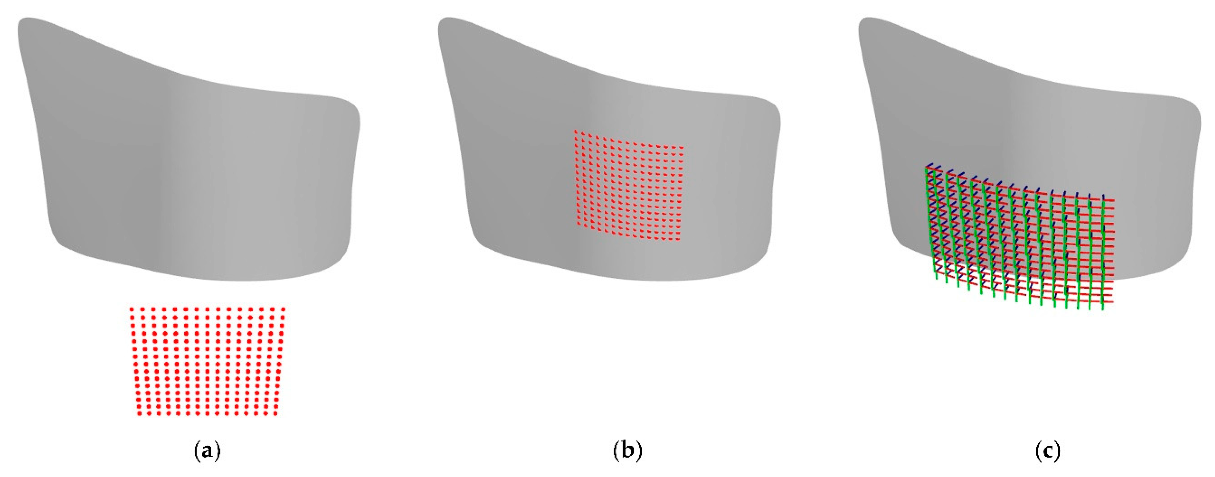
The surface orthogonal motion planning is inspired by the approach presented in [41], which addresses an inspection task of a landscape with an unmanned aerial vehicle (UAV). For this purpose, the landscape is rasterized into a grid. The grid resolution depends on the technical parameters of the sensor, the desired image resolution, and the desired overlaps of the individual images. The centers of the grid cells are shifted along the normal of the ground surface. This approach was adapted for the creation of 6D waypoints, representing surface orthogonal 6D poses of the radar sensor. Figure 8 shows the three steps of the implemented waypoint generation method, applied to the reconstructed surface of Figure 7. Figure 8a shows the centers of the grid cells. These are projected onto the reconstructed surface (see Figure 8b). The projected centers are shifted along the surface normal to the desired distance from the surface. The z-axis of the 6D waypoints are aligned with the negative surface normals (see Figure 8c).

2.3.3. Path Planning

The 6D waypoints can be considered as nodes in a complete graph. A Hamiltonian cycle [42] in this graph visits all waypoints. The search for the shortest Hamiltonian cycle in a complete and weighted graph is called the traveling salesman problem (TSP). This problem is NP-complete, and there is no known efficient algorithm to solve it [43]. One approximation approach is the algorithm according to Christofides [44]. The implemented approach is shown in Algorithm 2.

Algorithm 2. Factor 3/2 approximation of the travelling salesman problem
1:	function approximateTSP(Graph $G$, costfunction $\omega$)
2:	choose a root node $r ϵ V\left(G\right)$ as base v
3:	calculate the minimum spanning tree $T$ for $G$ with $MST-Prim\left(G,\omega , r\right)$
4:	calculate the perfect matching with minimum weight $m$ for odd $v ϵ V\left(G\right)$
5:	add $E\left(m\right)$ to $T$
6:	determine the Euler cycle $\Gamma$ in $m+T$
7:	the Hamiltonian cycle $H$ is the ordered list of nodes visited on $\Gamma$, multiple nodes are skipped
8:	return $H$
9:	end function

The path length is limited to a maximum of one and a half times the optimal solution. The algorithm first calculates a minimum spanning tree [43] (MST). A minimum perfect match is formed between the nodes of the MST with an odd degree. This is possible because there is always an even number of nodes with an odd degree. In the path planning implementation, the Blossom-V implementation from [45] is used for this purpose. The edges of the matching are added to the MST, such that the degree of all nodes is even. Thus, a Euler cycle can be formed in the graph. By truncation, i.e., deleting multiple visited nodes, the approximate solution of the TSP is formed.

2.3.4. Positioning of the Mobile Platform

The mobile platform must be positioned in such a way that the surface orthogonal planned path of the end effector lies in a workspace region with high reachability. The method used to determine the characteristics of the manipulator’s workspace is described in [29]. The size of the chosen suitable area of the manipulator workspace directly affects the segmentation of the workpiece in local subsegments.

The workpiece segmentation consists of the following steps:

• Create the scanning grid accordingly to the workpiece size (see Figure 9a);
• Project the scanning grid onto the surface of the workpiece (see Figure 9b);
• Reflect the projected points alongside the surface normal (see Figure 9c); and
• Cluster the reflected points into processable local scan areas (see Figure 9d).

The reflected points represent positions of the manipulator’s end-effector. The aim of the workpiece segmentation is to find a set of neighbored projected points, whereby the corresponding reflected points are inside the defined workspace of the manipulator. Therefore, a list of position tuples ${\mathsf{\Lambda }}_{PR}$ is created, whereby each tuple consists of a projected point and the corresponding reflected point. By continuously expanding in the domain of the projected points and checking the reachability of the corresponding reflected points, the tuples of list ${\mathsf{\Lambda }}_{PR}$ are clustered into suitable local scan areas. The implemented method is described in detail in Algorithm 3.

Algorithm 3. Segmentation of the workpiece into subsegments
1:	function segmentWorkpiece(CADModel $\Psi$, Workspace ${\rm Y}$, Distance $d$, ClusterList ${\mathsf{\Lambda }}_{PR}$)
2:	create sampling grid $S$ accordingly to 3D bounding box size of $\Psi$
3:	project grid points $s_i ϵ S$ onto surface of $\Psi$
4:	reflect projected points alongside the corresponding surface normal to distance $d$ from surface of $\Psi$
5:	create a list $L_{PR}$ with corresponding pairs of projected and reflected points
6:	ascendingly order $L_{PR}$ based on Euclidean distance between projected point and workpiece frame $I$
7:	while $L_{PR}$ not empty do
8:	initialize empty cluster $C_{PR}$
9:	add position pair at first position of $L_{PR}$ to $C_{PR}$ and remove pair from $L_{PR}$
11:	initialize filter dimensions
12:	set current search direction to $I_x$-direction
13:	while not all search directions are exhausted do
14:	extend filter in search direction
15:	if filter dimension is beyond the bounding box of $\Psi$ then
16:	mark current search direction as exhausted
17:	reset filter dimensions
18:	end if
19:	find all position pairs ${Л}_i$ in $L_{PR}$ where the reflected point is inside filter bounds
20:	calculate bounding box dimension $B$ of all reflected points ϵ ${Л}_i$
21:	if $B\subseteq {\rm Y}$ then
22:	add ${Л}_i$ to $C_{PR}$ and delete ${Л}_i$ from $L_{PR}$
23:	else
24:	reset filter dimension
25:	mark search direction as exhausted
26:	end if
27:	switch search direction
28:	end while
29:	add $C_{PR}$ to ${\mathsf{\Lambda }}_{PR}$
30:	end while
31:	end function

The mobile platform is positioned in such a way that the center of the calculated scan area $l_i={\left(x_I,y_I\right)}^T$ is located at the center of the system’s reachable workspace $r_i={\left(x_R,y_R\right)}^T$. Therefore, the centers $c_i$ are translated alongside the x-axes of the workpiece coordinate system $I$. Depending on the approach direction of the mobile platform, the translation is performed in $x^{+}$- or $x^{-}$-direction. The shifted positions $l_i^{*}$ are converted into 2D poses $L_i={\left(x_I,y_I,{\theta }_I\right)}^T$ by adding an orientation accordingly to the translation direction. The 2D poses are transformed into the world coordinate system $W$, resulting in the required 2D goal poses for the navigation task.

2.4. Task Management

The inspection of a large-scale rotor blade is a long-running task. Therefore, we designed a task management system in form of a nested state machine. The state machine uses the SMACH framework [46]. The main state machine includes two nested state machines managing the manipulation and the navigation task. Figure 10 shows the task management system.

The main state machine requires as input the model of the workpiece (CAD File), the desired distance between the radar sensor and the surface of the workpiece (Distance_SR) and the characteristics of the used manipulator (Manipulator_Info). The Manipulator_Info consists of the suitable area of the manipulator workspace, including the corresponding maximum reach of the manipulator.

The workpiece segmentation and the position determination of the platform at the local scan subsegments is executed a priori. The workpiece segmentation provides the local scan areas (ScanAreas_Info). Each ScanArea_Info consists of the area center (ScanArea_Center) and the dimensions (ScanArea_Dim) in reference to the workpiece coordinate system. The platform positioning converts the centers of the local scan areas into 2D navigation goals (Poses_Goal) in reference to the world coordinate system.

The navigation and manipulation state machines are triggered sequentially for each pair of navigation goal (Pose_Goal) and local scan area (ScanArea_Dim). The navigation state machine takes care about the path planning and path execution processes. The move base flex [47] framework is implemented to change between different motion behaviors of the mobile platform depending on the current navigation zone. The manipulation state machine is divided into three process steps. The point cloud executor gathers the point cloud data at the local scan pose (Pose_Scan) and crops it accordingly to the dimensions of the local scan area. The waypoint generator determines the 6D end-effector waypoints (Waypoints_EE), orthogonal oriented to the surface of the workpiece. The manipulation executor controls the motion of the manipulator.

3. Experiments and Discussions

3.1. Production Environment Navigation

We evaluated the presented zone-based navigation concept in the multi-robot simulator Gazebo [48]. Therefore, we created 10 different production environments of the size 60 × 60 m. Each simulated production environment features an individual navigation zone layout, comparable to the layout shown in Figure 6. In each simulated production environment, we defined 10 start-goal-position tuples, which resulted in a total of 100 tuples. The tuples were divided into five groups:

• Tuples $T_{RR}$ from restricted-to-restricted zone;
• Tuples $T_{SS}$ from station-to-station zone;
• Tuples $T_{SC}$ from station-to-corridor zone;
• Tuples $T_{CS}$ from corridor-to-station zone;
• Tuples $T_{CC}$ from corridor-to-corridor zone.

The five groups are equally distributed across the 10 simulated environments, resulting in two tuples for each group per environment.

For each tuple, we manually annotated the desired path $P_i$ with $i=\left\{1,2,\dots ,100\right\}$. Each path $P_i$ fulfills two criteria. The first one is the reduction in the overall costs of the path by preferring the corridor zone. The second one respects the desired right-hand driving behavior alongside the corner between the corridor zone and the guard rail zone.

The experiment compares the performance of the default A* and Dijkstra implementation of the robot operating system (ROS) [49] with our adapted version, later called A*_zone and Dijkstra_zone.

The deviation between a planned path $A$ and the corresponding manually annotated path $B ϵ P_i$ is represented by the average mean square error $aMSE$. The calculation is given in Equation (5):

$$aMSE=\frac{{{\displaystyle \sum }}_{i=0}^n{d}_i^2}{n},$$

(5)

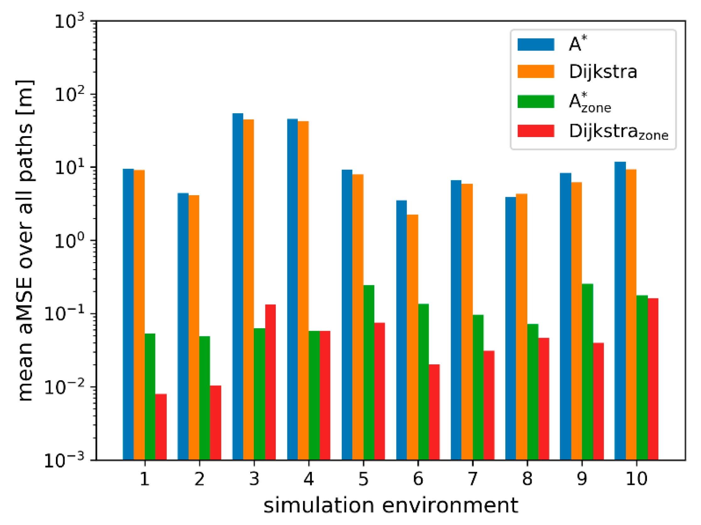
where $d_i$ is the Euclidean distance between each of the $n$ positions $a_i ϵ A$ and its closest neighbored position $b_i ϵ B$. Figure 11 shows the experimentally determined results for each of the 10 simulated production environments averaged over all five start-goal-position tuple groups.

As expected, the $aMSE$ is significantly higher for the default implementations of A* and Dijkstra. This result is caused by the right-hand driving criteria of the manually annotated reference paths. In addition to the $aMSE$, we analyzed the following performance parameters:

• The required process time;
• The number of expanded cells; and
• The path length.

The required process time indicates the additional computation effort caused by the implementation of Algorithm 1. The number of expanded cells reflects the efficiency of reaching the goal cell. The overall path length shows the additional path caused by the desired right driving behavior.

Table 1. Comparison of the evaluated planning approaches. Performance parameters averaged over 100 start-goal-position tuples in 10 simulated environments.

Approach	aMSE [m]	Processing Time [ms]	Expanded Cells	Path Length [m]
A*	15.72	56.2	401,497	62.43
Dijkstra	13.78	53.3	596,325	62.22
A*zone	0.11	49.8	355,200	71.04
Dijkstrazone	0.06	49.1	545,255	72.84

shows the performance parameters averaged over all 100 start-goal-position tuples.

The default implementations of A* and Dijkstra provide the most cost-efficient path. The cost efficiency is mainly influenced by the cost levels of the different zones. Inside a zone, the length of the path is the factor of influence. Therefore, the average path length of the default implementations is approximately 14% smaller compared to our approach. With an average $aMSE$ of 0.11 m for A*_zone and 0.06 m for Dijkstra_zone, our approach proved to provide consistent paths following the concept of right-hand driving.

The general difference in processing time between the approaches A*, A*_zone and Dijkstra, and Dijkstra_zone is caused by the calculation of the heuristic. Therefore, the average processing time for A*_zone is 2.5% greater than that for Dijkstra_zone, even though the number of expanded cells is approximately 35% smaller.

The additional computation effort needed to determine the right-hand driving cells at each expansion step does not increase the overall processing time. Quite the opposite, the approach A*_zone needs approximately 11% less average processing time. This decrease correlates with the number of expanded cells, which is also approximately 11% smaller than that of A*. The same applies to the approach Djikstra_zone, which results in 9% less expanded cells and a corresponding decrease in the overall processing time.

Table 2. The number of expanded cells normalized to the path length.

Approach	${\mathit{T}}_{\mathit{R}\mathit{R}}$	${\mathit{T}}_{\mathit{S}\mathit{S}}$	${\mathit{T}}_{\mathit{S}\mathit{C}}$	${\mathit{T}}_{\mathit{C}\mathit{S}}$	${\mathit{T}}_{\mathit{C}\mathit{C}}$
A*	7643	9801	2836	8852	3298
Dijkstra	10,366	11,294	6261	11,663	6425
A*zone	6170	7745	1695	7963	1623
Dijkstrazone	8219	8818	4401	10,115	4496

shows a comparison of the five start-goal-position tuple groups by evaluating the number of expanded cells normalized to the resulting path length for each tuple.

The goal zone has a high impact on the efficiency of the evaluated path planners. If the goal position lies within the corridor zone ($T_{SC}$, $T_{CC}$), the number of expanded cells is significantly lower compared to a goal position outside the corridor zone ($T_{RR}$, $T_{SS}, T_{CS}$), by comparing columns $T_{SC}$, $T_{CC}$ with other columns of Table 2. This behavior is caused by the cost levels of the zones and the nature of the path planning algorithms. Since the cost level of the corridor zone is relatively low the planners will expand inside the corridor zone with a high preference, before starting to expand inside a restricted or station zone. The A* and A*_Zone implementations provide a lower number of expanded cells for each paths group, as highlighted by the bold font in Table 2, which is caused by the additional heuristic.

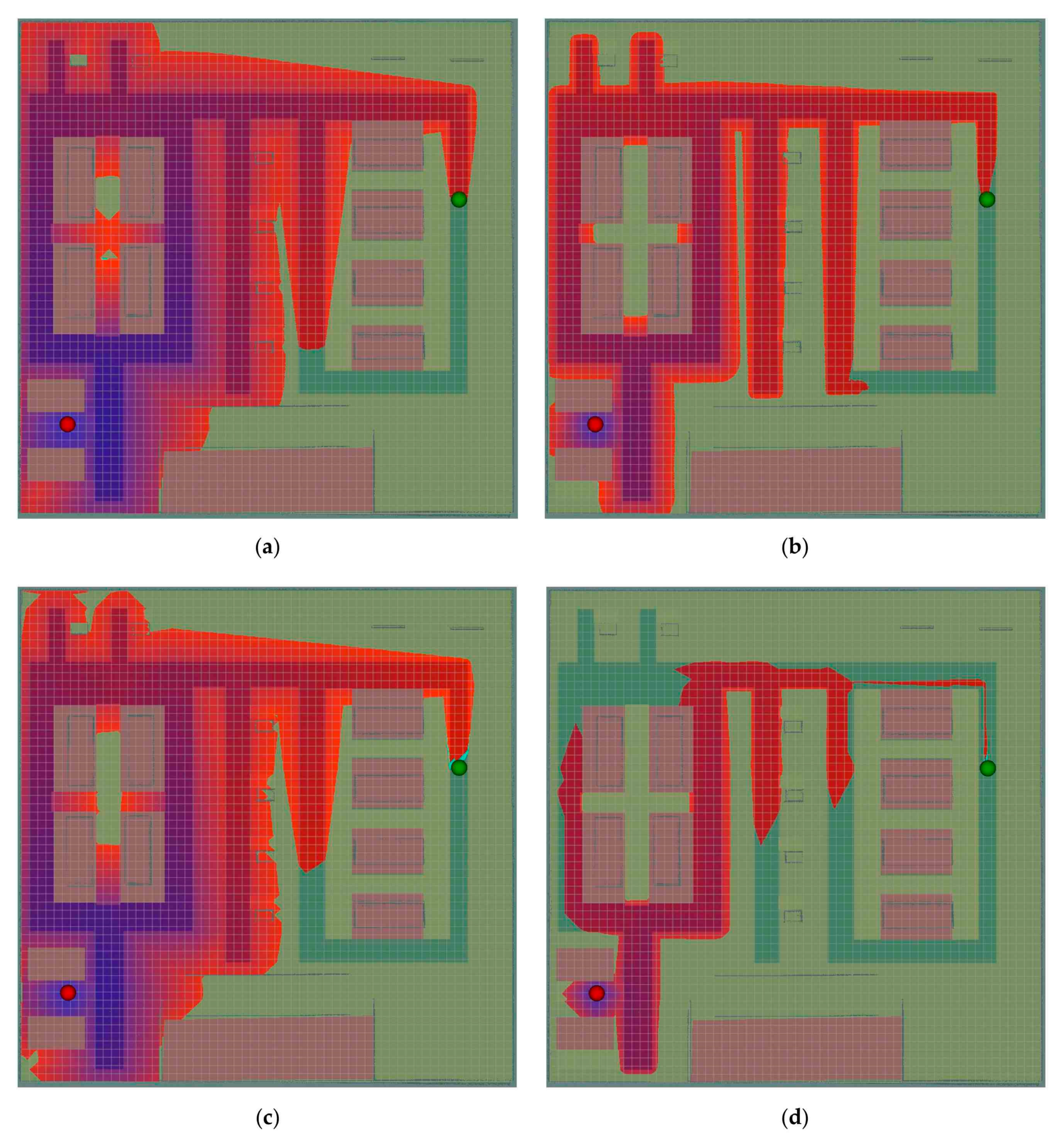
Our right-hand driving approach results in an additional decrease in the number of expanded cells. This is caused by the effect of our method on the behavior of the path planning algorithms. Figure 12 shows a comparison of a path $p\in T_{SC}$ and the corresponding expansion potentials for each of the evaluated approaches.

The relatively low-cost cells at the edge between the corridor zone and the guard rail zone let the path planning algorithms concentrate their expansion towards a particular direction. Since the corridor zone is designed to connect typical station areas in the industrial environment, our method reduces the number of cells that are expanded in the corridor zone. Therefore, our method provides a higher expansion efficiency which results in lower computational effort compared to standard implementations of Dijkstra or A*.

3.2. Evaluation in Real-World Use-Case

The presented concept is evaluated at a typical rotor blade form, which features a length of 11 m. Due to space limitations of the experiment environment, only the tip of the form is used throughout the experiment. Figure 13a shows the 3D model of the tip. The tip has the dimensions 2.0 × 0.8 × 0.9 m³ (LxHxW). Figure 13b,c show the real-world form equipped with glass fiber mats and a setup for vacuum generation.

Figure 14a shows the analyzed workspace of the used Universal Robot UR5 displayed as a cut in the x, y-plane of the manipulator coordinate frame $R$. Since the end-effector will be downward oriented most of the time during inspection and accordingly to [29], the used geometric primitive to analyze the workspace is a downward facing hemisphere. Each analyzed voxel has the edge length of 50 mm. Figure 14b shows the same cut, with a threshold at 50% reachability applied.

The chosen suitable workspace area consists of two layers in z-direction to cover the curved shape of the blade tip form. The area is shown in Figure 14c and of size: 0.45 m in x-direction, 0.7 m in y-direction, and 0.1 m in z-direction of the coordinate system $R$.

In addition, the so-called max reach value $ma{x}_{reach}$ of the mobile manipulator is calculated. The $ma{x}_{reach}$ symbolizes the maximum distance the manipulator is able to reach into the workpiece alongside the robot coordinate system $R$. The calculation is given in Equation (6):

$$ma{x}_{reach}=D_{MW}-\left(d_{RPF}+d_{PFW}\right),$$

(6)

where $D_{MW}$ is the distance between the origin of $R$ and the reachable voxel, which is located at the maximum distance alongside the x-axis of $R$. The distances $d_{RPF}$ and $d_{PFW}$ depend on the hardware setup and the minimum safety distance between the platform and the workpiece. The distance $d_{RPF}$ describes the distance between the origin of $R$ and the front of the mobile platform. The distance $d_{PFW}$ describes the safety distance between the front of the mobile platform and the workpiece.

Based on the method presented in Section 2.3.4, the workpiece is segmented in inspectable subsegments taking the maximum reach $ma{x}_{reach}$ of the hardware setup into account. Figure 15a shows the colored subsegments. Figure 15b shows the corresponding poses of the mobile platform as black arrows for each subsegment. Figure 15c shows the mobile manipulator executing the scan process at a subsegment of the work piece.

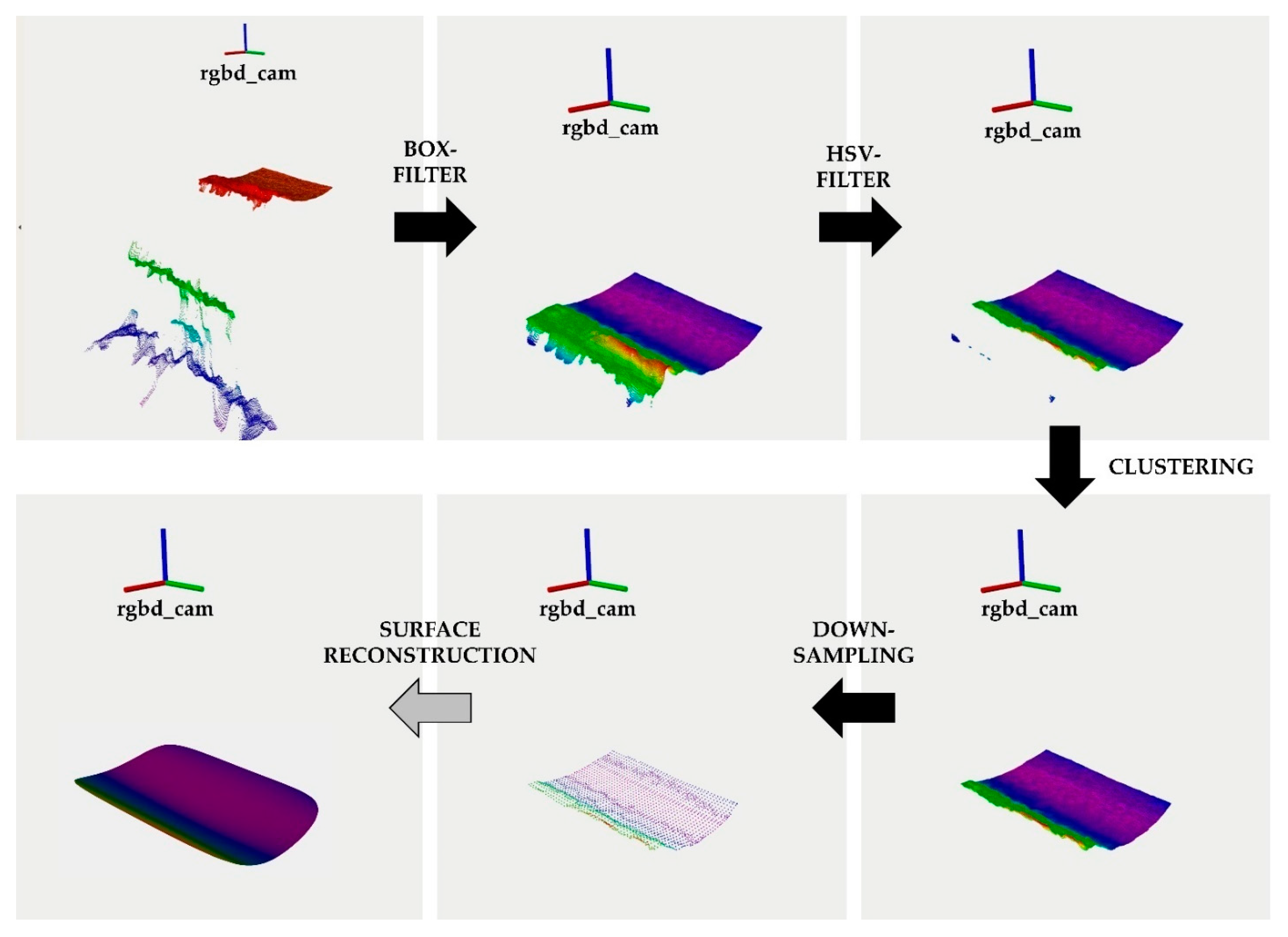
At each local subsegment, the surface reconstruction (cf. Section 2.3.1) is executed. Therefore, an RGB-D camera provides a point cloud of the work piece. A crop box filter removes all points, which are related to the ground or the robot itself. In the next step, a HSV filter is applied to the remaining points to remove points related to the yellow corner tape of the vacuum setup (cf. Figure 15c). The resulting point are clustered by their Euclidean distance to determine the points belonging to the scanning surface. A down sampled version of the resulting point cloud is used for the surface reconstruction. Figure 16 shows the complete pipeline for a point cloud captured at a local subsegment.

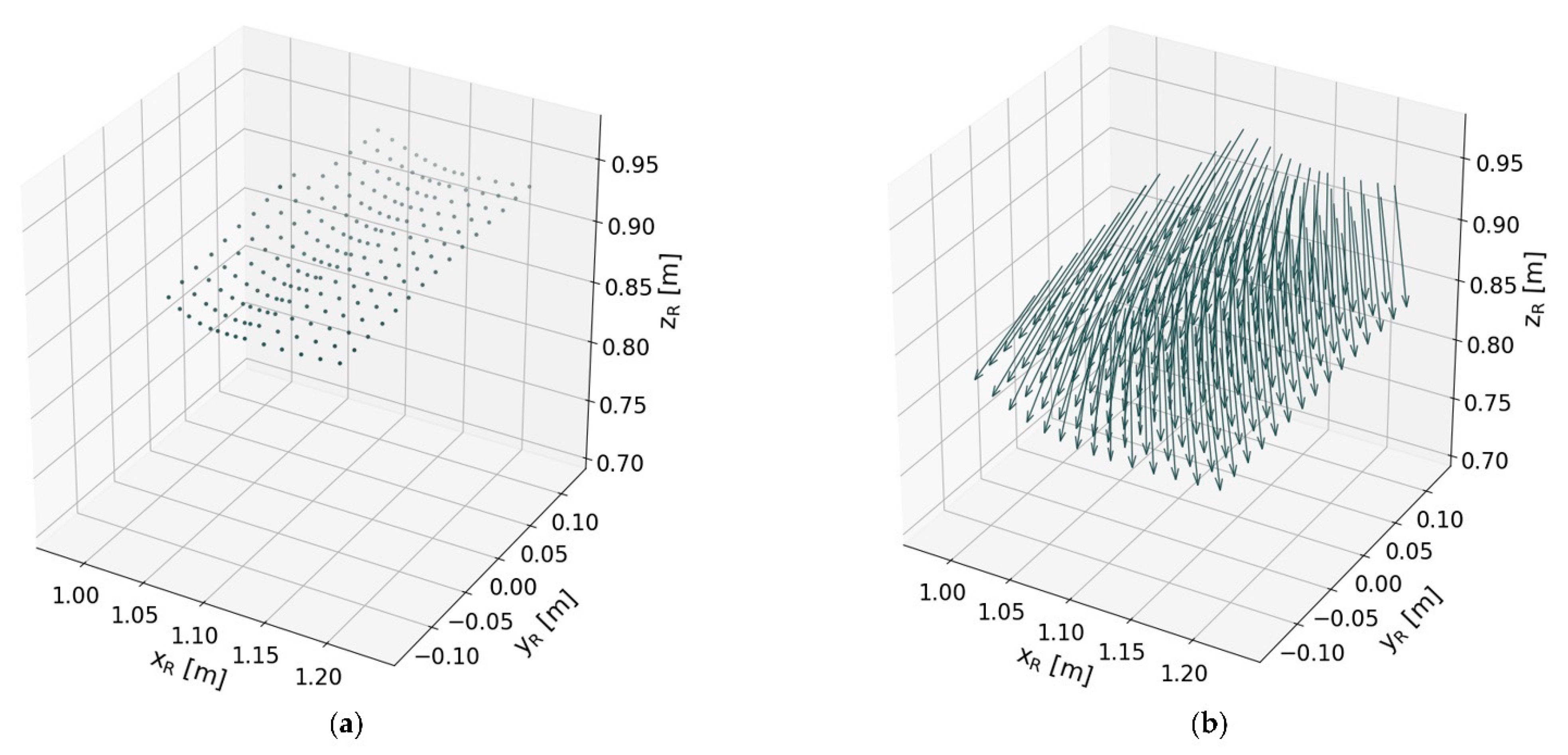
The waypoint generation (cf. Section 2.3.2) is based on the surface reconstruction. Figure 17a shows the approached 3D positions of the end-effector in the robot coordinate frame $R$ during the inspection process of one local subsegment. Figure 17b shows the surface-orthogonal orientation of the end-effector at each 3D position.

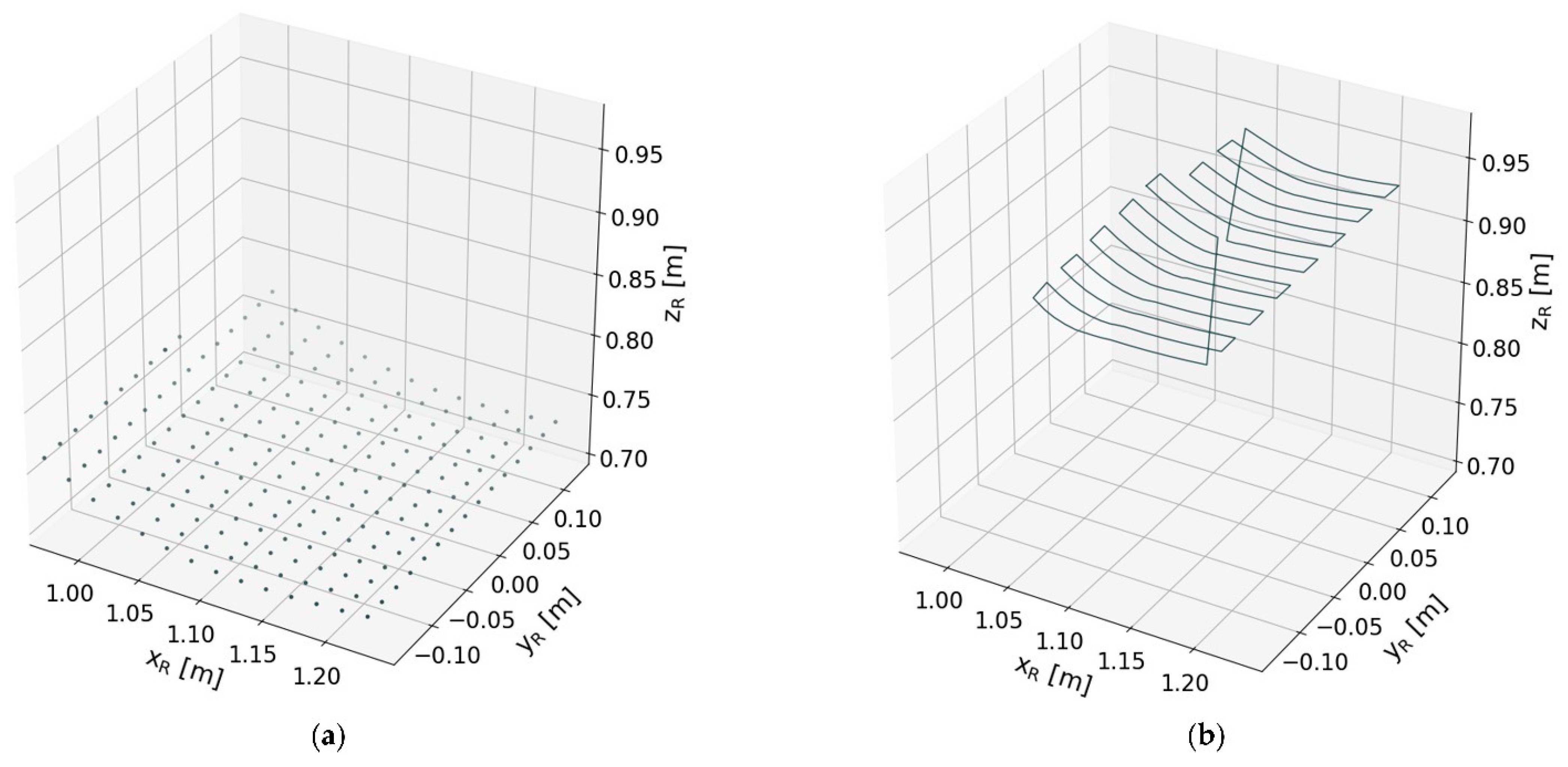
The 3D positions of the end-effector are shifted alongside the calculated surface normal by the amount of the chosen scanning height. The resulting 3D positions reflect the surface of the workpiece (see Figure 18a). Figure 18b shows the path of the end-effector during the inspection process.

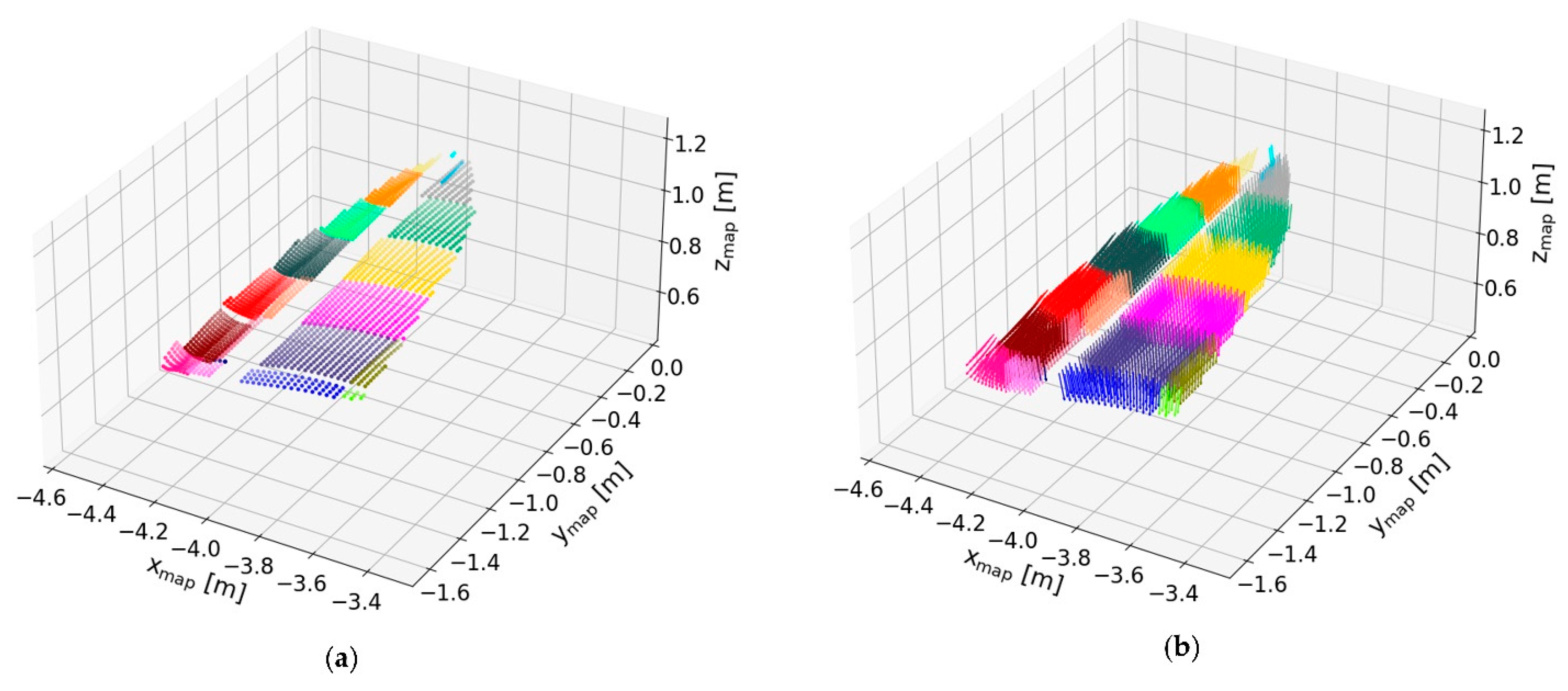
The pose information of each local subsegment is transformed into the static global frame $\mathrm{map}$. Therefore, the localization capabilities of the mobile manipulator OMNIVIL are used, as described in [29]. Figure 19a shows the approached 3D positions of the end-effector in the map frame. The positions are colored accordingly to their related local subsegment. Figure 19b shows the surface-orthogonal orientation of the end-effector at each 3D position.

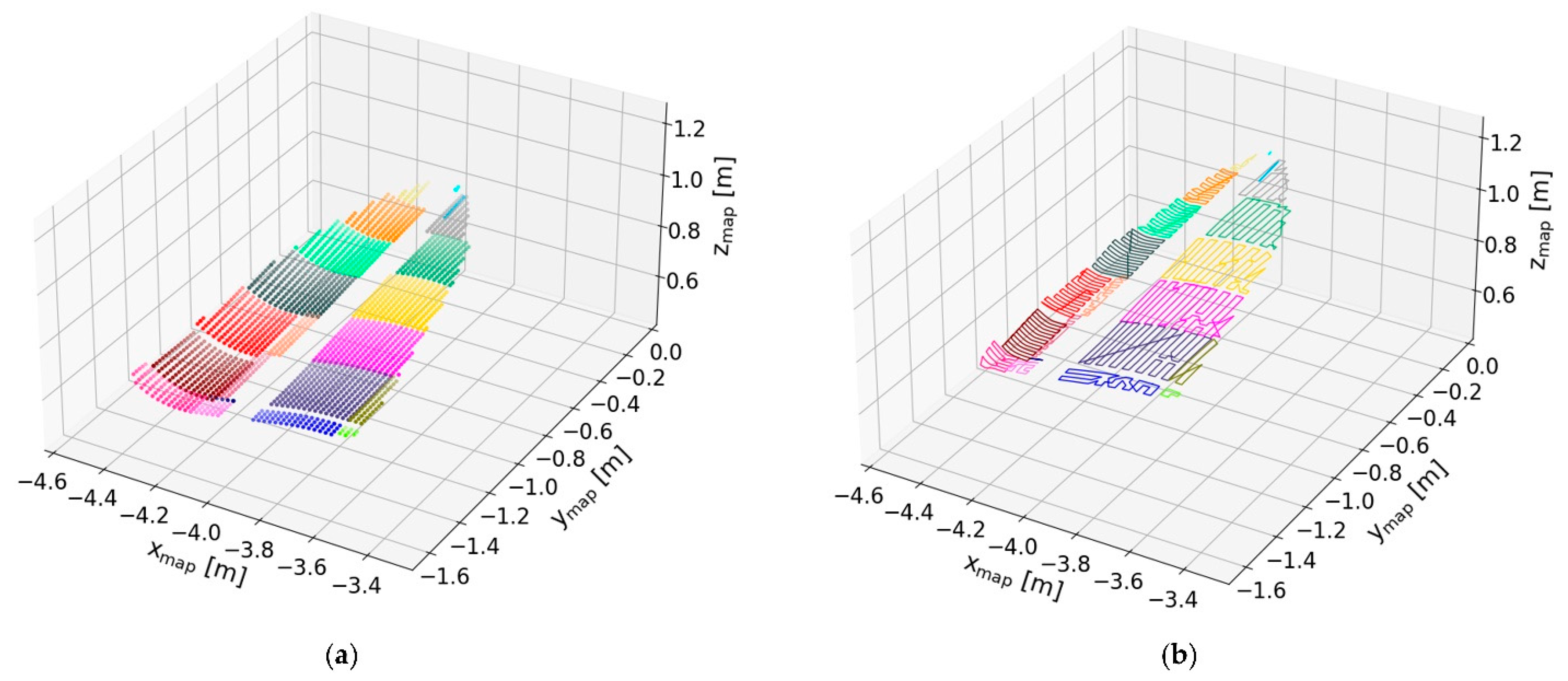
Figure 20a shows the shifted end-effector positions, which reflect the concave and convex shape of the scanned surface. The middle part of the form is not covered due to the limited maximum reach of the used manipulator UR5. Figure 20b shows the path of the end-effector executed at each local subsegment.

4. Conclusions

This study presented a method for the automation of the large-scale inspection process of wind turbine blades in manufacturing. The focus was set on the control of the autonomous mobile manipulator. It provided insights into related research fields, including autonomous navigation and surface orthogonal motion planning. The presented methods are applicable to various tasks related to large-scale inspection.

The developed approach realized autonomous navigation including a zone-based segmentation of the production environment. The common approach of a layered costmap was extended to fulfil the needs of a collaborative human–robot industrial environments. In addition, a new method was presented, which manipulates the cost values during the search expansion of a path planner. The method was applied to the state-of-the-art algorithms A* and Dijkstra and was used to realize a right-hand driving behavior of the mobile manipulator in corridor zones. An experiment in a simulation environment showed the superior efficiency and reliability of the method. The actual inspection process was performed in an asynchronous mode by the mobile manipulator. Therefore, a method was developed to segment the workpiece into smaller subsegments, which can be inspected by the manipulator. The motion planning at the local subsegments used a surface reconstruction based on point cloud data. The resulting waypoints were considered nodes in a complete graph. The problem to find the shortest path was solved by applying algorithms related to the traveling salesman problem. The developed system was evaluated in a real-use case.

Further improvements will focus on the segmentation of the production environment. The segmentation can be performed automatically by taking documentation of the factory layout into a concern or by identifying workstations by the robot itself. Furthermore, the generation of the workpiece model should be performed by the robot itself.

References

1. GWEC. Global Wind Report 2021. Available online: https://www.windenergyhamburg.com/fileadmin/windenergy/2022/pdf/we_gwec-global-wind-report-2021.pdf (accessed on 3 May 2021).
2. Ancona, D.; McVeigh, J. Wind Turbine-Materials and Manufacturing Fact Sheet; Princeton Energy Resources International, LLC: Rockville, MD, USA, 2001; p. 19. [Google Scholar]
3. Murray, R.; Swan, D.; Snowberg, D.R.; Berry, D.; Beach, R.; Rooney, S. Manufacturing a 9-Meter Thermoplastic Composite Wind Turbine Blade. In Proceedings of the American Society for Composites Thirty-Second Technical Conference, West Lafayette, IN, USA, 23–25 October 2017; DEStech Publications: Lancaster, PA, USA, 2017. ISBN 978-1-60595-418-9. [Google Scholar]
4. Yang, K.; Rongong, J.A.; Worden, K. Damage detection in a laboratory wind turbine blade using techniques of ultrasonic NDT and SHM. Strain 2018, 54, e12290. [Google Scholar] [CrossRef]
5. Garcia Marquez, F.P.; Gomez Munoz, C.Q. A new approach for fault detection, location and diagnosis by ultrasonic testing. Energies 2020, 13, 1192. [Google Scholar] [CrossRef] [Green Version]
6. Yang, R.; He, Y.; Mandelis, A.; Wang, N.; Wu, X.; Huang, S. Induction infrared thermography and thermal-wave-radar analysis for imaging inspection and diagnosis of blade composites. IEEE Trans. Ind. Inform. 2018, 14, 5637–5647. [Google Scholar] [CrossRef]
7. Hwang, S.; An, Y.-K.; Sohn, H. Continuous line laser thermography for damage imaging of rotating wind turbine blades. Procedia Eng. 2017, 188, 225–232. [Google Scholar] [CrossRef]
8. Arnold, P.; Moll, J.; Mälzer, M.; Krozer, V.; Pozdniakov, D.; Salman, R.; Rediske, S.; Scholz, M.; Friedmann, H.; Nuber, A. Radar-based structural health monitoring of wind turbine blades: The case of damage localization. Wind Energy 2018, 21, 676–680. [Google Scholar] [CrossRef]
9. Herschel, R.; Pawliczek, S. 3D millimeter wave screening of wind turbine blade segments. In Proceedings of the 15th European Radar Conference (EuRAD), Madrid, Spain, 26–28 September 2018; pp. 115–117, ISBN 2874870536. [Google Scholar]
10. Froehly, A.; Herschel, R. Refraction Compensation in Non-Destructive Testing. In Proceedings of the 15th European Conference on Antennas and Propagation (EuCAP), Düsseldorf, Germany, 22–26 March 2021; pp. 1–5, ISBN 8831299026. [Google Scholar]
11. Enevoldsen, P.; Xydis, G. Examining the trends of 35 years growth of key wind turbine components. Energy Sustain. Dev. 2019, 50, 18–26. [Google Scholar] [CrossRef]
12. Mishnaevsky, L.; Branner, K.; Petersen, H.N.; Beauson, J.; McGugan, M.; Sørensen, B.F. Materials for wind turbine blades: An overview. Materials 2017, 10, 1285. [Google Scholar] [CrossRef] [PubMed] [Green Version]
13. Hvilshøj, M.; Bøgh, S.; Nielsen, O.S.; Madsen, O. Autonomous industrial mobile manipulation (AIMM): Past, present and future. Ind. Robot Int. J. 2012, 39, 120–135. [Google Scholar] [CrossRef]
14. Schuler, J. Integration von Förder- und Handhabungseinrichtungen; Springer: Berlin, Germany, 1987. [Google Scholar]
15. Hvilshøj, M.; Bøgh, S.; Nielsen, O.S.; Madsen, O. Multiple part feeding—Real-world application for mobile manipulators. Assem. Autom. 2012, 32, 62–71. [Google Scholar] [CrossRef] [Green Version]
16. Halt, L.; Meßmer, F.; Hermann, M.; Wochinger, T.; Naumann, M.; Verl, A. AMADEUS-A robotic multipurpose solution for intralogistics. In Proceedings of the 7th German Conference on Robotics, ROBOTIK 2012, Munich, Germany, 21–22 May 2012; pp. 1–6. [Google Scholar]
17. Krueger, V.; Chazoule, A.; Crosby, M.; Lasnier, A.; Pedersen, M.R.; Rovida, F.; Nalpantidis, L.; Petrick, R.; Toscano, C.; Veiga, G. A Vertical and Cyber–Physical Integration of Cognitive Robots in Manufacturing. Proc. IEEE 2016, 104, 1114–1127. [Google Scholar] [CrossRef]
18. Bogh, S.; Schou, C.; Ruehr, T.; Kogan, Y.; Doemel, A.; Brucker, M.; Eberst, C.; Tornese, R.; Sprunk, C.; Tipaldi, G.D.; et al. Integration and Assessment of Multiple Mobile Manipulators in a Real-World Industrial Production Facility. In Proceedings of the 41st International Symposium on Robotics, Munich, Germany, 2–3 June 2014; pp. 1–8. [Google Scholar]
19. Dömel, A.; Kriegel, S.; Kaßecker, M.; Brucker, M.; Bodenmüller, T.; Suppa, M. Toward fully autonomous mobile manipulation for industrial environments. Int. J. Adv. Robot. Syst. 2017, 14, 1–19. [Google Scholar] [CrossRef] [Green Version]
20. Outón, J.L.; Villaverde, I.; Herrero, H.; Esnaola, U.; Sierra, B. Innovative Mobile Manipulator Solution for Modern Flexible Manufacturing Processes. Sensors 2019, 19, 5414. [Google Scholar] [CrossRef] [PubMed] [Green Version]
21. Saenz, J.; Vogel, C.; Penzlin, F.; Elkmann, N. Safeguarding Collaborative Mobile Manipulators—Evaluation of the VALERI Workspace Monitoring System. Procedia Manuf. 2017, 11, 47–54. [Google Scholar] [CrossRef]
22. Fritzsche, M.; Saenz, J.; Penzlin, F. A large scale tactile sensor for safe mobile robot manipulation. In Proceedings of the 11th International Conference on Human-Robot Interaction (HRI), Christchurch, New Zealand, 7–10 March 2016; pp. 427–428. [Google Scholar]
23. Andersen, R.S.; Bøgh, S.; Moeslund, T.B.; Madsen, O. Intuitive task programming of stud welding robots for ship construction. In Proceedings of the International Conference on Industrial Technology, Seville, Spain, 17–19 March 2015; pp. 3302–3307. [Google Scholar]
24. Yu, L.; Yang, E.; Ren, P.; Luo, C.; Dobie, G.; Gu, D.; Yan, X. Inspection Robots in Oil and Gas Industry: A Review of Current Solutions and Future Trends. In Proceedings of the 25th International Conference on Automation and Computing (ICAC), Lancaster, UK, 5–7 September 2019; pp. 1–6, ISBN 978-1-8613-7665-7. [Google Scholar]
25. Hashim, A.S.; Grămescu, B.; Niţu, C. State of the Art Survey on Using Robots in Oil and Gas Industry. In Proceedings of the International Conference of Mechatronics and Cyber-MixMechatronics—2017, Bucharest, Romania, 7–8 September 2017; Springer International Publishing: Cham, Switzerland, 2018; pp. 177–185. [Google Scholar]
26. Lu, S.; Zhang, Y.; Su, J. Mobile robot for power substation inspection: A survey. IEEE/CAA J. Autom. Sin. 2017, 4, 830–847. [Google Scholar] [CrossRef]
27. Alhassan, A.B.; Zhang, X.; Shen, H.; Xu, H. Power transmission line inspection robots: A review, trends and challenges for future research. Int. J. Electr. Power Energy Syst. 2020, 118, 105862. [Google Scholar] [CrossRef]
28. Lattanzi, D.; Miller, G. Review of Robotic Infrastructure Inspection Systems. J. Infrastruct. Syst. 2017, 23, 4017004. [Google Scholar] [CrossRef]
29. Engemann, H.; Du, S.; Kallweit, S.; Cönen, P.; Dawar, H. OMNIVIL—An Autonomous Mobile Manipulator for Flexible Production. Sensors 2020, 20, 7249. [Google Scholar] [CrossRef] [PubMed]
30. Diegel, O.; Badve, A.; Bright, G.; Potgieter, J.; Tlale, S. Improved mecanum wheel design for omni-directional robots. In Proceedings of the Australasian conference on robotics and automation, Auckland, New Zealand, 27–29 November 2002; pp. 117–121. [Google Scholar]
31. Lu, D.V. Contextualized Robot Navigation. Ph.D. Thesis, Washington University, Washington, DC, USA, 2014. [Google Scholar]
32. Lu, D.V.; Hershberger, D.; Smart, W.D. Layered costmaps for context-sensitive navigation. In Proceedings of the International Conference on Intelligent Robots and Systems, Chicago, IL, USA, 14–18 September 2014; pp. 709–715. [Google Scholar]
33. Hasan, K.M.; Al Mamun, A. Implementation of autonomous line follower robot. In Proceedings of the International Conference on Informatics, Electronics & Vision, Dhaka, Bangladesh, 18–19 May 2014; pp. 865–869. [Google Scholar]
34. Herrero-Pérez, D.; Alcaraz-Jiménez, J.J.; Martínez-Barberá, H. An accurate and robust flexible guidance system for indoor industrial environments. Int. J. Adv. Robot. Syst. 2013, 10, 292–302. [Google Scholar] [CrossRef]
35. Yoon, S.W.; Park, S.-B.; Kim, J.S. Kalman filter sensor fusion for Mecanum wheeled automated guided vehicle localization. J. Sens. 2015, 2015, 347379. [Google Scholar] [CrossRef] [Green Version]
36. Hart, P.; Nilsson, N.; Raphael, B. A Formal Basis for the Heuristic Determination of Minimum Cost Paths. IEEE Trans. Syst. Sci. Cybern. 1968, 4, 100–107. [Google Scholar] [CrossRef]
37. Dijkstra, E.W. A note on two problems in connexion with graphs. Numer. Math. 1959, 1, 269–271. [Google Scholar] [CrossRef] [Green Version]
38. Lu, D.V.; Smart, W.D. Towards more efficient navigation for robots and humans. In Proceedings of the IEEE/RSJ International Conference on Intelligent Robots and Systems, Tokyo, Japan, 3–7 November 2013; pp. 1707–1713, ISBN 1467363588. [Google Scholar]
39. Rusu, R.B.; Cousins, S. 3d is here: Point cloud library (pcl). In Proceedings of the IEEE International Conference on Robotics and Automation, Shanghai, China, 9–13 May 2011; pp. 1–4, ISBN 1612843859. [Google Scholar]
40. Mörwald, T. Object Modelling for Cognitive Robotics. Ph.D. Thesis, Vienna University of Technology, Vienna, Austria, 2013. [Google Scholar]
41. Choi, Y.; Choi, Y.; Briceno, S.; Mavris, D.N. Three-dimensional UAS trajectory optimization for remote sensing in an irregular terrain environment. In Proceedings of the International Conference on Unmanned Aircraft Systems (ICUAS), Dallas, TX, USA, 13–15 June 2018; pp. 1101–1108, ISBN 1538613549. [Google Scholar]
42. Bondy, J.A.; Murty, U.S.R. Graph Theory; Springer: New York, NY, USA, 2008; ISBN 9781846289699. [Google Scholar]
43. Cormen, T.H.; Leiserson, C.E.; Rivest, R.L.; Stein, C. Introduction to Algorithms; MIT Press: Cambridge, MA, USA, 2009; ISBN 0262533057. [Google Scholar]
44. Christofides, N. Worst-Case Analysis of a New Heuristic for the Travelling Salesman Problem; Technical Report 388; Carnegie-Mellon University: Pittsburgh, PA, USA, 1976. [Google Scholar]
45. Kolmogorov, V. Blossom V: A new implementation of a minimum cost perfect matching algorithm. Math. Program. Comput. 2009, 1, 43–67. [Google Scholar] [CrossRef]
46. Bohren, J.; Cousins, S. The smach high-level executive [ros news]. IEEE Robot. Autom. Mag. 2010, 17, 18–20. [Google Scholar] [CrossRef]
47. Putz, S.; Santos Simon, J.; Hertzberg, J. Move Base Flex A Highly Flexible Navigation Framework for Mobile Robots. In Proceedings of the IEEE/RSJ International Conference on Intelligent Robots and Systems, Madrid, Spain, 1–5 October 2018; pp. 3416–3421, ISBN 978-1-5386-8094-0. [Google Scholar]
48. Koenig, N.; Howard, A. Design and use paradigms for gazebo, an open-source multi-robot simulator. In Proceedings of the IEEE/RSJ International Conference on Intelligent Robots and Systems, Sendia, Japan, 28 September–2 October 2004; pp. 2149–2154, ISBN 0780384636. [Google Scholar]
49. Quigley, M.; Conley, K.; Gerkey, B.; Faust, J.; Foote, T.; Leibs, J.; Wheeler, R.; Ng, A.Y. ROS: An open-source Robot Operating System. In Proceedings of the Workshops at the IEEE International Conference on Robotics and Automation, Kobe, Japan, 12–17 May 2009; p. 5. [Google Scholar]
Figure 1. Schematic of the manufacturing of a wind turbine blade [12].
Applsci 11 09271 g001
Figure 2. The AIMM OMNIVIL.
Applsci 11 09271 g002
Figure 3. Zone-based segmentation of a production environment. (a) Zone-based segmentation of a 60 × 60 m environment colored from green (minimum cost value) to red (maximum cost value); (b) same zone setup, but with individual zone colors of layer hierarchy; (c) hierarchical ordered costmap layers.
Applsci 11 09271 g003
Figure 4. Human layer. (a) Occupancy grid map provided by the WMS; (b) costmap M with buffer zones around the human cells in blue and one exemplary visualized human safety zone (red circle); (c) costmap and occupancy grid map overlayed.
Applsci 11 09271 g004
Figure 5. Exemplary planning scenario. (a) Horizontal; (b) vertical.
Applsci 11 09271 g005
Figure 6. A* based global path planning in a 60 × 60 m sized grid-based costmap. (a) Default behavior; (b) right driving behavior.
Applsci 11 09271 g006
Figure 7. Surface reconstruction. (a) Dense point cloud of a rotor blade segment; (b) point cloud after down-sampling; (c) reconstructed surface (front view); (d) reconstructed surface (top view).
Applsci 11 09271 g007
Figure 8. Grid-based waypoint generation. (a) Centers of the grid cells; (b) projection of grid onto the reconstructed surface; (c) 6D waypoints.
Applsci 11 09271 g008
Figure 9. Process of workpiece segmentation. (a) Scanning grid; (b) projection onto surface; (c) reflection alongside surface normal; (d) clustering into local scan areas.
Applsci 11 09271 g009
Figure 10. Task management system. State machines in blue and ROS nodes in orange.
Applsci 11 09271 g010
Figure 11. Average mean square error over all paths for each simulated environment.
Applsci 11 09271 g011
Figure 12. Path potentials of a path related to a start-goal-position tuple t T S C . Start position in red and goal position in green. (a) Dijkstra; (b) DijkstraZone; (c) A*; (d) A*Zone.
Applsci 11 09271 g012
Figure 13. Rotor blade forms. (a) 3D model of the tip of the rotor blade form; (b) rotor blade form used in the real-world experiment (side view); (c) rotor blade form used in the real-world experiment (top view).
Applsci 11 09271 g013
Figure 14. Workspace analysis of the manipulator for the inspection task at the corresponding height. (a) Cut through the x,y-plane; (b) Cut through the x,y-plane with reachability threshold of 50%; (c) chosen workspace area at height zr = 0.1 m.
Applsci 11 09271 g014
Figure 15. Evaluation in a real use-case. (a) Work piece segmentation; (b) visualization of the navigation zone setup and the platform positioning; (c) actual execution of the scanning process.
Applsci 11 09271 g015
Figure 16. Processing pipeline of the surface reconstruction at a local workpiece subsegment.
Applsci 11 09271 g016
Figure 17. Execution of inspection process at one local subsegment of the work piece. (a) 3D positions of the end-effector; (b) orientation of the end-effector at each 3D position.
Applsci 11 09271 g017
Figure 18. Execution of inspection process at one local subsegment of the work piece. (a) 3D positions of the end-effector shifted alongside the surface normal by the amount of the scanning distance; (b) path executed by the end-effector during the inspection process.
Applsci 11 09271 g018
Figure 19. Execution of inspection process of the complete work piece. (a) 3D positions of the end-effector; (b) orientation of the end-effector at each 3D position.
Applsci 11 09271 g019
Figure 20. Execution of inspection process of the complete work piece. (a) 3D positions of the end-effector shifted alongside the surface normal by the amount of the scanning distance; (b) path executed by the end-effector during the inspection process.
Applsci 11 09271 g020