A Model for the Estimation of the Residual Driving Range of Battery Electric Vehicles Including Battery Ageing, Thermal Effects and Auxiliaries

Abstract

Sustainable mobility has recently become a priority of research for on-road vehicles. Shifting towards vehicle electrification is one of the most promising solutions concerning the reduction in pollutant emissions and greenhouse gases, especially for urban areas. Nevertheless, battery electric vehicles might carry substantial limitations compared with other technologies. Specifically, the electric range could be highly affected by the ageing process, non-optimal thermal management of the battery and cabin conditioning. In this paper, a model for the estimation of the residual range of electric vehicles is proposed accounting for the influence of battery state of health, battery pack temperature, power consumption of the main vehicle auxiliaries, and battery pre-heating on the residual driving range. The results of the model application to an L7 battery electric vehicle highlighted that the electric range can be highly affected by several factors related to real-world driving conditions and can consistently differ from nominal values.

1. Introduction

The environmental crisis being experienced by modern societies poses a tangible threat to the preservation of ecosystems and human health, hence requiring immediate action to reverse the phenomenon [1]. Several European countries have recognized environmental issues as an urgent subject to be dealt with through long-term strategies aimed at the radical reduction in pollutants (e.g., NOx and PM) and green-house gases (GHG) emissions (i.e., CO₂). As far as the road transportation sector is concerned, emissions are lower compared with those of year 2000 while still accounting for a considerable proportion of overall emissions [2]. With reference to GHG emissions, the transportation sector accounts for roughly 25% of overall European emissions, which have been increasing every year since 2014 and are forecasted to further increase due to oil-dependent transports [3]. In terms of climate mitigation and local emission reduction, battery electric vehicles (BEVs) appear to be a valid technology to reach a substantial reduction in both pollutant and GHG emissions [2,3]. Osei et al. [4] have estimated that a fleet electrification scenario could reduce NOx, PM and CO₂ emissions down to 35–37.9%, 44.3–48.3% and 46.9–50.3%, respectively. Nevertheless, understanding the socio-economic, psychological and technical aspects influencing drivers to switch to electric alternatives is pivotal to meet the current mitigation strategies.

Transitioning from conventional to electrified powertrains can principally be attributed to drivers’ individual concerns and technical issues [5]. Specifically for drivers’ involvement, new paths for research about on-road green transportation have concerned range anxiety (i.e., the uncertainty of reaching the travel destination without a complete depletion of the battery) and range perception [6]. The solutions entail not only the technical field (e.g., improved state of charge estimation [7]) but also socio-economic aspects related to improvements in charging infrastructure [6], parking layout, international regulation procedures, and national policies [8]. Neubauer and Wood [7] described the effects of additional charging infrastructures at workplaces and public charging on range anxiety, while discovering a significant decrease in the latter along with an increase of commuters’ covered distances. Likewise, Bonges and Lusk [8] found a negative correlation between BEV sales and range anxiety, with higher range anxiety associated with lower rates of BEV sales. Thus, they suggested that BEV sales could be increased by providing BEV reserved parking lots, free charging, and through the development of an etiquette of unplugging fully charged vehicles, all contributing to a reduction in range anxiety. Additionally, Rauh et al. [9] evaluated the causes of range anxiety in drivers, inferring that BEV drivers’ inexperience might be the main influencing factor, hence demonstrating the complexity and psychological implications of the issue. Finally, Pevec et al. [10] carried out a comparative analysis between BEV and non-BEV owners aimed at exploring differences in range anxiety, as a result of the actual battery state of charge (SoC) and residual range. They found a higher misperception of range in non-BEV owners, proposing that their lack of experience with BEVs could be a key factor in the generation of range anxiety. Therefore, a reliable estimation of residual range is needed to reduce range anxiety and help the transition to electric driving.

On the other hand, the phenomenon of BEV-related range anxiety is clearly also linked with important technical aspects. First of all, the real capacity of energy storage systems can play a crucial role, since it can be used to estimate the BEV residual range. Empowering drivers’ range perception can therefore be obtained through this value [11]. To this end, Varga et al. [12] analysed the variables involved in range estimation, and found that the battery SoC accounted for 54%, ambient temperature for 25%, driver behaviour for 10%, route conditions for 6%, and traffic for 5%. Since the actual SoC values can be considered as a direct function of battery capacity and energy consumed/regenerated, the SoC variation at the beginning of any driving experience appears to be the most important variable to be analysed. Consequently, two aspects should be taken into account regarding the real estimation of the SoC variation through time: battery state of health (SoH) and end of life (EoL). The real capacity available to the battery is significantly affected by the SoH [13], therefore the ageing process of the on-board energy storage system becomes a fundamental sub-variable to be controlled. In fact, as the usage level of a battery increases, the number of maximum life-cycles reduces because of the reduction in the available battery capacity. Moreover, the battery EoL is typically determined when the residual capacity is reduced by 20% of its initial value [14]. Raman et al. [15] showed that the number of life-cycles of a lithium-ion battery varies according to different depth of discharge (DoD) values, dropping from 1,000,000 cycles with DoD equal to 3%, down to 3000 cycles with DoD equal to 100%. Thus, premature ageing of the battery can be avoided by excluding deep discharge cycles.

The second most influential variable on range estimation is ambient temperature. High ambient temperatures can produce a reduction in battery nominal life-cycles [16,17] due to thermal degradation, while low ambient temperatures (e.g., zero and sub-zero Celsius) might result in capacity losses because of low battery conductivity, which affects its performance [18]. Therefore, battery thermal management is considered as a major concern both for high and low ambient temperatures [12]. To this end, battery pack temperatures, in addition to the efficiency of the battery thermal management system (BTMS) thermal control [16,19], are additional prominent aspects to be considered. Moreover, the effect of ambient temperatures defined in [12] also considers heating, ventilation and air conditioning (HVAC) system demands for the cabin conditioning. Zhang et al. [20] calculated the range reductions in the New European Driving Cycle (NEDC) under different environmental conditions and showed a drop between 17.2% and 37.1% in the remaining range during summer, versus a 17.1% to 54.1% reduction in winter. Similarly, Iora and Tribioli [21] found that the residual range of a Nissan Leaf changed from more than 150 km at 20 °C, to nearly 85 km at 0 °C, with a decrease of approximately 43% in the federal urban driving cycle (FUDC) and NEDC driving cycles. As a result, the main draining source beyond the traction power required by the battery of a BEV is represented by the HVAC system [22].

An assessment of the effects produced by each above-mentioned variable on a BEV cannot explain the real driving range estimation if the entire set of variables is not considered simultaneously. To this end, a model considering all the different variables including battery SoC variations, ambient temperatures, driver behaviour, route, as well as traffic conditions, has not yet been developed and validated. In the present paper, a model with the capability of estimating the real residual range of a L-7 BEV quadricycle is presented.

As a first step, the vehicle model was developed and validated based upon real-world data. The battery SoC variations were estimated through the enhanced coulomb counting (ECC) method, considering the effects of the ambient temperature and battery ageing level. Driver behaviour, route and traffic conditions have been implicitly considered by using the experimental driving missions conducted with an L-7 electric vehicle in the H2020 STEVE project [23]. Sensitivity analyses of vehicle mass, the recharging current during regenerative braking, and the vehicle drag coefficient were carried out to determine the relation between the quantities and the SoC fluctuations. Then, the influence of the SoH over the available battery capacity was considered according to two different battery discharging scenarios in order to analyse the best trade-off between battery longevity and performance. HVAC power demands were introduced within the charge consumed estimation, to assess the impact of the cabin conditioning auxiliaries. Finally, the beneficial effects of heating the battery pack on the overall range were investigated through a self-heating model of BTMS.

2. Model and Methodology

The BEV model for an L-7 vehicle and the methods developed for achieving estimations of the battery SoC variation and the residual driving range are presented within this section. Both battery SoC and residual range were estimated by relying upon previous battery power demand data acquired under real-world conditions. Since battery power demands can be considered as directly related to the vehicle’s velocity along a driving mission, the availability of experimental data was viewed as an important opportunity to include driver behaviour, road and traffic conditions simultaneously in the analyses.

2.1. Vehicle Model

A schematic representation of the BEV model developed for the present study is shown in Figure 1. Vehicle velocity was used as the only input signal to compute the traction or braking power required for the vehicle. A backward-facing approach was therefore employed for the analyses in which the power demanded by the road is back-propagated throughout the driveline, starting from the wheels and reaching the battery. Consistently, with traction or braking (i.e., battery regeneration) events, energy was considered to be flowing out of (red arrow) or into (green arrow) the battery, respectively. Accordingly, the resistant forces (and powers) were defined for each powertrain component (i.e., wheels, frontal final drive, gearbox) until the motor/generator (MG). The latter was responsible for providing the vehicle with the proper propulsion through the front axle (i.e., driven axle). Finally, the electric power required by the MG was considered as the real power demand of the battery.

The resistant force $F_{res}$ experienced by the vehicle can be calculated as the sum of rolling $F_{rol}$, aerodynamic (i.e., air drag) $F_{aero}$, inertia $F_{in}$ and grade resistances $F_{gr}$. The complete formula is:

$$F_{res}=F_{rolling}+F_{aero}+F_{iner}+F_{grade} \left[N\right]$$

(1)

$$F_{res}=m·g·K_{r }·cos\alpha +\frac{1}{2}·\rho ·v^2·A_f·C_x+M_{at}·a·v+m·g·sin\alpha \left[N\right]$$

(2)

where $m$ is the vehicle mass, $g$ is the gravitational acceleration, $K_r$ is the rolling resistance coefficient, $\alpha$ is the road slope, $\rho$ is the air density, $v$ is the vehicle velocity, $A_f$ is the vehicle frontal area, $C_x$ is the drag coefficient and $a$ is the vehicle acceleration. The apparent translating mass $M_{at}$ is calculated as:

$$M_{at}=m+{\displaystyle \sum }_i\frac{I_i·{\tau }_i{}^2}{r_d{}^2} \left[kg\right]$$

(3)

with $r_d$ as the rolling radius, $i$ representing the i-th rotating component in the vehicle (e.g., final drive), and $I$ and $\tau$ representing the inertia coefficient and the transmission ratio of the i-th rotating component, respectively. Once the resistant force is defined, the resistant power can be calculated as:

$$P_{res}=F_{res}·v \left[W\right]$$

(4)

Moreover, the value of the resistant force can be used to estimate the different torque requests at any stage of the driveline, starting from the wheels turning in reverse to the MG. The torques at the wheels $T_w$, final drive $T_{fd}$ and gearbox $T_g$ can be estimated as follows:

$$T_w=F_{\mathit{res}}·r_{d } \left[Nm\right]$$

(5)

$$T_{fd}=\frac{T_w}{{\eta }_{fd}·{\tau }_{fd}} \left[Nm\right]$$

(6)

$$T_g=\frac{T_{fd}}{{\eta }_g·{\tau }_g} \left[Nm\right]$$

(7)

where $r_d$ is wheel radius, ${\tau }_{fd}$ and ${\eta }_{fd}$ are the transmission ratio and the efficiency of the final drive, respectively, and ${\tau }_g$ and ${\eta }_g$ are the transmission ratio and the efficiency of the gearbox, respectively. Both the ${\tau }_g$ and ${\eta }_g$ depend upon the gearbox model involved in the study. In this paper, a continuously variable transmission (CVT) has been modelled and the transmission ratios were estimated as a function of the vehicle speed and resistant power. The actual values of the CVT transmission ratio were derived from signals recorded during the experimental driving missions. Specifically, starting from the vehicle speed and electric motor traces, the look-up table (LUT) shown in Figure 2 was generated. Of note, the considered range for the transmission ratio was between 2 and 4.5.

The computation of the rotational speed at the wheels ${\omega }_w$, final drive ${\omega }_{fd}$, gearbox ${\omega }_g$ and motor ${\omega }_m$ is important for the evaluation of the power requested by the MG and hence to the battery. The equations used for the estimation of the rotational speed along the driveline are:

$${\omega }_w=\frac{v }{r_d} \left[rpm\right]$$

(8)

$${\omega }_{fd}={\omega }_w·{\tau }_{fd} \left[rpm\right]$$

(9)

$${\omega }_m={\omega }_g={\omega }_{fd}·{\tau }_g \left[rpm\right]$$

(10)

Once $T_g$ and ${\omega }_g$ were evaluated, the motor torque $T_m$ could be computed. In the present paper, a positive torque was considered as representative of traction phases, whereas a negative torque was considered as representative of braking phases. According to traction scenarios, the torque demand of the MG was considered to be equal to the torque at the gearbox level. On the other hand, a reduced MG torque demand was considered during braking conditions. In such cases, the negative torque request is split on the two axles. On the non-driven axle, the braking action is achieved only by the effect of mechanical brakes, whereas it is given by the electric motor working as a generator (i.e., regenerative braking operating mode) on the driven axle. Therefore, the required motor torque can be computed as:

$$T_m=\left\{\begin{array}{cc}{T}_g& for T_g>0\\ T_g·\delta & for T_g<0\end{array}\right.$$

(11)

where $\delta$ is the percentage of weight on the driving axle. Hence, the mechanical power and the electric power can be evaluated as:

$$P_{m, mech}=T_m·{\omega }_{m }\left[W\right]$$

(12)

$$P_{m, el}=\left\{\begin{array}{c}{P}_{m,mech}·{\eta }_m\\ \frac{P_{m,mech}}{{\eta }_m}\end{array}\right. \left[W\right]$$

(13)

in which ${\eta }_m$ represents the motor efficiency, $P_{m,mech}$ is the motor mechanical power and $P_{m,el}$ is the motor electric power. The latter was calculated by multiplying or dividing the mechanical power by the motor efficiency according to braking or traction conditions, respectively. The motor efficiency was calculated according to a downscaled version of the efficiency map of a reference MG made for a passenger car application. The original map is shown in Figure 3. The efficiency map allowed for evaluation of the losses at the motor level to be considered based upon its torque $T_m$ and rotational speed ${\omega }_m$. The efficiency assumed positive values when in the range of −277 Nm and 370 Nm, whereas it was null outside this interval. The rotational speed was limited to 15,000 rpm.

The downscaling operation was performed according to a linear which started from the definition of a scaling factor $s_f$ between the actual and the reference motors:

$$s_f=\frac{P_{m,mech}}{P_{m,mech}^{\ast }}$$

(14)

in which $P_{m,mech}$ and $P_{m,mech}^{\ast }$ represent the mechanical peak power of the downsized and the reference motors, respectively. Assuming the motor speed range to be constant, the motor torque can be defined as:

$$\frac{T_m·{\omega }_m}{T_m^{\ast }·{\omega }_m^{\ast }}=\frac{T_m}{T_m^{\ast }}=s_f$$

(15)

Finally, the motor mass and its inertia were re-calculated following the same approach. At the end of the downscaling procedure, the power and torque limit curves were obtained, as shown in Figure 4. A distinction between peak and continuous MG outputs was involved in the study to include the effects of the BTMS control on the battery. In fact, a possible action of the BTMS is to reduce battery power after peak power/torque values have been demanded for a given amount of time. Such a condition is typically involved in the control of the BTMS for electrified vehicles to prevent overheating phenomena. To clarify, non-complex strategies are typically involved for cooling the battery pack of very light vehicles (e.g., L7). A common solution is to embed a passive air-cooling system. Nevertheless, given the target of this research, the authors have chosen to avoid such an assumption and include the possibility of the BTMS to cut the current and power of the electric sources.

Assuming that the power demanded to the MG can be delivered (i.e., the operating point falls within the working map), battery power can be computed by including the losses at the AC/DC converter level. The latter has been simply modelled as an additional efficiency to be multiplied or divided during braking or traction phases, respectively. The formula is:

$$P_b=\left\{\begin{array}{c}{P}_{m,el}·{\eta }_{AC/DC}\\ \frac{P_{m,el}}{{\eta }_{AC/DC}}\end{array} \left[W\right]\right.$$

(16)

in which, ${\eta }_{AC/DC}$ represents the efficiency of the AC/DC converter. This value was assumed constant despite the traction or braking phases.

Once the assessment of the power required by the battery was performed, the battery SoC variation and residual driving range could be estimated.

2.2. Battery Model and Estimation of the Battery State of Charge

In terms of the battery model, [24] stated that a low-throughput battery model can represent the best trade-off between the accuracy of the model and the computational effort required for the simulations. Given the aim of the present paper, consisting of the assessment of the driving range of an L-7 BEV, such a low-throughput model was used in the analyses.

In Figure 5 and Figure 6, the curves of the open-circuit voltage (OCV) $OC{V}_{cell}$ and the equivalent resistance $R_{eq,cell}$ considered for the battery cells are presented, respectively. The curves are considered as a function of the battery SoC.

In particular, the OCV increased with the battery SoC, whereas the equivalent resistance showed a significant drop for low SoC values and plateaued for SoC higher than 20–30%. The battery features are reported in

Table 1. Characteristics of the considered battery pack.

Number of units in series	6
OCV	72 V
Resistance of a unit	27 mΩ
Capacity	140 Ah
Mass	168 kg

and refer to a valve-regulated lead-acid (VRLA) battery. To clarify, a VRLA battery was considered in the study only because of data availability. Nevertheless, the entire methodology would not be affected by a change in the battery model (e.g., Li-Ion or others) and could easily be adapted.

In terms of the battery pack architecture, a single module constituted by six parallel units ($n_{unit}$) was considered in the analyses. Each battery unit was assumed to be constituted by six cells in series. The battery current $I_b$ can be assessed along with the information of the electric power demand $P_b$:

$$I_b=\frac{OC{V}_b-\sqrt{OC{V}_b^2-4·R_{eq,b}·P_b}}{2·R_{eq,b}} \left[A\right]$$

(17)

in which $OC{V}_b$ and $R_{eq,b}$ represent the OCV and internal resistance of the battery, respectively, based on the battery architecture considered in the present study. The maximum value of the battery current $I_{b,max}$ was set to 200 $A$ and included in the model. This value was considered constant for any traction phase, while a saturation was analysed during braking conditions. Since relevant power might flow into the system due to impressive regenerative braking phases, the possibility of cutting the maximum current at the AC/DC converter might be necessary to avoid harmful events in the battery. Accordingly, several levels of the maximum recharging current (saturation current, $I_{sat}$) were considered in the following analyses and an assessment of the effects on the overall battery SoC trajectory was carried out over experimental driving missions. To clarify, the efficiency of the AC/DC converter ${\eta }_{AC/DC}$ was considered as a constant value despite different values of the saturation current.

Hence, the maximum power that can be provided by the battery during traction phases can be computed by identifying the minimum value between the two following power contributions:

$$P_{b,max,chem,tract}=OC{V}_b\ast I_{b,max}-R_{eq, b}\ast I_{b,max}^2 \left[W\right]$$

(18)

$$P_{b,max, el,tract}=\frac{OC{V}_b^2}{4\ast R_{eq,b}} \left[W\right]$$

(19)

For details about the distinction between the battery power expressed through (16) and (17), please refer to [24]. Alternatively, the maximum power admitted by the battery during braking phases can be estimated as:

$$P_{b,max,brak}=-\left(OC{V}_b·I_{b,max}+R_{eq, b}·I_{b,max}^2\right)=-\left(OC{V}_b·I_{sat}+R_{eq, b}·I_{sat}^2\right) \left[W\right]$$

(20)

in which $I_{b,max}$ is equal to $I_{sat}$ during braking events. Once the current requested by the battery is estimated, the variation of the battery SoC can be calculated as:

$$SoC=So{C}_0-\int \frac{I_b}{C_b}dt \left[-\right]$$

(21)

in which $So{C}_0$ represents the SoC at the time instant of the calculation and $C_b$ the battery capacity.

The definition of a more realistic approach that was used for the estimation of the battery SoC variations, is reported in the following section.

2.3. Estimation of the Residual Driving Range for a Battery Electric Vehicle

Of all the different methods for the estimation of SoC [12], the ECC approach was chosen.

In classic coulomb counting method (CC), battery capacity is considered as a constant value, therefore the influence of any battery operating condition on its available capacity is neglected [7]. Conversely, according to the ECC approach, multiple correction factors must be included when estimating the real battery capacity, such as the temperature and aging of the battery pack. The additional features we considered for the application of the ECC were:

• A higher accuracy with respect to the reference approach [13];
• A low computational burden [25];
• The lack of parameters to be tuned [12].

Thereby, relying upon the ECC approach, a more precise estimation of the battery SoC variation can be made according to the following equation:

$$SoC=So{C}_0-\frac{Q}{{\lambda }_{tot}\ast C_b}=So{C}_0-\frac{\int I_{b}dt}{{\lambda }_{t_{bp}}\ast {\lambda }_{SoH}\ast C_b} \left[-\right]$$

(22)

where $Q=\int I_{b}dt$ represents the charge consumed, ${\lambda }_{tot}$ is an overall correction factor constituted by the product of a correction factor related to the battery pack temperature $\left({\lambda }_{t_{bp}}\right)$, and a correction factor that considers the battery SoH $\left({\lambda }_{SoH}\right)$. Equation (22) shows a different formulation with respect to (21), as a given set of additional parameters must be estimated. To achieve this, the two correction factors were estimated based on the relative variation of the available battery capacity with respect to the battery capacity nominal value (100%). The data were processed according to the technical specifications of the L-7 BEV considered within the STEVE project [23], and two different LUTs were generated.

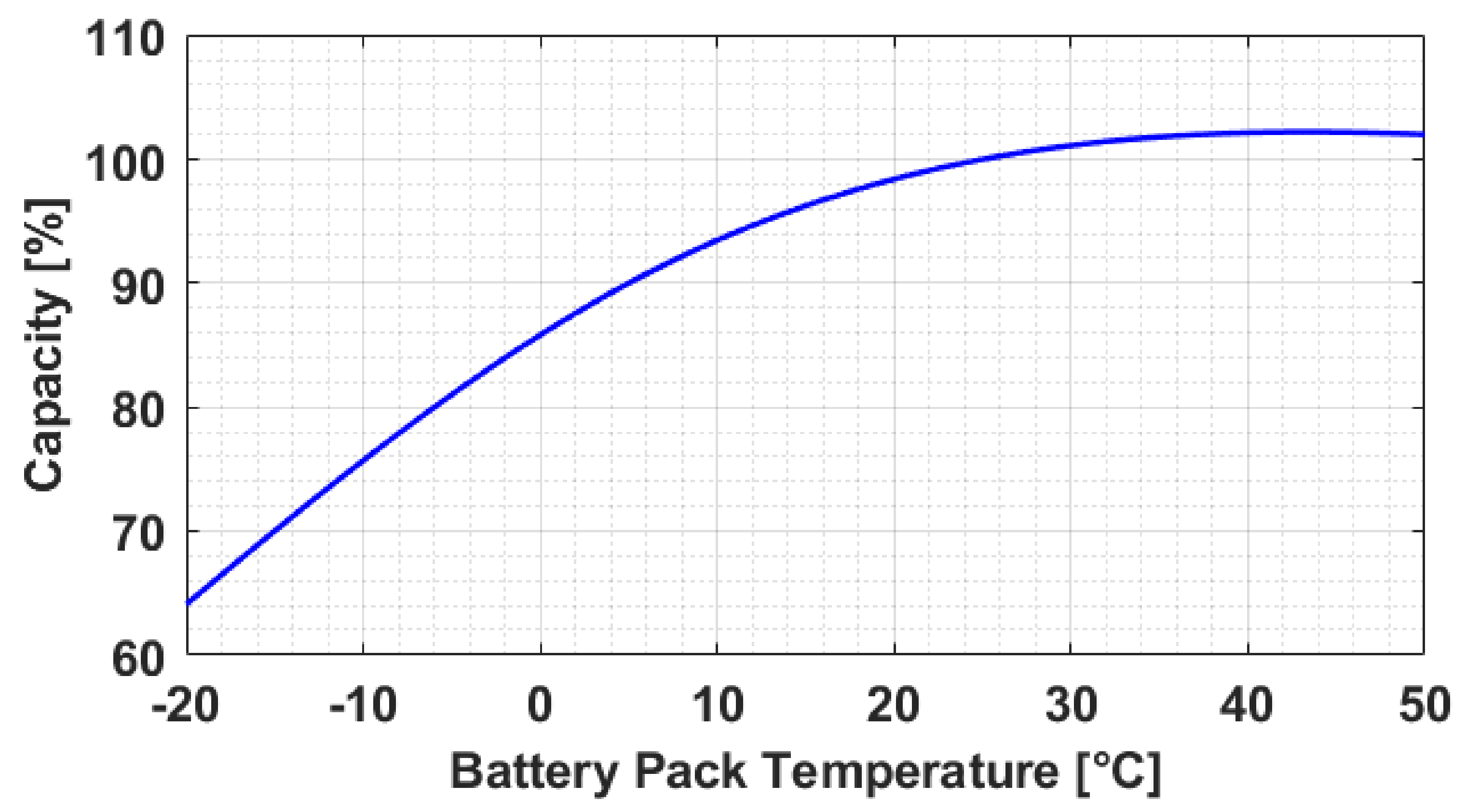
In terms of the correction factor for the battery pack temperature, the trend of the battery capacity as a function of the battery pack temperature is reported in Figure 7. A particular phenomenon was highlighted by temperatures over 25 °C as the battery capacity tended to overcome the nominal value. Nevertheless, high battery pack temperatures were typically responsible for producing faster aging and a drastic reduction in battery performance. More precisely, a reduction in the battery internal resistance and a higher frequency of over-discharging phenomena occurred, as shown in [26]. However, allowing the battery to work at any temperature level did not represent a beneficial solution.

The fluctuations of battery capacity due to a variation of the battery pack temperature was considered through the value ${\lambda }_{t_{bp}}$ in the range (0.64, 1.03).

With regard to the correction factor accounting for the reduction in battery capacity due to its SoH, the trend shown in Figure 8 was considered for the analyses. To clarify, a life-cycle was considered as a complete discharge until the DoD was reached, followed by a complete recharge of the battery. It can be noted that a significant effect on the available capacity was produced by a change in the DoD. In fact, increasing the DoD can lead to an increase in the driving range of the vehicle but also to a reduction of the maximum life-cycles admitted. Specifically for the data shown in Figure 8, a DoD equal to 80% could allow the battery to improve the life cycles by 50%, increasing from 400 (with DoD equal to 100%) to 600 life-cycles. This value was selected on the assumption that it could represent the best trade-off between battery usage (i.e., battery longevity) and electric range.

Accordingly, two distinct scenarios were analysed in the present paper regarding ${\lambda }_{SoH}$: within the first scenario, the maximum DoD admitted was set to 100%; in the second scenario, the maximum DoD admitted was reduced to 80%. Within the two different scenarios, the reduction in battery capacity over time differs, as shown in Figure 9. According to the data extracted from [26,27], battery capacity showed a nearly flat trend in the case of DoD80 (blue curve), whereas a steeper reduction was observed for DoD100 (red curve), as the termination condition was found at 400 cycles. In the case of DoD100, a peak occurred in the early stages of battery life, and was related to over-discharging phenomena which were responsible for a very fast capacity fading (i.e., roughly −20% in 200 cycles). To clarify, the termination of both curves was correlated to the number of cycles at which 20% of the battery capacity was depleted.

Using the same approach as for ${\lambda }_{t_{bp}}$, the values of ${\lambda }_{SoH}$ were considered in the range (0.8, 1).

Once the available capacity of the battery was determined, a correct evaluation of the battery SoC was performed by producing a good estimation of the current flowing into the battery (see Equation (20)). To achieve this, the power required by the road (i.e., the traction/braking power) must be coupled with any further power demand. For a BEV, auxiliary loads assume a relevant role and therefore their inclusion in the model is needed [12]. Specifically, the larger amount of auxiliary power can be referred to cabin heating and cooling operations (i.e., HVAC). Within the present model, a reversible vapor compressor–heat pump (VC–HP) layout was considered as the vehicle’s HVAC system. This choice was made due to the higher reliability shown by the VC–HP relative to other systems (e.g., evaporative cooling integrated thermal management) [28], which has increasingly spread throughout the automotive market [29]. According to the R32 coolant [29] and based upon the model suggested in [30], the curve shown in Figure 10 was built considering HVAC power consumption $P_{HVAC}$ as a function of the ambient temperature, assuming the optimal cabin temperature is 24 °C ($T_{cabin}$). The model equations are:

$$P_{HVAC}=\left\{\begin{array}{ccc}0& & \mathrm{turned\; off}\\ P_{heat}\left(T_{cabin}-T_{air}\right)& \left[W\right]& \mathrm{heating\; mode}\\ P_{cool}\left(T_{air}-T_{cabin}\right)& & \mathrm{cooling\; mode}\end{array}\right.$$

(23)

As highlighted in Figure 10, power consumption has always been considered as a positive value. A baseline of 50 W was used to account for the fans’ load. Moreover, human metabolic heat was taken into account, given the relatively small volume of an L-7 quadricycle cabin. The formulation of the metabolic power is:

$$Q_{met}=\dot{met}\ast BSA=\left\{\begin{array}{cc}147 \left[W\right]& \mathrm{driver}\\ 95 \left[W\right]& \mathrm{passenger}\end{array}\right.$$

(24)

in which $Q_{met}$ is the metabolic power, $\dot{met}$ is the metabolic rate and $BSA$ is the body surface area. To clarify, a fixed BSA based on the European average value (1.73 m²) [31] was considered whereas two different metabolic rates accounted for the driver and the passenger (85 W/m² for the driver and 55 W/m² for each passenger) [32]. The heat produced by human bodies was added when the system was under cooling conditions, whereas it was subtracted under heating mode. No other thermal loads were considered in the study (e.g., sun irradiation) since they represent a minor impact on overall HVAC consumption [30]. As a final contribution, the sum of the loads coming from any other vehicle auxiliary (e.g., headlights, electric wipers, electric power window, etc.) was fixed at 200 W.

Once $\int I_{batt} dt$ had been calculated, the Equivalent Battery Voltage (EBV) [25] can be defined according to the following equation:

$$EBV\left(t\right)=\frac{{{\displaystyle \int }}_{t_0}^{t^{\ast }}v\left(t\right)i\left(t\right)dt}{{{\displaystyle \int }}_{t_0}^{t^{\ast }}i\left(t\right)dt} \left[V\right]$$

(25)

where $v\left(t\right)=OC{V}_{batt}$, $i\left(t\right)=I_b$ while $t_0$ and $t^{\ast }$ are the initial and final time steps of the driving mission, respectively. According to (25), the EBV refers to the entire driving mission. The energy consumption of the vehicle $EC$ over the mission can be calculated as follows:

$$EC=\frac{EBV\ast \int I_b dt}{1000} \left[kWh\right]$$

(26)

According to [25], the electric vehicle energy index is computed as:

$$ei=\frac{d}{EC} \left[\raisebox{1ex}{$km$}\!\left/ \!\raisebox{-1ex}{$kWh$}\right.\right]$$

(27)

in which $d$ represents the number of kilometers that could be travelled by the vehicle with an energy consumption of 1 kWh. Finally, the BEV residual range can be estimated as:

$$rr=\left(C_{disp}-EC\right)\ast ei \left[km\right]$$

(28)

in which $C_{disp}$ is the battery available capacity estimated through:

$$C_{disp}=So{C}_i\ast {\lambda }_{t_{bp}}\ast {\lambda }_{SoH}\ast C_b \left[kWh\right]$$

(29)

where $So{C}_i$ is the initial value of the battery SoC for a given driving mission. According to this procedure, a more precise evaluation of both $I_b$ (including the power demanded by the auxiliaries) and $C_{disp}$ (considering thermal conditions and battery ageing) can be performed and, hence, a more reliable estimation of the real residual driving range can be obtained.

3. Results

In this section, the results of the analyses are presented according to the set of simulations carried out for the L7e vehicle considered in the STEVE project [23] and based on a dataset made of thirty driving missions recorded during an experimental testing campaign held in Turin (IT). For simplicity, only a sub-set of four different velocity profiles were employed for assessing the performance of the vehicle model. The real driving missions are reported in Figure 11 while their relative battery SoC trajectories are shown in Figure 12. An acronym “DMXX” will be used for identifying the driving missions, with “XX” standing for the acquisition number of the driving mission during the testing campaign. As can be seen in Figure 11, different distances were covered during the experimental driving tests, and a maximum velocity was achieved at roughly 50 km/h. The shape of the velocity trajectory differed from one test to the other as the road, traffic and driver behaviour could change. In terms of battery SoC trajectories, multiple SoC starting points were included in the study. The validation of the model presented in Section 2.2 has been performed based on the experimental battery SoC profiles and employing the vehicle velocity trajectories as inputs of the backward-facing approach. Such an operation was the achievement of a fundamental milestone, before stepping into the application of the model presented in Section 2.3.

To give a more comprehensive view of the whole experimental dataset, some of the main characteristics of each acquired driving mission were statistically processed and are reported through the charts of Figure 13, where the histograms show the distribution of travelled distance, mean velocity, maximum acceleration and maximum SoC variation achieved throughout the driving missions.

The vehicle specifications and model parameters considered in the analyses are reported in

Table 2. Vehicle technical specifications.

General Specifications
Vehicle homologation class	L7
Kerb weight [kg]	650
Vehicle front/rear weight distribution [%]	54/46
Vehicle dimensions
Wheelbase [mm]	1815
Width [mm]	1500
Height [mm]	1565
Minimum ground clearance [mm]	165
Motor-generator
Peak power [kW]	12
Rated power [kW]	6.3
Battery
Battery voltage [V]	72
Battery capacity [Ah]	140

and

Table 3. Model parameters.

Vehicle mass [kg]	898
Coefficient of rolling resistance	0.006
Wheels rolling radius [m]	0.257
Vehicle frontal area [m2]	2.14
Drag coefficient	0.65
Final drive speed ratio	3.6
Final drive efficiency	0.97
Gearbox transmission ratio	[2–4.5]
Gearbox efficiency	[0.97–0.98]
Auxiliary power request [W]	200
AC/DC converter efficiency	0.95
Saturation current [A]	50

, respectively. With regard to the model parameters, a small sub-set of data (Table 3, highlighted rows) had to be assumed from the literature because of an uncertainty in the original data.

A preliminary validation of the model was performed by comparing the experimental and estimated battery discharges along the different driving missions. To this end, the evaluation of the residual driving range has not been included in this first analysis. The results obtained by the application of the model on the experimental missions DM09, DM15, DM20 and DM25 are reported in

Table 4. Results of the model validation on DM09, DM15, DM20 and DM25 based on the final values of the battery state of charge.

Driving Mission	$\mathit{S}\mathit{o}{\mathit{C}}_{\mathit{T}}^{\mathit{e}\mathit{x}\mathit{p}}$	$\mathit{S}\mathit{o}{\mathit{C}}_{\mathit{T}}^{\mathit{s}\mathit{i}\mathit{m}}$	Relative Difference
DM09	0.910	0.899	1.10%
DM15	0.850	0.847	0.23%
DM20	0.920	0.921	−0.14%
DM25	0.700	0.703	−0.30%

considering the model parameters of Table 3. In the table, for each DM the experimental ($So{C}_T^{exp}$) and estimated ($So{C}_T^{sim}$) battery SoC final values are reported in the second and third columns, respectively, together with their relative difference in percentage (last column). The BEV model showed a promising accuracy in terms of battery SoC estimation and a good adaptability when tested under very different driving conditions. In fact, the maximum relative difference peaked at 1.1% for DM09, whereas smaller values were obtained for the other experimental missions. Nevertheless, an additional validation of the model was conducted in order to thoroughly assess for any possible leak in the non-experimental model parameters of Table 3. A tuning operation of these parameters was performed through several sensitivity analyses, which involved the vehicle mass, the saturation current at the AC/DC converter level and the drag coefficient. Finally, the implementation of the model for the estimation of the BEV residual driving range was performed taking into account battery aging, HVAC consumptions and BTMS power demands (i.e., battery preheating).

3.1. Model Validation

In this section, the results of the tuning operation over the vehicle mass, the saturation current at the AC/DC converter level and the drag coefficient are presented. Specifically, the effects of the mono-dimensional variation of each model parameter on the battery SoC trajectory estimated by the model are reported.

3.1.1. Vehicle Mass

The vehicle mass is considered as the sum of four different factors:

$$m_{veh}=m_{body}+m_{driver}+m_{pass}+m_{payload}$$

(30)

where $m_{body}$ is the kerb mass,$m_{driver}$ is the weight of the driver, $m_{pass}$ is the weight of the passenger and $m_{payload}$ is the mass of an additional mass in the vehicle. Five different scenarios were assumed for the analysis as reported in

Table 5. Vehicle masses considered in the tuning operation.

Scenario		Vehicle Mass
1	Driver only	720 kg
2	Driver w/light payload (30 kg)	750 kg
3	Driver and Passenger	790 kg
4	Driver, Passenger w/light payload	820 kg
5	Gross vehicle mass	898 kg

. In the second and third columns, the details of the scenario and the relative considered vehicle mass have been reported, respectively.

The battery SoC trajectories resulting from the application of the BEV model on DM15 are charted in Figure 14 and compared with the experimental trajectories. To clarify, the decreasing step trend of the battery SoC curve (green) was due to the precision of the sensors mounted on the vehicle during the experimental testing campaign. Specifically for DM15, the change in vehicle mass was responsible for a variation of the final battery SoC value between 0.928 and 0.920. The maximum relative difference between the final SoC values was therefore about 1%. The same analysis was performed on each driving mission sourced from the STEVE project testing campaign. For simplicity, the charts are not reported since the same trend was highlighted in the entire dataset and the variation of the final battery SoC value was in the range (0.3, 1)%. According to this result, the mass variation given by scenarios in Table 5 has not been considered as a highly influencing factor of the charge consumed and hence the battery SoC evolution through time. However, the gross vehicle mass was assumed for all following analyses since it better fitted the different driving missions considered in the study (see Figure 14).

3.1.2. Saturation Current

A second analysis was performed regarding the maximum current admitted during regenerative braking conditions (i.e., saturation current) at the AC/DC converter level. Recalling Section 2.2, a fixed AC/DC converter efficiency was assumed, whereas four different values of the saturation current $I_{sat}$ admitted in the system were considered. The details of the tested scenarios are reported in

Table 6. Saturation currents considered in the tuning operation.

Scenario	Saturation Current
1	25 A
2	50 A
3	75 A
4	experimental

. In the first three scenarios, typical saturation current values were imposed on the BEV model despite the driving mission profile. In the fourth (Table 6, last row), the value of $I_{sat}$ was set to the indirectly estimated value using the experimental battery SoC trajectories of the different driving missions. As an example, the actual values of the recharging current obtained throughout DM25 are reported in Figure 15.

The blue curve is representative of the actual values of the current flowing into the battery during any regenerative braking event, whereas the dashed red curve is representative of the vehicle velocity profile. The recharging current assumed a positive value only in a sub-set of the entire driving mission time steps, since it was activated only when braking scenarios occurred. Specifically for DM25, the maximum recharging current seen by the system was roughly 120 A. Recalling the saturation currents considered in Table 6, the experimental saturation current for DM25 in the last scenario (#4) was set to 120 A.

The comparison between the experimental battery SoC profile and those produced by the model when applied to DM25 in case of the four different recharging currents is reported in Figure 16.

Of note, the difference between the battery SoC curves throughout the mission is quite negligible. Two reasons may account for this result: first, the share of breaking events (and their related time) with respect to the entire driving duration is relatively small (~8%); second, the variation of the charge consumed calculated by the integral of (22) according to the ECC method is mostly mitigated and its effects are reduced. In the case of DM25, the final battery SoC value fluctuated in the range (0.705, 0.695) (~1% of maximum relative variation). Since the final battery SoC variation can be considered as irrelevant and that the same results occur for the entire dataset, the experimental $I_{sat}$ values have hence been considered for any further analysis.

3.1.3. Drag Coefficient

Among the vehicles classified as L-7, very different shapes can be seen on the global market, which are characterised by distinct drag coefficients. Since L-7 vehicles are typically adopted under urban driving conditions, moderate velocities and accelerations are exploited. Therefore, the aerodynamics shared due to the chassis geometry might produce a minor contribution to the variation of the battery SoC trajectory.

Nevertheless, very different scenarios have been selected to assess for the real effects of the drag coefficient on the real driving missions considered in this study. In fact, the drag coefficient changed, starting from a very low value of 0.35 to an extremely high 0.80, with a step of 0.05. The results produced by the model when applied to DM25 are reported in Figure 17.

It is noted that the shapes of the battery SoC and their relative final values are very distinct. In fact, the estimated trajectories start diverging after 500 s with a maximum variation of the final value fluctuating roughly between 0.665 and 0.60 (i.e., 6.5%). The latter is larger than the one occurring when the vehicle mass and saturation current are changed. As a result, it is important to consider that a very large range of variation of the drag coefficient was considered in the present analysis. In fact, drag coefficients down to 0.35/0.4 are typically related to sport cars [33] whereas values higher than 0.7 are typically representative of lorries or American automobiles designed between the 1920s and 1930s [34]. Repeating the tuning operation on the entire set of driving missions, the maximum variations of the final battery SoC fluctuation were calculated between 0.5% and 6.5%, with a higher influence noticed in the driving missions featured by higher velocities. Finally, since the majority of experimental battery SoC trajectories were validated by applying a drag coefficient equal to 0.65 (see Figure 17), the latter has been set for all further analysis.

3.2. Combined Effect of Battery Aging and Battery Pack Temperature Variation on the Residual Driving Range of a BEV

An investigation about the realistic performance of the BEV considered in the study was performed by introducing the correction factors of (22) in the calculation of the available battery capacity.

As a first step, a failure of BTMS was assumed in order to analyse the possible impact of the battery pack temperature on battery capacity fading, and the combined effect with different battery ageing levels was analyzed. Concerning ${\lambda }_{SoH}$, two different conditions were considered as the DoD was set at 100% and at 80% (see Section 2.3). On the other hand, three different scenarios were studied for the battery pack temperature (hence ${\lambda }_{t_{bp}}$) as reported in

Table 7. Temperatures of the battery pack.

Scenario	Reference Temperature	Temperature Range
1	0 °C	(−2.5, 2.5) °C
2	15 °C	(12.5, 17.5) °C
3	22.5 °C	(20, 25) °C

. Each scenario included a reference temperature and a +/−2.5 °C variation range. The temperature evolution throughout the driving mission was estimated by means of a piecewise cubic Hermite interpolating polynomial [35] method. According to the latter, the shape of battery pack temperature varied around the central reference value and within the imposed variation range.

The results were divided in the two following sections based on the DoD assumed during the analyses, specifically a complete discharge with DoD100 and a partial discharge with DoD80.

3.2.1. Complete Discharge (DoD100)

In this section, the results obtained by considering a variation of the battery pack temperature in the range (−2.5, 2.5) °C are reported for DM25. To this end, four different battery ageing levels were assumed: 0, 200, 300, 400 life-cycles completed. The combined effects of the variation of the battery pack temperature with the four different battery ageing levels are reported in Figure 18, Figure 19, Figure 20 and Figure 21. The red curve represents the variation of the battery pack temperature, the blue curve represents ${\lambda }_{tot}$, the green curve represents ${\lambda }_{t_{bp}}$ and the black line represents ${\lambda }_{SoH}$ in the case of DoD100 (${\lambda }_{So{H}_{DoD100}}$). The latter is a line (and not a curve) since it assumed a constant value over the mission for a given battery ageing level, whereas it can be reduced when the number of life-cycles completed by the battery is increased. In Figure 18, the battery is considered as new (0 life-cycles completed) and hence ${\lambda }_{So{H}_{DoD100}}=1$; in Figure 19, the battery completed 200 life-cycles (i.e., ${\lambda }_{So{H}_{DoD100}}=0.985$); in Figure 20, the battery completed 300 life-cycles (i.e., ${\lambda }_{So{H}_{DoD100}}=0.88$) while in Figure 21 the battery reached 400 life-cycles (i.e., ${\lambda }_{So{H}_{DoD100}}=0.8$), which represents the battery EoL (see Figure 9).

As far as the number of life-cycles was increased (i.e., the value of ${\lambda }_{So{H}_{DoD100}}$ was reduced), the curve of ${\lambda }_{tot}$ was relevantly downshifted (average values from ~0.85 with new battery pack down to ~0.68 with an old battery). On the other hand, considering a quasi-random variation of the battery pack temperature within a 5% variation range did not introduce a significant effect on the global correction factor.

3.2.2. Partial Discharge (DoD80)

The combined effect of the variation of the battery pack temperature and the battery ageing level is presented in this section for DM 25 in the case of DoD80. Recalling Figure 9, four different values of the life-cycles completed by the battery were considered, specifically 0, 200, 400 and 600 (EoL). The charts from Figure 22, Figure 23, Figure 24 and Figure 25 report the results obtained for 0 (i.e., ${\lambda }_{So{H}_{DoD80}}=1$), 200 (i.e., ${\lambda }_{So{H}_{DoD80}}=0.985$), 400 (i.e., ${\lambda }_{So{H}_{DoD80}}=0.94$) and 600 life-cycles (i.e., ${\lambda }_{So{H}_{DoD80}}=0.8$), respectively.

The general trend shown by the results of Section 3.2.1 recurred in the case of a partial discharge with DoD80. In fact, the average value of ${\lambda }_{tot}$ started decreasing at around 1/3 of the battery EoL (~0.85) and kept decreasing until the EoL was achieved (~0.67). Once again, the influence of the variation of ${\lambda }_{t_{bp}}$ did not show relevant effects on the global correction factor.

The battery SoH had much greater impact than a relatively contained variation of the battery pack temperature on ${\lambda }_{tot}$ and hence on the available battery capacity, in both DoD100 and DoD80 scenarios. This result could also be expected in the cases of Scenarios 2 and 3 of Table 7, because the average value of ${\lambda }_{t_{bp}}$ would be higher with respect to Scenario 1 since the battery pack temperature would be closer to the optimal operating temperature. Therefore, Scenario 1 can be considered as the most demanding from a battery temperature perspective, and hence, no results related to Scenario 2 and 3 are reported for conciseness.

As a final step, the effects of the decay of ${\lambda }_{tot}$ were further investigated by analysing the evolution of the battery SoC and the residual driving range estimated along the driving missions. These results are reported in the next section.

3.2.3. Residual Range

Since the correction factor ${\lambda }_{tot}$ plays a crucial role in the definition of the battery available capacity and hence on the variation law of the battery SoC during a driving mission, the reduction in ${\lambda }_{tot}$, evaluated with different battery pack temperature and ageing levels, was used to estimate the variation of the residual range of the BEV exploited in this paper.

In Figure 26 and Figure 27, the curves of battery SoC and residual driving range are charted, respectively, accounting for the four different battery ageing levels considered in Section 3.2.1 (DoD100). As far as the battery EoL was achieved (purple curve), the tendency of the battery SoC evolution grew progressively resulting in lower final battery SoC values. Consistently, an important reduction in the BEV residual driving range occurred with a relevant loss of both the first (from ~60 km down to ~46 km) and last residual range estimations (from ~48 km down to ~37 km) made at the beginning and at the end of the driving mission, respectively.

The same analysis was conducted for DoD100. The effect of the decay of ${\lambda }_{tot}$ on battery SoC and residual driving range are reported in Figure 28 and Figure 29, respectively. In this case, a smaller variation of both battery SoC and BEV residual driving range occurred until 2/3 of the entire life-span of the battery (400 life-cycles). Conversely, once the battery EoL was reached, the loss in the residual range became much more relevant.

In conclusion, despite the absolute number of kilometers that could be driven permitting a complete discharge of the battery, the DoD80 appears to be a more efficient condition for battery operation since it allows for mitigation of the negative effects related to the reduction in the correction factor of the battery available capacity.

3.3. Effect of HVAC Power Demand on the Residual Range of a BEV

The influence of HVAC power demands over the battery SoC evolution and the residual driving range estimated throughout the driving mission were studied and the results are reported here. Both conditions of heating and cooling the vehicle cabin were simulated considering ambient temperatures (outside the vehicle) equal to 0 °C (winter scenario) and 35 °C (summer scenario), respectively. The HVAC system was assumed to be switched on only 60 s after the beginning of the drive and the relative power demand was calculated according to (23) and Figure 10. A comparison of battery SoC and residual range variation along DM20 with and without HVAC consumption for the winter scenario are reported in Figure 30 and Figure 31, respectively. The evolution of the battery SoC charted in Figure 30 highlights two different trends, with final SoC values differing by about 4%. Consistently, the trajectories of the residual driving range estimated throughout DM20 followed very different traces. Specifically, the curve of the residual driving range estimated when the HVAC was activated (Figure 31, blue curve) shows a relevant decrease after 60 s, which is the time instant at which the HVAC was assumed to be turned on. At this stage, the power consumption demanded for the air conditioning was instantly added to the battery, and hence a drastic fall occurred to the curve. From that time instant onwards, the estimated residual driving range stabilised to a similar decreasing shape of the HVAC-off curve and led to a final variation of −31% (−35 km).

The same analysis was conducted considering the summer scenario with an ambient temperature of 35 °C and the results for DM20 are reported in Figure 32 and Figure 33. Once again, the influence of the cabin conditioning system assumed a relevant role both on the battery SoC discharge and the residual driving range, which were reduced by 7% and 46% (−51 km) with respect to the HVAC-off condition, respectively.

Considering the entire dataset under HVAC-on condition, the final values of the battery SoC reduced in the range (4, 12)% for heating mode and (3, 15)% for cooling mode, whereas the average decrease in residual driving range stayed between (28, 57)% for heating mode and from (25, 63)% for cooling mode. The HVAC consumption for cabin conditioning can hence be considered as a major impact for BEV real-world driving missions in both cases of hot and cold ambient temperatures.

3.4. Effect of Battery Pre-Heating on the Residual Driving Range of a BEV

Since the battery pack temperature directly influences the available battery capacity through the correction factor ${\lambda }_{t_{bp}}$, a typical thermal management is performed by the BTMS to control the temperature fluctuations over time, bounding them within proper temperature limits. Therefore, the influence of the additional power consumption required by the BTMS over the residual driving range of a BEV was assessed and the results of the analysis are reported in this section. In terms of the BTMS consumption, the effective power demand depends upon the type of thermal management performed.

In the present paper, self-heating and air-cooling thermal managements were considered for the modeled L-7 BEV in the case of cold and hot battery conditions, respectively. Basically, self-heating the battery translated into an additional consumption of an amount of battery energy to heat the battery up to a certain range. On the other hand, placing the battery pack in a location with a large air flux permitted its passive cooling. To this end, [36] demonstrated that an active cooling approach would not lead to relevant improvements with respect to passive cooling for small vehicle applications. Therefore, considering an optimal battery pack temperature in the range of 15 and 30 °C, thermal management was modelled considering a self-heating approach which aimed at pushing the temperature into the optimal range, and a passive cooling approach which neglects the temperature to exceed the upper threshold by cutting the MG power output. To clarify, the optimal range of battery temperature was selected according to VRLA batteries, for which high temperatures could result in battery dry out [37] and an optimal operating temperature was identified at 20 °C. The heating specific energy consumption related to self-heating was calculated based on the temperature difference between the actual battery pack temperature and 20 °C by means of a linear characteristic which starts in the origin and reaches 8.5 Wh/kg at temperature differences of 30 °C [38]. The effect of the BTMS consumption on the battery SoC and residual driving range evolution throughout DM09 was assessed by considering a pre-heating action on the vehicle. The latter consisted of self-heating the battery while the vehicle was in a stationary location (stopped) and the system was turned on. Due to the pre-heating action, the driver could enter the vehicle and start driving with the battery ready to operate in the optimal temperature region. Even though battery pre-heating added a power consumption to the system in the early stages of a driving mission, beneficial effects on ${\lambda }_{t_{bp}}$ could be realized with respect to non-thermal management conditions as the optimal temperature range was achieved.

In Figure 34 and Figure 35, the estimated residual driving range curves are charted considering an initial battery pack temperature of 0 °C and −10 °C, respectively. The BTMS-off case (red curve) considers a ${\lambda }_{t_{bp}}$ range of variation between (0.745, 0.766) and (0.849, 0.867) for an initial battery temperature of 0 °C, and −10 °C, respectively. It is noted that the initial estimation of the residual driving range appeared to be worse for the BTMS-on condition (blue curve) compared to the BTMS-off condition. This is due to the initial estimation of the battery capacity loss which is directly linked to the amount of energy that has to be devoted to heat the battery temperature up to the optimal operating temperature. Specifically, for an initial temperature of 0 °C, the gap of temperature was 23 °C whereas an increase of 33 °C was needed for an initial temperature of −10 °C. The time step at which the vehicle velocity profiles assumed the first positive value differed for the BTSM-on and BTMS-off conditions since BTMS-on assumes the vehicle remains in the same location (e.g., parking lot) while heating up the battery. Once the battery heating up process has completed, the vehicle was assumed to run the same driving mission and hence a shift ahead of the blue curves with respect to the red curves appears in the charts. The main result highlighted by Figure 34 and Figure 35 is that, due to the increase in the value of ${\lambda }_{t_{bp}}$ in terms of battery pre-heating, and considering a fixed value of ${\lambda }_{SoH}$ (i.e., fixed amount of life-cycles completed by the battery), the available capacity grows through time allowing for higher residual driving ranges. To clarify, the value of ${\lambda }_{t_{bp}}$ could be increased to (0.95, 1) for pre-heating mode due to BTMS thermal management. A non-utilisation of the thermal management therefore led to a considerable loss of BEV electric range when the vehicle was turned on in a very cold driving environment. Moreover, the higher the difference between the initial operating temperature of the battery and its optimal operating temperature, the greater the amelioration that can be applied to the system through a proper exploitation of the BTMS control. Indeed, such an effect could naturally be mitigated only when warmer ambient temperatures are encountered, as a lower difference between the operating battery temperature and its optimal operating temperature would be experienced (i.e., ${\lambda }_{t_{bp}}$ tends to 1).

Thanks to this set of analyses, the positive influence of pre-heating the battery pack when the vehicle is parked in a cold environment has been demonstrated.

4. Discussion

In the present study, a model for a realistic estimation of the residual driving range of a BEV has been developed including the effects of battery pack temperature and battery ageing level, HVAC consumption and battery pre-heating. Accordingly, an L-7 BEV has been modelled through a backward-facing approach and validated by means of real-world data acquired during the STEVE project [23]. Since the experimental driving missions included real driving data, this meant that driver behaviour, road and traffic conditions could also be exploited in the analyses. Therefore, the results presented in this paper can be considered as representative of the combined effect of the above-mentioned factors on the real driving range of a BEV and follow-up research based on [12]. An ECC method was chosen to perform the estimation of the battery SoC to be used for calculating the vehicle residual driving range. In this paper, differently from Zhao et al. [39], the validation of the experimental battery SoC profiles related to real-world driving missions allowed for optimizing the usage of the ECC method, since real information about the initial battery SoC could be exploited, and no approximations were required to be introduced in the analyses.

Once the validation of the BEV model on several experimental driving missions had been completed, the first set of analyses was aimed at assessing the battery ageing influence on the real residual driving range of the vehicle. To this end, two distinct DoD levels (80% and 100%) were considered. For each, four battery ageing levels (i.e., number of life-cycles completed) were evaluated and their influence on the battery available capacity was assessed. From a practical perspective, a variation of the correction factor ${\lambda }_{SoH}$ was made. Furthermore, the presence of a BTMS failure was assumed to include a variation of the second correction factor ${\lambda }_{t_{bp}}$ in the analysis. This condition was exploited to define the relative importance of each sub-correction factor on the global correction factor ${\lambda }_{tot}$. First, the predominance of the battery ageing level correction factor on the global correction factor (with respect to the battery pack temperature) was proved. Then, reducing the DoD from DoD100 to DoD80 demonstrated that a higher battery life-span and smaller variations of the battery available capacity could be achieved before achieving the battery EoL. In fact, roughly two thirds of the entire life-span of a battery could be operated with a negligible loss of the battery available capacity, in the case of DoD80, whereas only one third could be operated in the same condition when DoD100 was considered. It is worth highlighting that range anxiety and safety buffer are directly linked to trip mileage [40], therefore, experiencing a fast decay of the battery performance (i.e., available capacity) might lead to a deterrent effect for new BEV drivers. Of note, the selection of a higher DoD (e.g., DoD100) would lead to temporarily larger driving ranges which would be lost in the long term.

Another important analysis focused on the effect of HVAC consumption on the entire system, both for heating and cooling the vehicle cabin (i.e., cold and hot ambient temperatures). HVAC consumption was modelled assuming an optimal cabin temperature of 24 °C, and that the HVAC power demand would increase when the cabin temperature moved below or above the optimal temperature. Additional auxiliary power was included in the study, but HVAC was assumed to claim the main auxiliary power demand, according to [22]. As expected for a BEV, the battery SoC evolution and the residual driving range estimations proved to be largely affected when the HVAC system was turned on. A relevant loss was observed both for the battery SoC value and the residual driving range at the end of the driving missions. For this reason, an immediate solution could be to not activate the air conditioning system [41] when driving in urban environments and/or for short trips; on the other hand, BEV performance losses must be accepted for cold and hot ambient temperatures due to the activation of the entire HVAC system.

Finally, an assessment of the effects produced by pre-heating the battery before driving the vehicle was carried out when considering the vehicle parked in a cold environment (i.e., 0 °C and −10 °C). The results emphasised that battery pack pre-heating can be an interesting solution to ensure good vehicle performances (i.e., reducing the decay of battery available capacity) even in very cold driving scenarios, while increasing the residual driving range. Considering the role of BTMS on the residual range is therefore to be considered as a crucial aspect in the reduction of driver range anxiety.

5. Conclusions

In the present paper, the results produced by a model for the estimation of the residual driving range of a L-7 BEV were reported. Several factors were included in the analyses, such as battery ageing, battery pack temperature, HVAC consumption and pre-heating through BTMS-related thermal management, to provide the reader with a comprehensive view of a larger set of parameters to be included when a realistic definition of the driving range of BEV is achieved. The data used for testing the model for the estimation of the residual driving range were extracted from an experimental campaign held within the H2020 STEVE project.

First, the L-7 BEV backward-facing kinematic model was developed and validated on the experimental data. Then, the combined effect of battery ageing and battery pack temperature was assessed assuming a BTMS failure and four different amounts of battery ageing levels. The results proved the predominance of the ageing level on the overall performance of the battery and the convenience of shrinking the depth of discharge band in order to contain the loss of battery available capacity over time. After that, the effect of the HVAC power demand for heating and cooling the vehicle cabin on the BEV residual driving range was evaluated for winter and summer conditions, respectively. The results proved that an extended usage of the cabin conditioning system could be relevantly disadvantageous, even for a small BEV, regarding the reduction in vehicle performance. Finally, the convenience of pre-heating the battery through proper thermal management of the BTMS was assessed assuming the vehicle to be initially parked at 0° and −10 °C. Thanks to this analysis, the possibility of containing the reduction in the residual driving range by means of a pre-heating approach has been demonstrated. Furthermore, the amelioration given by employing the BTMS thermal management has been proved as much more efficient when the difference between the environment temperature and the optimal battery operating temperature increases.

Our next research will focus on the development and validation of a battery ageing prediction model to replace the look-up table approach. In addition, an analysis of the benefits brought by a proper control policy of the HVAC on the performance of a BEV will be carried out. Finally, a smart thermal management policy of the BTMS will be studied to optimize the battery heating and cooling processes for different driving conditions.

References

1. Allen, S.K.; Barros, V.; Burton, I.; Campbell-Lendrum, D.; Cardona, O.D.; Cutter, S.L.; Dube, O.P.; Ebi, K.L.; Field, C.B.; Handmer, J.W.; et al. Summary for Policymakers. In Managing the Risks of Extreme Events and Disasters to Advance Climate Change Adaptation; Cambridge University Press: Cambridge, UK, 2012; Volume 9781107025, ISBN 9781139177245. [Google Scholar]
2. Emissions of Air Pollutants from Transport—European Environment Agency. Available online: https://www.eea.europa.eu/data-and-maps/indicators/transport-emissions-of-air-pollutants-8/transport-emissions-of-air-pollutants-8 (accessed on 30 August 2021).
3. Transport: Increasing Oil Consumption and Greenhouse Gas Emissions Hamper EU Progress towards Environment and Climate Objectives—European Environment Agency. Available online: https://www.eea.europa.eu/publications/transport-increasing-oil-consumption-and/increasing-oil-consumption-and-ghg (accessed on 30 August 2021).
4. Osei, L.K.; Ghaffarpasand, O.; Pope, F.D. Real-World Contribution of Electrification and Replacement Scenarios to the Fleet Emissions in West Midland Boroughs, UK. Atmos 2021, 12, 332. [Google Scholar] [CrossRef]
5. Pevec, D.; Babic, J.; Carvalho, A.; Ghiassi-Farrokhfal, Y.; Ketter, W.; Podobnik, V. Electric vehicle range anxiety: An obstacle for the personal transportation (r)evolution? In Proceedings of the 2019 4th International Conference on Smart and Sustainable Technologies (SpliTech), Split, Croatia, 18–21 June 2019. [Google Scholar] [CrossRef]
6. Neubauer, J.; Wood, E. The impact of range anxiety and home, workplace, and public charging infrastructure on simulated battery electric vehicle lifetime utility. J. Power Sources 2014, 257, 12–20. [Google Scholar] [CrossRef]
7. Tannahill, V.R.; Sutanto, D.; Muttaqi, K.M.; Masrur, M.A. Future vision for reduction of range anxiety by using an improved state of charge estimation algorithm for electric vehicle batteries implemented with low-cost microcontrollers. IET Electr. Syst. Transp. 2015, 5, 24–32. [Google Scholar] [CrossRef]
8. Bonges, H.A.; Lusk, A.C. Addressing electric vehicle (EV) sales and range anxiety through parking layout, policy and regulation. Transp. Res. Part A Policy Pract. 2016, 83, 63–73. [Google Scholar] [CrossRef] [Green Version]
9. Rauh, N.; Franke, T.; Krems, J.F. Understanding the impact of electric vehicle driving experience on range anxiety. Hum. Factors 2015, 57, 177–187. [Google Scholar] [CrossRef] [PubMed]
10. Pevec, D.; Babic, J.; Carvalho, A.; Ghiassi-Farrokhfal, Y.; Ketter, W.; Podobnik, V. A survey-based assessment of how existing and potential electric vehicle owners perceive range anxiety. J. Clean. Prod. 2020, 276, 122779. [Google Scholar] [CrossRef]
11. Faraj, M.; Basir, O. Range anxiety reduction in battery-powered vehicles. In Proceedings of the 2016 IEEE Transp. Electrif. Conf. Expo, ITEC 2016, Dearborn, MI, USA, 27–29 June 2016. [Google Scholar] [CrossRef]
12. Varga, B.O.; Sagoian, A.; Mariasiu, F. Prediction of Electric Vehicle Range: A Comprehensive Review of Current Issues and Challenges. Energies 2019, 12, 946. [Google Scholar] [CrossRef] [Green Version]
13. Ng, K.S.; Moo, C.S.; Chen, Y.P.; Hsieh, Y.C. Enhanced coulomb counting method for estimating state-of-charge and state-of-health of lithium-ion batteries. Appl. Energy 2009, 86, 1506–1511. [Google Scholar] [CrossRef]
14. Ramoni, M.O.; Zhang, H.-C. End-of-life (EOL) issues and options for electric vehicle batteries. Clean Technol. Environ. Policy 2013 156 2013, 15, 881–891. [Google Scholar] [CrossRef]
15. Raman, N.; Chagnon, G.; Nechev, K.; Romero, A.; Sack, T.; Saft, M. Saft high power Li-Ion automotive battery technology. In Proceedings of the 20th International Electric Vehicle Symposium and Exposition, Long Beach, CA, USA, 15–19 November 2003; p. 12. [Google Scholar]
16. Qian, K.; Zhou, C.; Yuan, Y.; Allan, M. Temperature effect on electric vehicle battery cycle life in vehicle-to-grid applications. In Proceedings of the 2010 China International Conference on Electricity Distribution, CICED 2010, Nanjing, China, 13–16 September 2003. [Google Scholar]
17. Dubarry, M.; Liaw, B.Y.; Chen, M.S.; Chyan, S.S.; Han, K.C.; Sie, W.T.; Wu, S.H. Identifying battery aging mechanisms in large format Li ion cells. J. Power Sources 2011, 196, 3420–3425. [Google Scholar] [CrossRef]
18. Li, J.; Yuan, C.F.; Guo, Z.H.; Zhang, Z.A.; Lai, Y.Q.; Liu, J. Limiting factors for low-temperature performance of electrolytes in LiFePO4/Li and graphite/Li half cells. Electrochim. Acta 2012, 59, 69–74. [Google Scholar] [CrossRef]
19. Bloom, I.; Cole, B.W.; Sohn, J.J.; Jones, S.A.; Polzin, E.G.; Battaglia, V.S.; Henriksen, G.L.; Motloch, C.; Richardson, R.; Unkelhaeuser, T.; et al. An accelerated calendar and cycle life study of Li-ion cells. J. Power Sources 2001, 101, 238–247. [Google Scholar] [CrossRef]
20. Zhang, Z.; Li, W.; Zhang, C.; Chen, J. Climate control loads prediction of electric vehicles. Appl. Therm. Eng. 2017, 110, 1183–1188. [Google Scholar] [CrossRef]
21. Iora, P.; Tribioli, L. Effect of Ambient Temperature on Electric Vehicles’ Energy Consumption and Range: Model Definition and Sensitivity Analysis Based on Nissan Leaf Data. World Electr. Veh. J. 2019, 10, 2. [Google Scholar] [CrossRef] [Green Version]
22. El Khoury, G.; Clodic, D. Method of Test and Measurements of Fuel Consumption Due to Air Conditioning Operation on the New Prius II Hybrid Vehicle. SAE Tech. Pap. 2005, 114, 2563–2571. [Google Scholar] [CrossRef]
23. Smart-Taylored L-Category Electric Vehicle Demonstration in hEtherogeneous Urbanuse-Cases | STEVE Project | H2020 | CORDIS | European Commission. Available online: https://cordis.europa.eu/project/id/769944 (accessed on 30 August 2021).
24. Maino, C.; Misul, D.; Musa, A.; Spessa, E. Optimal mesh discretization of the dynamic programming for hybrid electric vehicles. Appl. Energy 2021, 292, 116920. [Google Scholar] [CrossRef]
25. Ceraolo, M.; Pede, G. Techniques for estimating the residual range of an electric vehicle. IEEE Trans. Veh. Technol. 2001, 50, 109–115. [Google Scholar] [CrossRef]
26. AGM vs Gel Batteries—Which Battery Type Is Better? Available online: https://www.canbat.com/guide-agm-batteries-gel-batteries/ (accessed on 30 August 2021).
27. 6-EVF-120 12V 120Ah(3hr) VRLA GEL BATTERY. Available online: http://en.chilwee.com:8000/upload/6-EVF-120.pdf (accessed on 30 August 2021).
28. Zhang, Z.; Wang, J.; Feng, X.; Chang, L.; Chen, Y.; Wang, X. The solutions to electric vehicle air conditioning systems: A review. Renew. Sustain. Energy Rev. 2018, 91, 443–463. [Google Scholar] [CrossRef]
29. Wu, J.; Zhou, G.; Wang, M. A comprehensive assessment of refrigerants for cabin heating and cooling on electric vehicles. Appl. Therm. Eng. 2020, 174, 115258. [Google Scholar] [CrossRef]
30. Sarrafan, K.; Sutanto, D.; Muttaqi, K.M.; Town, G. Accurate range estimation for an electric vehicle including changing environmental conditions and traction system efficiency. IET Electr. Syst. Transp. 2017, 7, 117–124. [Google Scholar] [CrossRef] [Green Version]
31. Sparreboom, A.; Verweij, J. Paclitaxel Pharmacokinetics, Threshold Models, and Dosing Strategies. J. Clin. Oncol. Off. J. Am. Soc. Clin. Oncol. 2016, 21, 2803–2804. [Google Scholar] [CrossRef]
32. ASHRAE Handbook—HVAC Applications—Building Operations and Management; SI Editions; ASHRAE: Atlanta, GA, USA, 2019; ISBN 9781936504077.
33. Dickison, M.; Ghaleeh, M.; Milady, S.; Subbakrishna, S.; Wen, L.T.; Al Qubeissi, M. Investigation into the aerodynamic performance of a concept sports car. J. Appl. Fluid Mech. 2020, 13, 583–601. [Google Scholar] [CrossRef]
34. Hucho, W.H.; Sovran, G. Aerodynamics of road vehicles. Annu. Rev. Fluid Mech. 1993, 25, 485–537. [Google Scholar] [CrossRef]
35. Piecewise Cubic Hermite Interpolating Polynomial (PCHIP)—MATLAB pchip. Available online: https://www.mathworks.com/help/matlab/ref/pchip.html (accessed on 31 August 2021).
36. Hémery, C.V.; Pra, F.; Robin, J.F.; Marty, P. Experimental performances of a battery thermal management system using a phase change material. J. Power Sources 2014, 270, 349–358. [Google Scholar] [CrossRef]
37. Ohmae, T.; Sawai, K.; Shiomi, M.; Osumi, S. Advanced technologies in VRLA batteries for automotive applications. J. Power Sources 2006, 154, 523–529. [Google Scholar] [CrossRef]
38. Pesaran, A.; Vlahinos, A.; Stuart, T. Cooling and preheating of batteries in hybrid electric vehicles. In Proceedings of the 6th ASME-JSME Thermal Engineering Joint Conference, Hawaii Island, HI, USA, 16–20 March 2003; pp. 1–7. [Google Scholar]
39. Zhao, L.; Lin, M.; Chen, Y. Least-squares based coulomb counting method and its application for state-of-charge (SOC) estimation in electric vehicles. Int. J. Energy Res. 2016, 40, 1389–1399. [Google Scholar] [CrossRef]
40. Yuan, Q.; Hao, W.; Su, H.; Bing, G.; Gui, X.; Safikhani, A. Investigation on Range Anxiety and Safety Buffer of Battery Electric Vehicle Drivers. J. Adv. Transp. 2018, 2018, 8301209. [Google Scholar] [CrossRef] [Green Version]
41. Huff, S.; West, B.; Thomas, J. Effects of Air Conditioner Use on Real-World Fuel Economy. SAE Tech. Pap. 2013, 2. [Google Scholar] [CrossRef]
Figure 1. Scheme of the BEV model with the main energy flows.
Applsci 11 09316 g001
Figure 2. High-resolution matrix for transmission ratio evaluation.
Applsci 11 09316 g002
Figure 3. Efficiency map of the reference motor-generator.
Applsci 11 09316 g003
Figure 4. Power and torque curves of the motor-generator.
Applsci 11 09316 g004
Figure 5. Battery cells open-circuit voltage as a function of the state of charge.
Applsci 11 09316 g005
Figure 6. Battery cells resistance as a function of the state of charge.
Applsci 11 09316 g006
Figure 7. Capacity variation as a function of the battery pack temperature.
Applsci 11 09316 g007
Figure 8. Trend of the battery life cycles as a function of the depth of discharge.
Applsci 11 09316 g008
Figure 9. Capacity fading in terms of battery depth of discharge equal to 80% (DoD80) and 100% (DoD100).
Applsci 11 09316 g009
Figure 10. HVAC consumption in cooling and heating modes.
Applsci 11 09316 g010
Figure 11. Velocity trajectories of the four experimental driving missions considered for the validation of the model.
Applsci 11 09316 g011
Figure 12. Battery state of charge trajectories of the four experimental driving missions considered for the validation of the model.
Applsci 11 09316 g012
Figure 13. Distribution of the travelled distance, mean velocity, maximum acceleration and battery state of charge variations for any driving mission in the entire experimental dataset.
Applsci 11 09316 g013
Figure 14. Comparison of the battery state of charge trajectories estimated by the model considering different vehicle masses with respect to the experimental battery state of charge of DM15.
Applsci 11 09316 g014
Figure 15. Recharging current during DM25.
Applsci 11 09316 g015
Figure 16. Comparison of the battery state of charge trajectories estimated by the model considering different saturation currents with respect to the experimental battery state of charge of DM25.
Applsci 11 09316 g016
Figure 17. Comparison of the battery state of charge trajectories estimated by the model considering different drag coefficients with respect to the experimental battery state of charge of DM25.
Applsci 11 09316 g017
Figure 18. Combined effect of the battery pack temperature and the battery ageing level on λ t o t for DM25 in the case of a new battery and DoD100.
Applsci 11 09316 g018
Figure 19. Combined effect of the battery pack temperature and the battery ageing level on λ t o t for DM25 in the case of a battery with 200 life-cycles completed and DoD100.
Applsci 11 09316 g019
Figure 20. Combined effect of the battery pack temperature and the battery ageing level on λ t o t for DM25 in the case of a battery with 300 life-cycles completed and DoD100.
Applsci 11 09316 g020
Figure 21. Combined effect of the battery pack temperature and the battery ageing level on λ t o t for DM25 in the case of a battery with 400 life-cycles completed and DoD100.
Applsci 11 09316 g021
Figure 22. Combined effect of the battery pack temperature and the battery ageing level on λ t o t for DM25 in the case of a new battery and DoD80.
Applsci 11 09316 g022
Figure 23. Combined effect of the battery pack temperature and the battery ageing level on λ t o t for DM25 in the case of a battery with 200 life-cycles completed and DoD80.
Applsci 11 09316 g023
Figure 24. Combined effect of the battery pack temperature and the battery ageing level on λ t o t for DM25 in the case of a battery with 400 life-cycles completed and DoD80.
Applsci 11 09316 g024
Figure 25. Combined effect of the battery pack temperature and the battery ageing level on λ t o t for DM25 in the case of a battery with 600 life-cycles completed and DoD80.
Applsci 11 09316 g025
Figure 26. Comparison of the battery SoC trend estimated for different battery ageing levels throughout DM25 in the case of DoD100.
Applsci 11 09316 g026
Figure 27. Comparison of the residual driving range estimated for different battery aging in the case of DoD100.
Applsci 11 09316 g027
Figure 28. Comparison of the battery SoC trend estimated for different battery ageing levels in the case of DoD80.
Applsci 11 09316 g028
Figure 29. Comparison of the residual driving range estimated for different battery aging in the case of DoD100.
Applsci 11 09316 g029
Figure 30. Evolution of the battery SoC variation with and without the HVAC system consumption for DM 20 considering the winter scenario (0 °C).
Applsci 11 09316 g030
Figure 31. Evolution of the residual range variation with and without the HVAC system consumption for DM 20 considering the winter scenario (0 °C).
Applsci 11 09316 g031
Figure 32. Evolution of the battery SoC variation with and without the HVAC system consumption for DM 20 considering the summer scenario (35 °C).
Applsci 11 09316 g032
Figure 33. Evolution of the residual range variation with and without the HVAC system consumption for DM 20 considering the summer scenario (35 °C).
Applsci 11 09316 g033
Figure 34. Comparison of residual driving range estimated with (blue curve) and without (red curve) thermal management of the BTMS for DM09 for an initial battery pack temperature of 0 °C.
Applsci 11 09316 g034
Figure 35. Comparison of residual driving range estimated with (blue curve) and without (red curve) thermal management of the BTMS for DM09 for an initial battery pack temperature of -10 °C.
Applsci 11 09316 g035