Structure and Density of Sedimentary Basins in the Southern Part of the East-European Platform and Surrounding Area

Abstract

Modern satellite gravity missions and ground gravimetry provide operational data models that can be used in various studies in geology, tectonics, and climatology, etc. In the present study, sedimentary basins in the southern part of the East European Platform and adjoining areas including the Caucasus are studied by employing the approach based on decompensative gravity anomalies. The new model of sediments, implying their thickness and density, demonstrates several important features of the sedimentary cover, which were not or differently imaged by previous studies. We found a significant redistribution of the low-dense sediments in the Black Sea. Another principal feature is the increased thickness of relatively low-dense sediments in the Eastern Greater Caucasus. The deepest part of the South Caspian basin is shifted to the north, close to the Apsheron Trough. In its present position, it is almost joined with the Terek–Caspian depression, which depth is also increased. The thickness of sediments is significantly decreased in the eastern Pre-Caspian basin. Therefore, the new sedimentary cover model gives a more detailed description of its thickness and density, reveals new features and helps in better understanding of the evolution of the basins, providing a background for further detailed studies of the region.

1. Introduction

In this study we focus on structure and density of the sedimentary cover in the southern part of the East European Platform (EEP) and some adjoining structures to the south, which are bounded by the Alpine-Mediterranean fold belt (Figure 1). The crust in this area represents a complex combination of different structures resulted from a long tectonic history. The northern part is composed of old and stable blocks of the East European Craton, which formation started in the early Archean. In the south, they are bounded by relatively young depressions likely appeared during the Arabia-Eurasia plate collision [1]. In the next section, we provide a detailed description of the main tectonic units in the study area.

The density structure of the crust is directly related to the tectonic history. On the one hand, density heterogeneity is one of the main driving forces of tectonic processes. On another hand, structure of the sedimentary basins shows a natural record of the former tectonic activity. Therefore, this knowledge can give a key for understanding of the tectonic history. It is also important that the sedimentary basins in the study area bear a large amount of mineral (in particularly oil and gas) deposits.

Massive gravity studies of this area were chiefly conducted in 1970s and 1980s based on largely outdated interpretation techniques and data sets, e.g., [2], concluded by latest papers [3,4]. Kaban [3] demonstrated a detailed map of the sedimentary thickness for approximately the same area, however, this map is still based on old compilations, chiefly [5], which was also used in other studies (e.g., [6]). The map of Bronguleev [5] is obtained by a statistical analysis of the relationship between surface topography/bathymetry and existing seismic determinations of the basement depth measured until mid-70s, which was performed in a sliding window [7]. Obviously, this map might be strongly biased. Later on, this model was also incorporated in the generalized models of the European crust with the resolution 1º × 1º [8,9]. Another example of the use of this model for studying of the lithosphere structure of the European sedimentary basins is presented in [4]. The deep structure of the Greater Caucasus area was studied using microseismic sounding data combined with the previously obtained data from other geophysical methods [10].

New data and interpretation techniques provide a possibility to revisit the problem of the sedimentary structure in the southern part of EEP. First of all, these are the new gravity field models, which are based on a combination of the results from recent satellite missions [11] and high resolution ground observations, e.g., [12]. Based on the gravity field, it has been developed a method based on the analysis of decompensative gravity anomalies, which was successfully used last years for studying of sedimentary basins in the Middle East and Antarctica [13,14]. In this paper, we employ this method to improve existing models of the sedimentary cover (thickness and density) in the southern part of the EEP and adjoined basins approaching the Alpine Mediterranean fold belt.

2. Materials and Methods

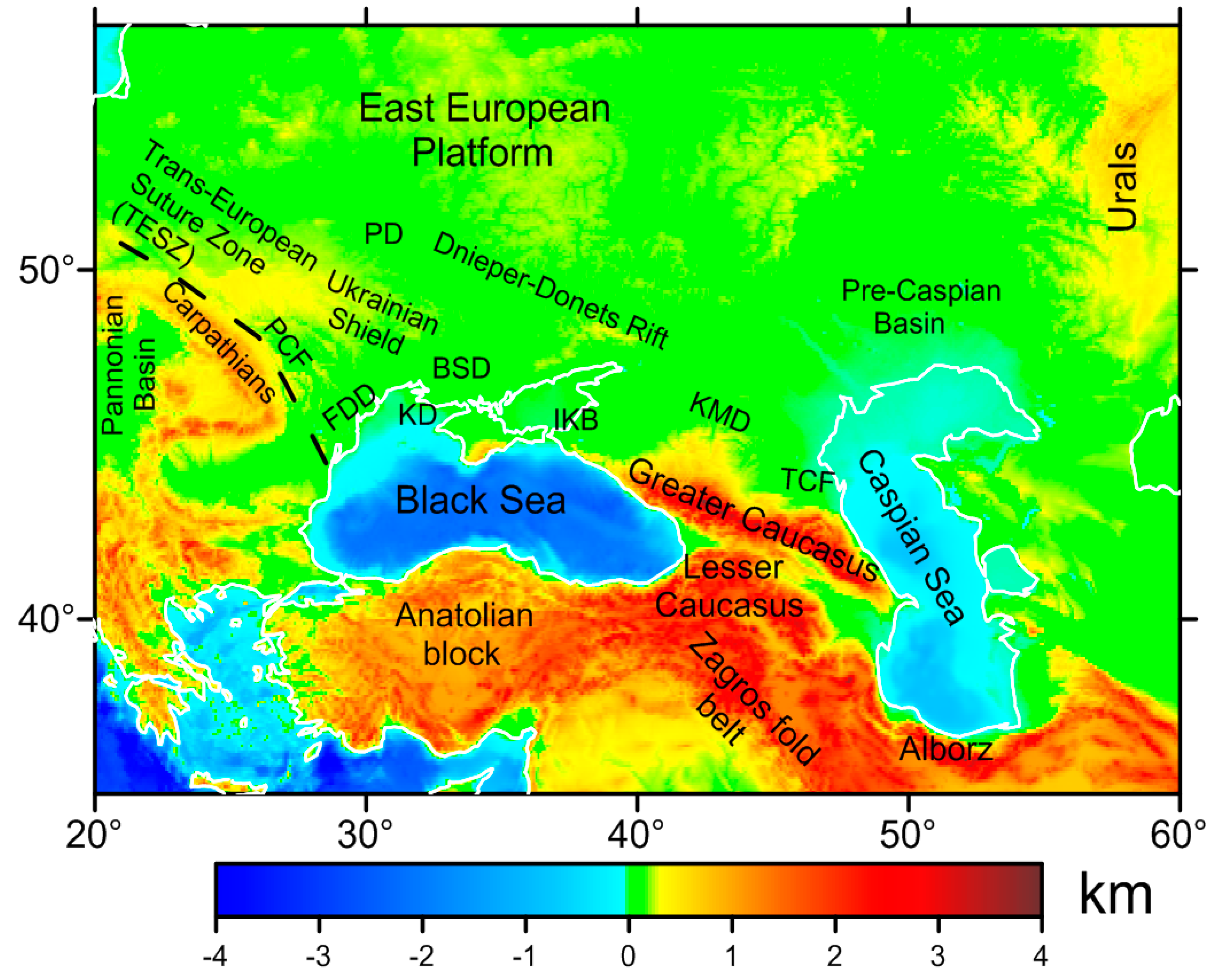
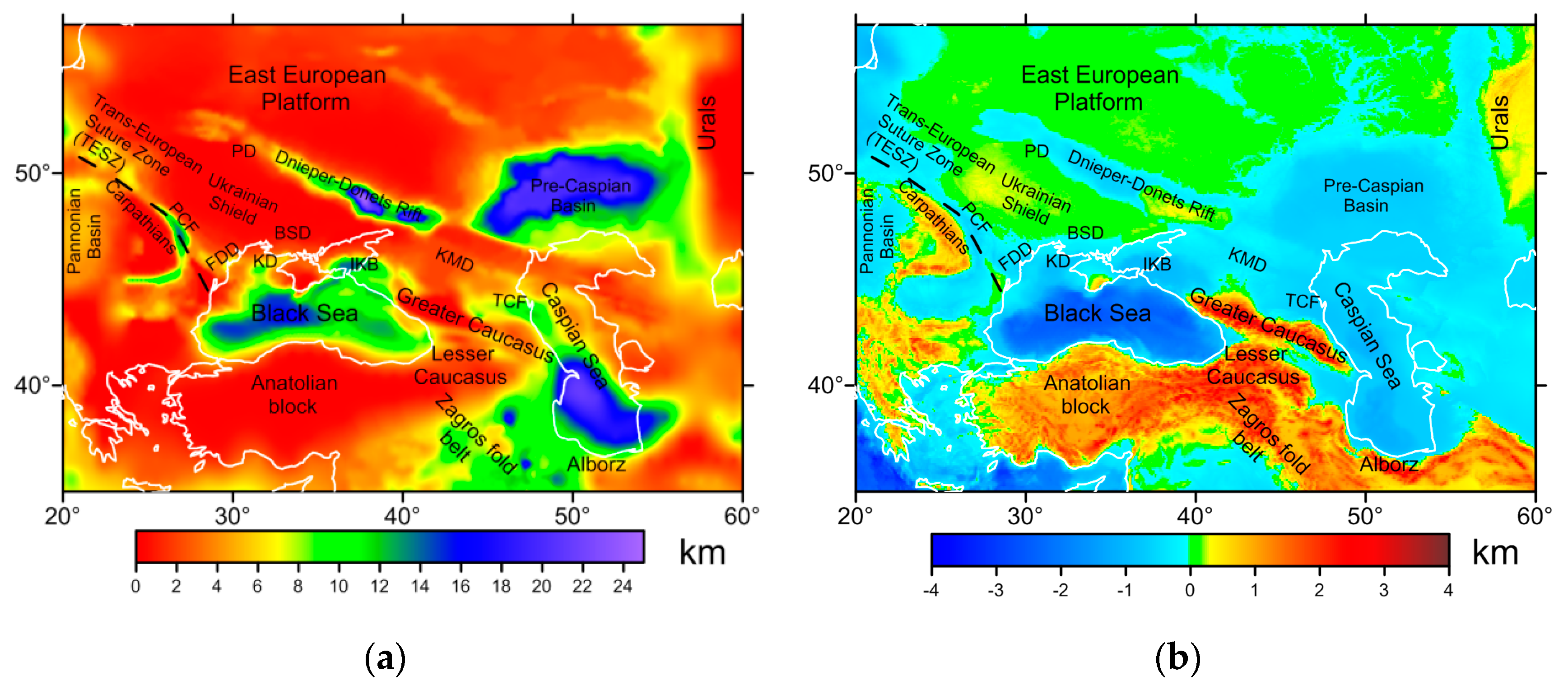
2.1. Sedimentary Basins in the Study Area: Origin and Structure

The study area includes the southern part of the EEP, Scythian plate and part of the Alpine-Mediterranean fold belt (the Caucasus and East Carpathians). The tectonic history of this area represents a long period from the pre-Riphean (more than 1600 MA), when the ancient crystalline basement of the East European Platform was formed, to the Miocene with the formation of the Greater Caucasus and the Black Sea depression (as a part of the Alpine Mediterranean fold belt). Most of the Scythian plate, except of its northwestern, southwestern and southeastern margins, was located within the Sarmatian shield divided by the Riphean and partially Late Devonian rifts. The Scythian plate represents a vast region of the modern Pre-Caucasus area, where the orogenic processes in the Carboniferous formed the Paleozoic (Hercynian) basement. Further development of this area, associated with the Arabia-Eurasia plate collision, resulted in formation of the extensive depressions that later evolved into sedimentary basins. Here we provide a description of the main sedimentary basins in the study area (Figure 1). For convenience, we use the abbreviations from this figure.

The Dnieper–Donets basin was initially formed as an ancient rift. Recent paleotectonic reconstructions [15] indicate that the development of the Dnieper–Donets depression included different stages. Initially, the riftogenesis was induced by mantle activity in the Late Devonian with simultaneous sedimentation under the conditions of marine transgression and subsequent regression. The next sedimentation stage was related to another marine transgression in the Middle Carboniferous. The deep depression in the southeastern part of the Dnieper–Donets basin was also developed in the Late Devonian—Early Carboniferous.

The Pripyat depression (PD) evolved almost simultaneously with the Dnieper–Donets basin on its west end in the Late Hercynian [16]. At that time, the terrigenous and carbonate rocks accumulated during the Devonian and Carboniferous with total thickness of 425 m above the existing Late Proterozoic (Riphean and Vendian) terrigenous deposits. Next, during the Early and Middle Carboniferous, the carbonate-terrigenous and coal-bearing deposits were accumulated with the total thickness 170–400 m. In the Late Carboniferous, the regional rise of the territory occurred completing the rifting process [17].

The Caspian basin is one of the largest sedimentary basins in the study area. The northern part of the basin is a part of the Scythian plate, and the southern one is associated with the Alpine-Mediterranean Cenozoic fold belt region. The sea basin within the present Caspian Sea appeared in Paleozoic, its shoreline has changed many times since then as a result of repeating transgressions and regressions which continue to this day due to climate changes [18]. Five main crustal blocks are defined within this region [19]: The North Caspian Basin (that is a part of the Pre-Caspian depression), the Middle Caspian Basin, the Apsheron Sill (separating the northern and middle Caspian basins), the Mangyshlak Sill (separating the middle and south Caspian basins) and the South Caspian Basin. Recent studies have shown that the rapid accumulation of sediments occurred within the South Caspian happened during the Mesozoic–Paleogene time. According to the existing maps, the thickness of sediments in the South Caspian increases from the north to the south, although this conclusion is not verified by seismic data.

The Pre-Caspian basin (PCB), sometimes referred as the North Caspian basin, is one of the deepest basins in the world, having more than 20 km sediments in the central part. Being a part of the East European Platform, the basin is bordered by the Uralides and the Northern Ustyurt Block in the east and by the Karpinsky rift in the southwest. The underlying basement represents either oceanic or thinned continental crust likely affected by several rifting processes between the Riphean and the Triassic. The thickness of the crust is still disputable and depends on interpretation of the high velocity layer at the base of the crust [20]. Despite being explored for about 100 years, the PCB’s structure is still poorly studied. There are several hypotheses concerning the origin of the basin, with the predominant one suggesting that the basin originated as a pre-Late Devonian rift. The deepest sediments of the PCB can be of either Riphean or Devonian origin, but the oldest rocks found in wells are of the Early and Middle Devonian age. According to existing seismic profiles, there exist three major layers constituting the basin: The subsalt, salt (Lower Permian) and upper layers. The sediments forming the subsalt layer differ in the central part of the basin and on its margins [21].

The Manych (Kuma-Manych) depression (KMD) is located at the border between the EEP and Scythian plate; it was formed within the fault zone that existed from the very beginning of the plate history. The KMD consists of a number of narrow en-echelon basins formed in compression environment during the continental plate collision. According to a long-standing hypothesis, the KMD is an ancient strait between the basins of the future Caspian and Black seas. Modern studies [22] confirm the existence of even four Pleistocene straits.

The origin of the Black Sea basin, adjoined to the Alpine-Mediterranean belt in the south, is still a subject of discussions. Its central part, which is about 15 km thick, overlays a suboceanic crust (~25 km) and was formed during the Paleozoic–Cenozoic [23]. The structure of the eastern part is nearly symmetrical, while the Western Black Sea Basin is characterized by remarkable asymmetry. Both Western and Eastern Black Sea basins have an oceanic or highly extended continental crust; they are separated by the Andrusov and Arkhangelsky ridges with a continental crust. Nikishin et al. [24] concluded that the Eastern Black Sea Basin was originated through rifting along an Early Cretaceous volcanic arc.

The Karkinit depression (KD) is located at the Black Sea border on the western coast of the Crimea Peninsula. However, being a part of the northwestern shallow water area of the Black Sea, the Western Crimea shelf has its own history and is different from the northwestern shelf of the Black Sea. The depression was formed on an ancient (pre-Riphean) deep fault [25] and is characterized by large thickness of the Cretaceous and Paleocene deposits. The overall thickness of sediments is about 6–7 km.

The Indolo-Kuban basin (IKB) was developed as a depression in the front of the plate collision belt. The depression extends from the Indol river to the east along the edge of the eastern part of the Mountainous Crimea, along the Kerch Peninsula to the Sea of Azov and then in the Pre-Caucasus towards the Kuban river delta. Geophysical data indicates that the depression, filled with thick sediments, is narrow and asymmetrical. In its western part (the Indol basin) the total strata thickness is about 4, 5 km; while in the central part (north of Kerch) the sediments are 10–13 km thick. In the eastern part of the basin the sedimentary thickness is approximately 3 km. The Indolo-Kuban basin is usually considered as a part of the large Azov-Kuban basin filled with Cretaceous to Cenozoic sediments [26].

The Terek–Caspian foredeep (TCF) is also related to the continental plate collision, being a foredeep of the East Greater Caucasus filled mainly with Meso-Cenozoic sediments with a Hercynian basement [27]. The southern part of the TCF experienced an intense subsidence due to the Stavropol uplift in Pliocene that separated the Indolo-Kuban (Azov-Kuban) and Terek–Caspian basins. The upper layer consists of the marine and continental Upper Pliocene and Quaternary deposits, mostly represented by ancient and modern alluvial river sediments.

The Black Sea Depression (BSD), adjacent to the Black Sea basin and the southern part of the EEP, is located at the north border on the Ukrainian Shield. According to most researchers, the formation of the depression began at the end of the Early Cretaceous (about 110 MA) as a result of subsidence of the southern slope of the Ukrainian Shield from the Late Mesozoic to Cenozoic. The basement underlying the Meso-Cenozoic layers consists of Precambrian and Epihercynian blocks separated by troughs. The thickness of the upper Cretaceous and Paleogenic deposits reaches is about 800 m in the northern part and up to 8–10 km in the southern part [28].

The Fore–Dobrogea depression (FDD) is located along the southwestern edge of the East European Platform next to the Black Sea depression and the Trans-European Suture Zone (TESZ). This depression is characterized by a complex heterogeneous structure of the basement. The underlying Proterozoic crystalline basement is overlapped by another Vendian–Devonian folded basement structure, in which a paleorift was formed. The sediments are represented by approximately 3 km of Middle Jurassic-Early Cretaceous rocks [29].

The Pre-Carpathians foredeep (PCF) is also characterized by structurally heterogeneous basement. In its southeastern (near the Dobrogea mountains) and northwestern parts the basement is Hercynian, and in the central part on the southwestern slope of the EEP it is older (Paleozoic) [30]. The inner (northeastern) zone of the foredeep is filled with dislocated sediments of the Cretaceous–Paleogene flysch and the Lower Miocene molasse–saliferous rocks. The outer (southeastern) zone is represented by the Upper Miocene sediments on the Jurassic and Cretaceous deposits. The thickness of the sediments is from 3 to 6 km. Some geological studies indicate that the Pre-Carpathians foredeep is a part of the larger sedimentary basin stretching for more than 1300 km from Austria to Romania and that the Pre-Carpathian foredeep developed as a peripheral foreland basin related to the moving Carpathian front during the early to middle Miocene [31].

The overview of the sedimentary basins in the study area shows that they represent a natural record of various tectonic processes shaped the area through time. Therefore, improvement of our knowledge about their structure is essential for understanding of these processes.

2.2. Method

Sediments are usually less dense than surrounding crystalline rocks, therefore, gravity data were often used for studying of sedimentary basins. Commonly, the isostatic gravity anomalies are used for these purposes. In these anomalies, the effect of deep density heterogeneity (e.g., of the Moho variations and density variations in the subcrustal layers), which dominate in the Bouguer gravity anomalies, is largely reduced, e.g., [32,33]. It was shown that the isostatic model, which is used for this correction, should include two basic parameters, namely the average depth to the compensating density anomalies, successfully approximated by the depth to the Moho, and flexural rigidity of the lithosphere. The last parameter controls transition between the local and regional isostatic compensation, it is directly related to the effective elastic thickness (EET) of the lithosphere [34]. Both parameters can be determined a-priory by independent methods. Therefore, the isostatic anomalies of the gravity field were widely used for studying of sedimentary basins, e.g., [35,36,37].

Unfortunately, the gravity effect of density variations within sedimentary basins might be substantially reduced (up to about 1 order of magnitude for wide basins), since these density anomalies are also isostatically compensated by deep masses and by elastic deformation of the lithosphere [38]. Long ago, it has been suggested to refine the full effect the upper crust and, in particularly, sediments by calculating a decompensative correction [38,39]. The efficiency of this correction has been demonstrated in many previous studies [38,40,41,42]. These authors employed essentially local isostatic compensation models (chiefly Airy). It has been demonstrated that ignoring flexural rigidity of the lithosphere may principally bias the results. Later on, Kaban et al. [13] and Haeger and Kaban [14] have improved this method to account for the EET of the lithosphere. It is also used in the present study. Therefore, the method applied in this paper consists of two principal steps. In the first step, we determine the isostatic correction and calculate the isostatic gravity anomalies. In the next step, the decompensative correction and decompensative gravity anomalies are calculated. These anomalies are used to correct an initial density model of the sedimentary cover.

The isostatic correction in the spectral domain can be calculated according to [43] as:

Δg_ic (k_x, k_y) = G_is (k_x, k_y)·t_adj (k_x, k_y) = −2 πGρ C·exp (−k·M)…t_adj (k_x, k_y),

(1)

where M is the depth to the Moho, $k=\sqrt{k_x^2+k_y^2}$ is the wavenumber, k_x = 2π/λ_x and k_y = 2π/λ_y, G is the gravitational constant, t_adj is the adjusted topography, which is introduced in the sea area to equalize the bathymetry (t_b) and topography variations for the constant density of the topography ρ. In the present study, the adjusted topography is also corrected for the initial model of the sedimentary cover:

$${\mathrm{t}}_{\mathrm{adj}}={\mathrm{t}}_{\mathrm{b}}-\frac{{\mathsf{\rho }}_{\mathrm{w}}}{\mathsf{\rho }}{\mathrm{t}}_{\mathrm{b}}-\frac{{\mathsf{\rho }}_{ }-{\mathsf{\rho }}_{\mathrm{s}}}{\mathsf{\rho }}{\mathrm{t}}_{\mathrm{s}},$$

(2)

where ρ_w = 1.03 g/cm³ is the water density, ρ_s and t_s are the vertically averaged density and thickness of sediments according to the initial model.

The parameter C determines the transition between the local and regional compensation (C = 1 for essentially local) depends on the wavenumber and EET (T_e), e.g., [44]:

C = Δρg/(k⁴D + Δρg),

(3)

where EET (T_e) is the effective elastic thickness of the lithosphere, D = E(T_e)³/[12(1 − ν²)] is the flexural rigidity, E is the Young modulus, ν is the Poisson ratio, Δρ is the average difference of the density of topography and the upper mantle material, and g is the gravitational acceleration.

It is impossible to use directly Equation (1) since both M and T_e vary in space. Instead, we apply a Green’s function approach [45,46,47]. In these publications, the authors have shown that this method works well for such kinds of problems. The Green’s function (G_is) is determined for each combination M and T_e by the inverse Fourier transform of the terms applied to t_adj in Equation (1). Then, the isostatic correction is calculated as a convolution of the adjusted topography and corresponding Green’s functions in a sliding window, giving the isostatic anomalies:

$$\mathsf{\Delta }{\mathrm{g}}_{\mathrm{i}}\left({\mathrm{x}}_0,{\mathrm{y}}_0\right)=\mathsf{\Delta }{\mathrm{g}}_{\mathrm{b}}\left({\mathrm{x}}_0,{\mathrm{y}}_0\right)+\underset{-1250\mathrm{km}}{\overset{1250\mathrm{km}}{{\displaystyle \iint }}}{\mathrm{t}}_{\mathrm{adj}}\left({\mathrm{x}}_0+\mathrm{x},{\mathrm{y}}_0+\mathrm{y}\right)\mathsf{·}{\mathrm{G}}_{\mathrm{is}}\left(\mathrm{x},\mathrm{y}, \mathrm{M},{ \mathrm{T}}_{\mathrm{e}}\right)\mathrm{dxdy}$$

(4)

where $\mathsf{\Delta }{\mathrm{g}}_{\mathrm{b}}\left(\mathrm{x},\mathrm{y}\right)$ is the Bouguer gravity anomaly. The convolution radius is 1250 km, consequently, the study area was extended correspondingly to avoid boundary effects.

The decompensative correction (Δg_dc) for the isostatic anomalies can be calculated following [13]:

$$\mathsf{\Delta }{\mathsf{g}}_{\mathrm{dc}} \left(kx,ky\right)= \frac{1}{\exp \left(\mathrm{k}\mathsf{·}\mathrm{M}\right)/\mathrm{C}- 1 }\mathsf{·}\mathsf{\Delta }\mathrm{gi}\left(kx,ky\right),$$

(5)

where Δg_i are the isostatic anomalies. The initial expression formulated in [38,39] has been expanded to take into account elastic support of the lithosphere [13]. Δgdc exponentially rises to infinity with increasing of the wavelength. Cordell et al. [38] suggested reducing it after some predefined wavelength (λ₀) by applying a high-pass filter. This limitation should not bias the result since we do not consider continental-wide structures. In this study we choose the boundary wavelength equal to 2500 km following numerical tests in [13]. The decompensative correction is estimated in the same way as the isostatic anomalies by applying the Green’s function approach (Equation (4)). The decompensative anomalies are calculated as a sum of the isostatic gravity anomalies and decompensative correction.

2.3. Isostatic and Decompensative Gravity Anomalies

2.3.1. Initial Data

For computation of the isostatic and decompensative gravity anomalies we employ five principal data set: Bouguer gravity anomalies, topography, initial model of the sedimentary cover (thickness and density), depth to the Moho based on seismic determinations and EET of the lithosphere. All these grids have resolution of 5′ × 5′, they have been obtained in previous studies and summarized in [48]. The Bouguer gravity anomalies (Figure 1) are calculated from the EIGEN-6c4 model [12], which is based on a combination of the recent satellite missions (chiefly GRACE and GOCE) and surface/airborne observations. The resolution of this model is 2190 spherical harmonics degree/order, which approximately corresponds to 5′ × 5′ in space. The topography correction is calculated using the ETOPO-1 data [49]. The density of the topography is assumed to be 2.67 g/cm³, and of the water—1.03 g/cm³. The calculation technique accounts for sphericity of the Earth, it is explained in details in [43]. The effect of the initial density model of the sedimentary cover is also removed from the Bouguer gravity anomalies [48]. The residual field is shown in Figure 2b.

The initial model of sediments (thickness) is shown in Figure 3a. For most of the study area, we used the compilation of Kaban [3], which was supplemented by the data of Kaban et al. [43] for the Anatolian block, part of the Lesser Caucasus and Zagros fold belt. These data have been also used for determination of the adjusted topography (Equation (2), Figure 3b). It represents a result of numerical “densification” of water and sedimentary tocks to the standard density of topography (2.67 g/cm³). It is visible that after this procedure, vast areas in the continental part expose negative topography.

For the Moho boundary (Figure 4a), we used the same model as in [48]. It is based on the EuCRUST-07 data [50], which were supplemented in the eastern part by the model presented in [51]. The effective elastic thickness (Figure 4b) used in this study is calculated with the fan wavelet coherence technique [48].

2.3.2. Decompensative Correction

The isostatic correction computed from the adjusted topography (Figure 3b) is shown in Figure 5a. Mostly mid-wavelength are dominated in this field as the effect of small-scale compensation is largely reduced by the relatively large compensation depth and, especially by the high values of EET (Figure 4). Adding of this correction to the Bouguer gravity anomalies with the removed effect of sediments (Figure 2b) results in the isostatic gravity anomalies. At the long wavelengths these anomalies are still dominated by the dynamic effects induced by the mantle convection [52,53]. However, it was demonstrated in the above papers that this effect can be easily reduced by applying a gauss-type filter with the boundary wavelength (half amplitude) about 2500 km. The short wavelengths are not biased by this procedure since the spectrum of the isostatic anomalies usually has relative minimum in the transition wavelengths. The residual isostatic anomalies are shown in Figure 4b.

Relatively small-scale anomalies are generally presented in the residual isostatic field. This is a result of partial isostatic compensation of near-surface density anomalies as was suggested above. We further apply the decompensative correction to restore the full effect of the shallow subsurface structures.

The decompensative correction for the isostatic gravity anomalies is shown in Figure 6a. It is relatively insignificant in the areas with high values of EET exceeding 50 km since most of the isostatic compensation is provided by long-wavelength elastic deformations of the lithosphere. However, in other areas (e.g., in the Black Sea and Dnieper–Donetsk Rift) it is significant and reaches the amplitudes ±50 mGal (Figure 6a).

The final decompensative gravity anomalies are shown in Figure 6b. Their amplitude varies within the range ±135 mGal, which is already comparable with the effect of the initial density model of the sedimentary cover. In further chapters these anomalies are interpreted with respect to correction of this model.

3. Results

The decompensative gravity anomalies have been employed to refine the initial model of the sedimentary cover. Initially, the whole anomaly has been attributed to the sedimentary cover. The gravity anomalies could be equally determined by changes of thickness and density of sediments. It is impossible to determine a priori of which factor dominates in each specific case. In general, we consider them as equally important and assume that half of the decompensative anomaly is caused by a change of the thickness and half—by density:

$$\left(\mathrm{S} + \mathsf{\Delta }\mathrm{S}\right)\mathsf{\Delta }{\overline{\mathsf{\rho }}}_{\mathrm{S}}= \mathsf{\Delta }\mathrm{S}\left(\mathsf{\Delta }{\overline{\mathsf{\rho }}}_{\mathrm{ini}}+\mathsf{\Delta }{\overline{\mathsf{\rho }}}_{\mathrm{S}}\right)$$

(6)

where S is the initial thickness of sediments, ∆S is its change, $\mathsf{\Delta }{\overline{\mathsf{\rho }}}_{\mathrm{ini}}$ is the initial density of sediments (vertically averaged relative to the standard value 2.7 g/cm³) and $\mathsf{\Delta }{\overline{\mathsf{\rho }}}_{\mathrm{S}}$ is the density perturbation.

Afterwards, several limitations were applied to the model to keep it realistic:

• It is supposed that the areas without sediments or with very low amount of them are determined reliably in the initial model. Therefore, we do not apply the correction to the areas where the thickness is less than 0.25 km.
• It is assumed that sedimentary thickness should not exceed 25 km, the limit, which is determined based on existing seismic studies.
• The maximal reduction of the sedimentary thickness is limited to 0.75 of the initial one.
• The final density of sediments (averaged with depth) should be within the range 1.9–2.8 g/cm³, which is consistent with experimental data, e.g., [54].

Therefore, the condition (6) is not always met and in some cases only part of the decompensative anomalies can be explained by modification of the initial model of sediments. In the last case, the rest is attributed to the top layer of the crystalline crust. The inversion for changes of the sedimentary thickness and density was performed in an iterative procedure. First, it is estimated for the 1D case as the simple Bouguer correction by fitting the equation:

$$\mathsf{\Delta }{\mathsf{g}}_{\mathsf{d}} = 2\mathsf{\pi }\mathrm{G} \left[\left(\mathrm{S} + \mathsf{\Delta }\mathrm{S}\right)\mathsf{\Delta }{\overline{\mathsf{\rho }}}_{\mathrm{S}}+\mathsf{\Delta }{\overline{\mathsf{\rho }}}_{\mathrm{ini}} \mathsf{\Delta }\mathrm{S} + \mathsf{\Delta }{\overline{\mathsf{\rho }}}_{\mathrm{uc}}{\mathsf{h}}_{\mathrm{uc}}\right]$$

(7)

where h_uc = 15 km is the top layer of the crystalline crust and $\mathsf{\Delta }{\overline{\mathsf{\rho }}}_{\mathrm{uc}}$ is the density change within this layer. The third term appears only when it is not possible to fit the decompensative anomaly solely by modification of the sedimentary layer parameters due to the above limitations. In the next step, the gravity effect of the modified mode was estimated by using a 3D modelling technique on the sphere [43]. The difference with the original decompensative anomalies was used then to estimate corrections for the initial model. The convergence is reached very fast (usually in the second step) because 3D effects are not significant for relatively small depths.

The obtained corrections and final map of the sedimentary thickness are shown in Figure 7. The correction is quite significant in many areas and spans within the range −11–+8.5 km (Figure 7a). Consequently, the differences of the final map (Figure 7b) with the initial one (Figure 3a) are also significant. We will discuss them in the following section.

In the same way, the corrections for the initial density of sediments were estimated (Figure 8a). It spans in the range from −0.6 g/cm³ to +0.6 g/cm³. The final map of the averaged density is demonstrated in Figure 8b. It should be noted that the average density of sediments does not directly relate to their gravity effect. The last one is also determined by thickness. Density of sediments rapidly increases with depth due to compaction, e.g., [55], therefore, the difference between the density of thick sediments and upper crust is usually small or moderate. Nevertheless, they might induce a large gravity anomaly. More discussion is presented in the following section.

It should be noted that the obtained results are rather qualitative than quantitative. First of all, there exists obvious ambiguity between the effects of density and thickness variations of the sedimentary cover. Second, part of the decompensative anomalies may be induced by density variations in the uppermost crystalline crust, although their effect is likely remarkably less than the effect of sediments, e.g., [54,56]. Therefore, in the following discussion we consider general tendencies but not specific values.

4. Discussion

In this section we discuss the corrected thickness and density maps for major sedimentary deposits within the study area. Very principal changes have been obtained for the Black Sea and adjacent basins. The sedimentary basins in the western and eastern parts of the Black Sea are already different in the initial model; the eastern basin is much shallow than the western one (Figure 3a). In the corrected model we found also a strong difference between the northern and southern parts of the East Black Sea (Figure 7). The deepest part of the western Black Sea basin is now shifted to the north and joined to the Indolo–Kuban basin. The upper part of the sedimentary cover of the Black Sea was extensively studied by seismic methods (CDP), which results have been summarized in [24,57,58]. The sedimentary map, presented in these papers, is characterized by a completely opposite pattern; the northeastern part of the basin is much shallow than the southeastern part. However, the deepest boundary shown in these studies is represented by the top of Cretaceous sediments, which is considered as basement. The density of these sediments might be relatively low even if the seismic velocities are normal, e.g., [59]. Therefore, we have to conclude that the effect of the Cretaceous and possibly even older layers is also significant and may not be ignored in a complete model.

The density changes, obtained for the Black Sea basins are not significant because the total sedimentary thickness is quite large (Figure 8). North of the Black Sea, some gradual density changes from north to south have been revealed for the Black Sea depression. These changes are mainly due to the differences in sedimentary types and their age. The density gradient (1.8 to 2.25 g/cm³, approximately) agrees with the presence of more dense Eocene, Jurassic, and even Paleozoic rocks underlying the upper Neogenic layer represented by carbonate, sandy-clayey and coarse-detrital Miocene and Pliocene deposits in the southern and southwestern parts of the basin. It is clear that the Northwestern Black Sea shelf combines the structures of three tectonic regions: The EEP, the Scythian plate and the Mountain Crimea folded belt. In the new model, the Karkinit depression basin appears to be more isolated from the rest of the Western Black Sea basin, although its depth remains the same. The new model proves that the Karkinit depression developed on a previously existing deep fault.

The eastern part of the Indolo-Kuban basin continues in the Pre-Caucasus in latitudinal direction and is characterized by nearly constant density (about 2.4–2.45 g/cm³), joining the western part of the similar Terek–Caspian basin. The Kuma–Manych depression is also clearly revealed as a sublatitudinal zone with the density about 2.4 g/cm³. However, both models for this structure (the initial and the new ones) show similar thickness with its slight increase to the southeast while approaching the Caspian. The Greater Caucasus is clearly divided into two parts, which are characterized by remarkably different structure of the lithosphere, e.g., [60]. For the West Greater Caucasus we did not obtain any significant correction, which demonstrates that the initial model without sediments works well. Contrary to the western part, the East Greater Caucasus is characterized by extensive sedimentary layers with the total thickness reaching 2.5 km in the initial model (Figure 3a). However, their density was previously reported as rather high. According to the density model summarized in [61], the average density of the Paleogenic rocks is 2.23 g/cm³, of the Cretaceous—2.48 g/cm³ and of the Jurassic and older—2.62 to 2.72 g/cm³. Therefore, the top of the Cretaceous was already considered as a basement since the density of the lower layers is not much different from the crystalline crust. For this structure, the decompensative anomaly reaches −95 mGal, which evidences that the gravity effect of the sediments in the East Greater Caucasus is much stronger than in the initial model. The corrected sedimentary thickness reaches 6–7 km in some places (Figure 7), while their average density is also significantly reduced (Figure 8). This means that the relatively older layers starting from the Cretaceous to at least Paleozoic ones should be considered as a part of a relatively low-dense sedimentary cover. For the Kura intermountain basin, which is located south of the East Greater Caucasus, the corrections are low supporting the initial model. For the pre-Caucasus foredeeps, a significant correction has been obtained in the west for the western part of the Indolo-Kuban basin, which is deepened considerably (Figure 7).

A very significant correction has been obtained for South Caspian and for the Terek–Caspian foredeep. In the initial model, the deep basin with the sedimentary thickness up to 22 km extends to the southern border although its southern part is not well constrained by seismic data. In the corrected model, it is shifted to the north close to the Apsheron Trough with the thickness up to 25 km. Several strong earthquakes are associated with the deepest part of the basin, e.g., [60], which confirms that its formation is directly related to the collision of the Arabian and Eurasian plates, e.g., [48]. In the southern part of the South Caspian basin, the sedimentary thickness is significantly reduced, likely following the inclined plate subducting to the north. The new model also shows large sedimentary thickness (about 20 km) in the Terek–Caspian foredeep (Figure 7b), in an isometric zone referring to its deepest axial part. This agrees with the exploration drilling results on the Terek-Kuma lowland site [27] that revealed the Hercynian basement top at a depth of more than 10 km. The Terek–Caspian foredeep continues into the Caspian Sea having the average density 2.5–2.55 g/cm³ and approaching the density values 2.6–2.7 g/cm³ only in the northern border of the South Caspian block. This may evidence for a closer relation of the foredeep to the South Caspian Basin than in the initial model, in which the Terek–Caspian basin is only 12–14 km deep. It might be also assumed that this deepest part of the foredeep existed since the Late Paleozoic as a part of the South Caspian. Both new thickness and density models for this basin agree with the heat flow map of Mansouri and Zui [19] displaying that the Terek–Caspian foredeep and the Central Caspian are both characterized by low values of the heat flow.

In the Pre-Caspian (or North Caspian) basin, the thickness of sediments is significantly reduced in its eastern part. Some of regional maps also show reduction of the sedimentary thickness in the eastern part of the basin [20]; however, the origin of this feature is still under debates. As was mentioned in Section 2, there exists heterogeneity of the PCB subsalt layer from the edges to the center of the basin: The shallow-shelf carbonate formations, which contain various reefs and alternate with clastic wedges, compose the subsalt sequence at the basin margins. Towards the center, these rocks transform into the deep-water anoxic black shales and turbidites [21]. The next layer, represented by the Lower Permian saliferous series, was deformed into domes during the Late Permian–Triassic. Above the saliferous series, there exists a layer predominantly consisting of clastic rocks up to several kilometers thick in depressions between the salt domes. The low-thickness (2–4 km) zone can correspond to the Aralsor gravity maximum (about 50 mGal on the Bouguer anomaly map on Figure 2a and approximately 200 mGal in the residual gravity field, Figure 2b). This structure can be a result of the complicated tectonic history of the basin and of the evolution and closure of the Paleozoic Ural ocean basin, when an active continental margin existed in the east and southeast of the modern Pre-Caspian depression [62].

The average density of sediments within the Dnieper–Donets Rift is already high in the initial model and in some places exceeds the normal density of the upper crystalline crust (up to 2.75 g/cm³). Our analysis demonstrates that it should be even higher in the northern part, while the insignificant decompensative anomalies in the southern part show that the initial model is satisfactory. The southeastern part of the Dnieper–Donets basin developed in the conditions of abyssal depression, as indicated by sedimentary formations in the Late Devonian–Early Carboniferous. According to [15], significant differences between the riftogenesis processes in the northwest and the southeast of the Dnieper–Donets depression were probably caused by different contribution of the mantle. This can be a possible explanation of such density contrast in the model. The new model for the Pripyat depression doesn’t also display any significant changes.

The depth of the Pre-Carpathians foredeep is only slightly modified in the corrected model by some redistribution of sediments between its northern and southern parts. The deepest depression is now located at the southern flank. This is likely associated with more active tectonic processes and higher horizontal stresses in the north-south direction originated from the collision of Arabia and Eurasia than those related to the Carpathian front movement in the east-west direction. The changes for the Fore–Dobrogea depression are insignificant in the new model.

5. Conclusions

In this study we present a new model of the sedimentary cover for the southern part of the East European Platform (EEP) and some adjoining structures. This model, which implies thickness and density of sediments, is based on the analysis of the decompensative gravity anomalies. Up to now, most of the gravity studies were employed the Bouguer or isostatic gravity anomalies for investigation of the upper crust structure. Our study confirms that ignoring the effect of the deep masses that compensate near-surface load may principally bias the result. The decompensative correction computed for the study area spans within ±50 mGal, which is about half of the amplitude of the initial isostatic anomalies. The resulting decompensative gravity anomalies have been used for modification of the initial model of the sedimentary cover.

The analysis of the new model for the southern part of the East European Platform, Greater Caucasus and adjacent areas shows that in general it better matches to the modern view on the geology and tectonics of this region, despite of some differences with a number of studies. It is worth noting that several principal corrections have been obtained for density and thickness of several deep basins, whose structure has been debated for decades. In particular, the new information on the Black and Caspian Sea basins has been obtained. In the new model we also found a strong difference between the northern and southern parts of the East Black Sea, however the deepest basin in the western part is located in the north and joined to the Indolo–Kuban basin. This conclusion contradicts to previous studies, which defined basement as a top of the Cretaceous rocks, and demonstrates that they, and possibly even older layers, should be included in a complete model.

Another principal finding is that metamorphosed sediments in the East Greater Caucasus are characterized by remarkably less densities than it was suggested in the initial model, in which they are almost indistinguishable from the crystalline rocks of the Western Greater Caucasus already at rather shallow depths. Significant corrections are also obtained for the foredeep of the East Greater Caucasus, the Terek–Caspian depression. In the new model it is nearly jointed with the deepest part of the South Caspian depression. In the corrected model, the maximum depth to basement is shifted from its central part to the north close to the Apsheron Trough with the thickness of sediments up to 25 km.

In the Pre-Caspian (or North Caspian) basin, the thickness of sediments is significantly reduced in the eastern part compared to the initial model. This reduction agrees with several recent seismic studies and is likely related to the former tectonic activity at the active continental margin of the Paleozoic Ural ocean in the east and southeast of the modern Pre-Caspian depression basin.

Therefore, the method based on the analysis of the decompensative anomalies can reveal hidden features of the sedimentary cover. It doesn’t provide a comprehensive 3D model of sediments, some issues remain unresolved. In particularly, the resolution of the initial gravity field might be insufficient due to the lack of dense ground networks. However, the revealed anomalies may indicate potential areas, which can be investigated in details, not only for fundamental purposes but also in applied geology, including mineral deposits prospecting and engineering.

References

1. Artemieva, I.M.; Thybo, H.; Kaban, M.K. Deep Europe today: Geophysical synthesis of the upper mantle structure and lithospheric processes over 3.5 By. In European Lithosphere Dynamics; Gee, D., Stephenson, R., Eds.; Geological Society London Memoirs: London, UK, 2006; Volume 32, pp. 11–41. [Google Scholar]
2. Bur’yanov, V.B. The Gravity Field and Density Models of the European Tectonosphere. Int. Geol. Rev. 1985, 27, 1021–1027. [Google Scholar] [CrossRef]
3. Kaban, M.K. A gravity model of the north Eurasia crust and upper mantle: 2. The Alpine-Mediterranean fold belt and adjacent structures of the southern former USSR. Russ. J. Earth Sci. 2002, 4, 19–33. [Google Scholar] [CrossRef] [Green Version]
4. Yegorova, T.P.; Starostenko, V.I. Lithosphere structure of European sedimentary basins from regional three-dimensional gravity modelling. Tectonophysics 2002, 346, 5–21. [Google Scholar] [CrossRef]
5. Bronguleev, V.V. (Ed.) Map of the Pre-Riphean Basement Upper Surface Depth of the East-European Platform; Scale 1:5,000,000; MinGeo: Moscow, Russia, 1986. (In Russian) [Google Scholar]
6. Artemieva, I.M. Dynamic topography of the East European craton: Shedding light upon lithospheric structure, composition and mantle dynamics. Glob. Planet. Change 2007, 58, 411–434. [Google Scholar] [CrossRef] [Green Version]
7. Bronguleev, V.V. On the compilation of maps of structural correspondence between surface and basement relief at the East European plate. Geomorfologia 1977, 4, 44–52. (In Russian) [Google Scholar]
8. Giese, P.; Pavlenkova, N.I. Structural Maps of the Earth’s Crust for Europe. Izv. Earth Phys. 1988, 24, 767–775. [Google Scholar]
9. Hurtig, E.; Cermak, V.; Haenel, R.; Zui, V. (Eds.) Geothermal Atlas of Europe; GeoForschungsZentrum Potsdam, Publication No. 1; Hermann Haack Verlags-Gesellschaft—Geographisch-Kartographische Anstalt: Gotha, Germany, 1992. [Google Scholar]
10. Gorbatikov, A.V.; Rogozhin, E.A.; Stepanova, M.Y.; Kharazova, Y.V.; Andreeva, N.V.; Perederin, F.V.; Zaalishvili, V.B.; Mel’kov, D.A.; Dzeranov, B.V.; Dzeboev, B.A.; et al. The pattern of deep structure and recent tectonics of the Greater Caucasus in the Ossetian sector from the complex geophysical data. Izv. Phys. Solid Earth 2015, 51, 26–37. [Google Scholar] [CrossRef]
11. Bulychev, A.A.; Sidorov, R.V.; Dzhamalov, R.G. Use of data of satellite system for gravity recovery and climate experiment (GRACE) for studying and assessment of hydrological-geohydrological characteristics of large river basins. Water Resour. 2012, 39, 514–522. [Google Scholar] [CrossRef]
12. Förste, C.; Bruinsma, S.L.; Abrikosov, O.; Lemoine, J.-M.; Marty, J.C.; Flechtner, F.; Balmino, G.; Barthelmes, F.; Biancale, R. EIGEN-6C4 the Latest Combined Global Gravity Field Model Including GOCE Data Up to Degree and Order 2190 of GFZ Potsdam and GRGS Toulouse; GFZ Data Services: Potsdam, Germany, 2014. [Google Scholar] [CrossRef]
13. Kaban, M.K.; El Khrepy, S.; Al-Arifi, N. Importance of the Decompensative Correction of the Gravity Field for Study of the Upper Crust: Application to the Arabian Plate and Surroundings. Pure Appl. Geophys. 2017, 174, 349–358. [Google Scholar] [CrossRef]
14. Haeger, C.; Kaban, M.K. Decompensative Gravity Anomalies Reveal the Structure of the Upper Crust of Antarctica. Pure Appl. Geophys. 2019, 1–14. [Google Scholar] [CrossRef]
15. Gonchar, V.V. Formation and sedimentary filling of the Dnieper-Donets depression (geodynamics and facies) in the light of new data of paleotectonic modeling. Geofizicheskii Zhurnal (Geophys. J.) 2018, 40, 67–94. [Google Scholar] [CrossRef] [Green Version]
16. Kirikov, V.P.; Verbitsky, V.R.; Verbitsky, I.V. Platform covers tectonic zoning: Case of the East European platform. Reg. Geol. Metall. 2017, 72, 15–25. (In Russian). Available online: https://vsegei.ru/ru/public/reggeology_met/content/2017/72/72_02.pdf (accessed on 14 July 2020).
17. Garetskii, R.G.; Aizberg, R.E.; Starchik, T.A. Pripyat Trough: Tectonics, geodynamics, and evolution. Russ. J. Earth Sci. 2004, 6, 217–250. [Google Scholar] [CrossRef]
18. Lebedev, S.A. Climatic variability of water circulation in the Caspian Sea based on satellite altimetry data. Int. J. Remote Sens. 2018. [Google Scholar] [CrossRef]
19. Mansouri, F.S.; Zui, V.I. Geothermal field and geology of the Caspian Sea region. J. Belarusian State Univ. Geogr. Geol. 2019, 1, 104–118. [Google Scholar] [CrossRef]
20. Brunet, M.-F.; Volozh, Y.; Antipov, M.; Lobkovsky, L. The geodynamic evolution of the Precaspian Basin (Kazakhstan) along a north–south section. Tectonophysics 1999, 313, 85–106. [Google Scholar] [CrossRef]
21. Ulmishek, G.F. Petroleum Geology and Resources of the North Caspian Basin, Kazakhstan and Russia; US Geological Survey: Reston, VA, USA, 2001. [CrossRef]
22. Svitoch, A.A.; Sobolev, V.M. Pleistocene straits of Manych (morphology, construction and development). Bull. Mosc. Univ. Ser. 5 Geogr. 2011, 4, 70–77. (In Russian) [Google Scholar]
23. Goncharov, V.P.; Neprochnov, Y.P.; Neprochnova, A.F. Bottom Topography and Deep Structure of the Black Sea Depression; Nauka: Moscow, Russia, 1972; pp. 131–134. (In Russian) [Google Scholar]
24. Nikishin, A.M.; Okay, A.I.; Tüysüz, O.; Demirer, A.; Amelin, N.; Petrov, E. The Black Sea basins structure and history: New model based on new deep penetration regional seismic data. Part 1: Basins structure and fill. Mar. Petrol. Geol. 2015, 59, 638–655. [Google Scholar] [CrossRef]
25. Myslivets, V.I.; Rimsky-Korsakov, N.A.; Korotaev, V.N.; Porotov, A.V.; Pronin, A.A.; Ivanov, V.V. Morphostructures and Sedimentary Cover Structure of the Inner Shelf of Western Crimea. Oceanology 2019, 59, 965–974. [Google Scholar] [CrossRef]
26. Assessment of Undiscovered Oil and Gas Resources of the Azov–Kuban Basin Province, Ukraine and Russia. USGS. 2010. Available online: https://pubs.usgs.gov/fs/2011/3052/pdf/fs2011-3052.pdf (accessed on 25 August 2020).
27. Abumuslimov, A.A.; Bankurova, R.U.; Alakhverdiyev, F.D. Features of the geomorphology of the Terek-Kuma lowland. Bull. Acad. Sci. Chechen Repub. 2013, 18, 72–76. [Google Scholar]
28. Volchegursky, L.F.; Garetsky, R.G.; Kiryukhin, L.G.; Muratov, M.V.; Raaben, M.E.; Freidlin, A.A.; Shlesinger, A.E.; Yanshin, A.L. Tectonics of the East-European Platform and Its Surroundings: A Digest; Nauka: Moscow, Russia, 1975; pp. 37–39. (In Russian) [Google Scholar]
29. Amashukeli, T.A.; Murovskaya, A.V.; Yegorova, T.P.; Alokhin, V.I. The deep structure of the Dobrogea and Fore-Dobrogea trough as an indication of the development of the Trans-European suture zone. Geofizicheskiy Zhurnal 2019, 41, 153–171. [Google Scholar] [CrossRef]
30. Arutyunova, N.M.; Afanasyev, Y.T.; Bagdasarova, M.V.; Bayrak, I.K.; Kalimullin, O.K.; Kornienko, G.E.; Korotkov, V.A.; Korotkova, M.K.; Kuvykin, Y.S.; Markova, E.V.; et al. Oil and Gas Content of Great Depths; Nauka: Moscow, Russia, 1980; pp. 26–28. (In Russian) [Google Scholar]
31. Oszczypko, N.; Krzywiec, P.; Popadyuk, I.; Peryt, T. Carpathian Foredeep Basin (Poland and Ukraine): Its Sedimentary, Structural, and Geodynamic Evolution. In The Carpathians and Their Foreland: Geology and Hydrocarbon Resources AAPG Memoir; Golonka, J., Picha, F.J., Eds.; American Association of Petroleum Geologists: Tulsa, OK, USA, 2006; Volume 84, pp. 221–258. [Google Scholar] [CrossRef]
32. Blakely, R.J. Potential Theory in Gravity and Magnetic Applications; Cambridge University Press Science: London, UK, 1995. [Google Scholar]
33. Simpson, R.W.; Jachens, R.C.; Blakely, R.J.; Saltus, R.W. A new isostatic residual gravity map of the conterminous United States with a discussion on the significance of isostatic residual anomalies. J. Geophys. Res. 1986, 91, 8348–8372. [Google Scholar] [CrossRef]
34. Burov, E.B.; Diament, M. The effective elastic thickness (Te) of continental lithosphere: What does it really mean? J. Geophys. Res. 1995, 100, 3905–3927. [Google Scholar] [CrossRef] [Green Version]
35. Langenheim, V.E.; Jachens, R.C. Gravity Data Collected along the Los Angeles Regional Seismic Experiment (LARSE) and Preliminary Model of Regional Density Variations in Basement Rocks, Southern California; U.S. Geological Survey Open File Report 96-682; U.S. Geological Survey: Reston, VA, USA, 1996. [Google Scholar] [CrossRef]
36. Jachens, R.C.; Moring, C. Maps of the Thickness of Cenozoic Deposits and the Isostatic Residual Gravity over Basement for Nevada; U.S. Geological Survey Open File Report 90-404; U.S. Geological Survey: Reston, VA, USA, 1990. [Google Scholar] [CrossRef]
37. Ebbing, J.; Braitenberg, C.; Wienecke, S. Insights into the lithospheric structure and the tectonic setting of the Barents Sea region from isostatic considerations. Geophys. J. Int. 2007, 171, 1390–1403. [Google Scholar] [CrossRef] [Green Version]
38. Cordell, L.; Zorin, Y.A.; Keller, G.R. The decompensative gravity anomaly and deep structure of the region of the Rio Grande rift. J. Geophys. Res. Solid Earth 1991, 96, 6557–6568. [Google Scholar] [CrossRef]
39. Zorin, Y.A.; Pismenny, B.M.; Novoselova, M.R.; Turutanov, E.K. Decompensative gravity anomalies. Geologia Geofizika 1985, 8, 104–108. (In Russian) [Google Scholar]
40. Hildenbrand, T.G.; Griscom, A.; Van Schmus, W.R.; Stuart, W.D. Quantitative investigations of the Missouri gravity low: A possible expression of a large, Late Precambrian batholith intersecting the New Madrid seismic zone. J. Geophys. Res.: Solid Earth 1996, 101, 21921–21942. [Google Scholar] [CrossRef]
41. Zorin, Y.A.; Belichenko, V.G.; Turutanov, E.K.; Kozhevnikov, V.M.; Ruzhentsev, S.V.; Dergunov, A.B.; Filippova, I.B.; Tomurtogoo, O.; Arvisbaatar, N.; Bayasgalan, T.; et al. The south Siberia-central Mongolia transect. Tectonophysics 1993, 225, 361–378. [Google Scholar] [CrossRef]
42. Wilson, D.; Aster, R.; West, M.; Ni, J.; Grand, S.; Gao, W.; Baldridge, W.; Semken, S.; Patel, P. Lithospheric structure of the Rio Grande rift. Nature 2005, 433, 851–855. [Google Scholar] [CrossRef]
43. Kaban, M.K.; El Khrepy, S.; Al-Arifi, N. Isostatic Model and Isostatic Gravity Anomalies of the Arabian Plate and Surroundings. Pure Appl. Geophys. 2016, 173, 1211–1221. [Google Scholar] [CrossRef]
44. Turcotte, D.L.; Schubert, G. Geodynamics, 2nd ed.; Cambridge University Press: Cambridge, UK, 1982; pp. 123–131. [Google Scholar]
45. Braitenberg, C.; Ebbing, J.; Götze, H.J. Inverse modelling of elastic thickness by convolution method—The eastern Alps as a case example. Earth Planet. Sci. Lett. 2002, 202, 387–404. [Google Scholar] [CrossRef]
46. Wienecke, S.; Braitenberg, C. A new analytical solution estimating the flexural rigidity in the Central Andes. Geophys. J. Int. 2007, 789–794. [Google Scholar] [CrossRef] [Green Version]
47. Dill, R.; Klemann, V.; Martinec, Z.; Tesauro, M. Applying local Green’s functions to study the influence of the crustal structure on hydrological loading displacements. J. Geodyn. 2015, 88, 14–22. [Google Scholar] [CrossRef] [Green Version]
48. Kaban, M.K.; Chen, B.; Tesauro, M.; Petrunin, A.G.; El Khrepy, S.; Al-Arifi, N. Reconsidering effective elastic thickness estimates by incorporating the effect of sediments: A case study for Europe. Geophys. Res. Lett. 2018, 45, 9523–9532. [Google Scholar] [CrossRef] [Green Version]
49. Amante, C.; Eakins, B.W. ETOPO1 1 Arc-Minute Global Relief Model: Procedures, Data Sources and Analysis; National Geophysical Data Center, NESDIS, NOAA, U.S. Department of Commerce: Boulder, CO, USA, 2009. Available online: https://www.ngdc.noaa.gov/mgg/global/relief/ETOPO1/docs/ETOPO1.pdf (accessed on 12 October 2020).
50. Tesauro, M.; Kaban, M.K.; Cloetingh, S. EuCRUST-07: A new reference model for the European crust. Geophys. Res. Lett. 2008, 35. [Google Scholar] [CrossRef] [Green Version]
51. Kaban, M.K.; El Khrepy, S.; Al-Arifi, N.; Tesauro, M.; Stolk, W. Three dimensional density model of the upper mantle in the Middle East: Interaction of diverse tectonic processes. J. Geophys. Res. Solid Earth 2016, 121. [Google Scholar] [CrossRef] [Green Version]
52. Kaban, M.K.; Schwintzer, P.; Tikhotsky, S.A. Global isostatic residual geoid and isostatic gravity anomalies. Geophys. J. Int. 1999, 136, 519–536. [Google Scholar] [CrossRef] [Green Version]
53. Kaban, M.K.; Schwintzer, P.; Reigber, C. A new isostatic model of the lithosphere and gravity field. J. Geodesy 2004, 78, 368–385. [Google Scholar] [CrossRef]
54. Kaban, M.K.; Mooney, W.D. Density structure of the lithosphere in the Southwestern United States and its tectonic significance. J. Geophys. Res. 2001, 106, 721–740. [Google Scholar] [CrossRef] [Green Version]
55. Mooney, W.D.; Kaban, M.K. The North American Upper Mantle: Density, Composition, and Evolution. J. Geophys. Res. 2010, 115, B12424. [Google Scholar] [CrossRef]
56. Christensen, N.I.; Mooney, W.D. Seismic velocity structure and composition of the continental crust: A global review. J. Geophys. Res. 1995, 100, 9761–9788. [Google Scholar] [CrossRef]
57. Yegorova, T.; Gobarenko, V. Structure of the Earth’s Crust and Upper Mantle of the West-and East-Black Sea Basins Revealed from Geophysical Data and Its Tectonic Implications; Geological Society Special Publications; Geological Society: London, UK, 2010; Volume 340, pp. 23–42. [Google Scholar] [CrossRef]
58. Yegorova, T.; Gobarenko, V.; Yanovskaya, T. Lithosphere structure of the Black Sea from 3-D gravity analysis and seismic tomography. Geophys. J. Int. 2013, 193, 287–303. [Google Scholar] [CrossRef] [Green Version]
59. Brocher, T.M. Empirical relations between elastic wavespeeds and density in the Earth’s crust. B. Seismol. Soc. Am. 2005, 95, 2081–2092. [Google Scholar] [CrossRef]
60. Ismail-Zadeh, A.; Adamia, S.; Chabukiani, A.; Chelidze, T.; Cloetingh, S.; Floyd, M.; Gorshkov, A.; Gvishiani, A.; Ismail-Zadeh, T.; Kaban, M.K.; et al. Geodynamics, seismicity and seismic hazards of the Caucasus. Earth Sci. Rev. 2020, 207, 103222. [Google Scholar] [CrossRef]
61. Khesin, B.E.; Eppelbaum, L.V. Development of 3D gravity/magnetic models of earth’s crust in complicated regions of Azerbaijan. In Proceedings of the Symposium of the European Association of Geophysics and Engineering, London, UK, 11–14 June 2007; European Association of Geoscientists & Engineers: London, UK, 2007; Volume P343, pp. 1–5. [Google Scholar] [CrossRef]
62. Abilkhasimov, K.B. Peculiarities of Formation of Natural Reservoirs in Paleozoic Sediments of the Caspian Depression and Estimation of Their Oil and Gas Perspectives; Publishing House of the Academy of Natural Sciences: Moscow, Russia, 2016; pp. 6–16. (In Russian) [Google Scholar]
Figure 1. Study area (topography/bathymetry). Here and on all the subsequent maps the following abbreviations are used for the following sedimentary basins: PD—Pripyat depression basin, KMD –Kuma-Manych depression, KD—Karkinit depression, IKB—Indolo-Kuban basin, TCF—Terek–Caspian Foredeep, BSD—Black Sea Depression (lowland), FDB—Fore–Dobrogea depression, PCF—Pre-Carpathians foredeep.
Applsci 11 00512 g001
Figure 2. (a) Bouguer gravity anomalies; (b) residual gravity field after removal of the effect of the initial density model of the sedimentary cover. See text for detailed explanations.
Applsci 11 00512 g002
Figure 3. (a) Thickness of sediments according to the initial model; (b) adjusted topography calculated by numerical “densification” of water and sedimentary tocks to the normal upper crust density (2.67 g/cm3).
Applsci 11 00512 g003
Figure 4. (a) Depth to the Moho from the sea level; (b) effective elastic thickness (EET) of the lithosphere [48].
Applsci 11 00512 g004
Figure 5. (a) Isostatic correction; (b) isostatic residual gravity anomalies. See text for detailed explanations.
Applsci 11 00512 g005
Figure 6. (a) Decompensative correction for the isostatic gravity anomalies; (b) decompensative gravity anomalies.
Applsci 11 00512 g006
Figure 7. (a) Correction for the initial model of the sedimentary thickness (Figure 3a) obtained in the inversion of the decompensative gravity anomalies (Figure 6b); (b) final map of the sedimentary thickness. See text for detailed explanations.
Applsci 11 00512 g007
Figure 8. (a) Corrections for the initial (vertically averaged) density of sediments; (b) final model of the average density of sediments.
Applsci 11 00512 g008
Publisher’s Note: MDPI stays neutral with regard to jurisdictional claims in published maps and institutional affiliations.