Hybrid Approach to the First Order Reliability Method in the Reliability Analysis of a Spatial Structure

Abstract

The objective of the article involves presenting two approaches to the structure reliability analysis. The primary research method was the First Order Reliability Method (FORM). The Hasofer–Lind reliability index β in conjunction with transformation method in the FORM was adopted as the measure of reliability. The first proposal was combining NUMPRESS software with the non-commercial KRATA program. In this case, the implicit form of the random variables function was created. Limit state function was symbolically given in the standard math notation as a function of the basic random and external variables. The second analysis proposed a hybrid approach enabling the introduction of explicit forms of limit state functions to the reliability program. To create the descriptions of this formula, the neural networks were used and our own original FEM module. The combination of conventional and neural computing can be seen as a hybrid system. The explicit functions were implemented into NUMPRESS software. The values of the reliability index for different descriptions of the mathematical model of the structure were determined. The proposed hybrid approach allowed us to obtain similar results to the results from the reference method.

1. Introduction

The real engineering objects are not without uncertainty in determining material properties, geometric parameters, boundary conditions, applied loads, etc. In the traditional approach, the randomness of structural parameters is ensured by applying safety factors at the design stage. The most appropriate, however, is to treat the structure design process as a random event and analyze it with the methods of probability calculus. The most advanced reliability analysis methods are probabilistic methods. These methods are based on the assumption that input variables are of random character. In spatial structures, especially those exposed to vibration, it may be difficult to gain a full set of statistical information about the work of the system. Accordingly, a new very interesting trend has emerged that deals with non-probabilistic or hybrid uncertainties in reliability analysis [1]. Currently, the structural reliability theory is already a well-developed research area. The most important literature in this area includes books and monographs presenting the basics of probabilistic theory [2,3,4].

In early applications of reliability analysis methods, it was accepted that the limit state function is an explicit function of random variables. Such functional dependency can be realized only for very simple examples or in the case when we use artificial neural networks (NNs) to generate explicit limit state function. In practical realizations, this dependence is not explicit, and it is determined by using numerical procedures, e.g., the finite element methods. The probabilistic finite element methods for analysis of structures have become of increasing interest in recent years. These are aimed at accounting for the random nature of material properties or loads. The existing methods can be placed in two distinct categories. The first group is aimed at second-moment analysis, where the objective is computing the means and variance of response quantities. One of the methods of this type is the perturbation method, which is based on a series expansion of stiffness matrix with respect to uncertain parameters by means of Taylor expansion. The perturbation method is not, however, designed to calculate failure probability, but only to obtain moments of statistical responses of the system. Using this method to solve problems of linear elasticity theory was presented in References [5,6,7]. The merger of the finite element method and stochastic analysis to deal with complex problems of modern engineering was presented in the monograph. [8]. Lately, interesting works have been done by References [9,10]. The second group is aimed at reliability analysis, where the objective is computing probabilities associated with prescribed limit states. Special attention should be paid to References [11,12]. They present the basic concepts of reliability theory with a particular reference to their uses in civil engineering. The use of probabilistic methods in reliability analysis of steel-bar structure was shown in References [13,14,15,16]. A separate group of reliability analysis methods are system reliability methods [17].

Neural networks (NNs) is the name of mathematical structures made of components (artificial neurons) and their software and hardware implementations. Neural networks, together with fuzzy systems and evolutionary algorithms, were created as a result of research conducted in the field of artificial intelligence. For many years, the development of this field was limited by the low computational capabilities of the computers. The last breakthrough came in 2006 with the development of computer technology (including graphics processing unit with a thousand cores). At that time, the so-called Deep Learning Networks with effective teaching methods were developed. However, this methodology requires access to Big Data sets or real-time data and hardware of the highest quality or access to computing servers [18,19].

Neural Networks are a strong and useful technique of solving and describing the many real-world problems. Neural networks have the ability to learn from experiment data in order to improve their performance and to adapt themselves to changes in the computational environment. In addition to that, they are able to generalize knowledge for new, previously unknown data. NNs could be very effective even in situations where it is not possible to characterize the rules or steps that lead to the solution of a task. NNs are also often used in civil-engineering problems [20,21].

Methods which use neural networks are one of the newly developed directions in reliability analysis. This approach is called a hybrid approach. Extensive works in the literature on the use of neural networks in reliability analysis allow for the following three main trends to be distinguished:

• Approximation methods are the main research procedure. Neural networks are used to determine the explicit or implicit form of the limit state function, e.g., in the work [22,23].
• Trained neural networks are a tool for computing the reliability. They are taught on the set of values of some adopted measure of reliability (reliability index and probability of failure) and the corresponding task parameters. This approach can be the basis for building the so-called expert system [24].
• In this case, the reliability of the structure is computed by using the Monte Carlo simulation. The neural network is used to generate a large number of samples. Training and testing datasets are typically prepared with a multiple invoked FEM task, e.g., in References [25,26,27].

This work compares two methods of reliability analysis:

• FI method (abbreviation of FORM (First Order Reliability Method) and implicit)—uses the FORM and the implicit, deriving from the FEM, form of state function—reference method,
• FNE method (abbreviation of FORM, neuronal, and explicit)—uses the FORM and the explicit form of the state functions designated by neural networks—proposed hybrid method.

The general course of action in the applied approaches is presented in a block diagram (Figure 1).

A more detailed course of calculations according to these two methods is described in the next part of this article.

2. Measure of Structure Reliability

The basic structural reliability problem considers only one load effect, S, resisted by one resistance, R. It is important that R and S are expressed in the same units. Let the vector X represent all the basic variables involved in the problem. The limit state function G(R,S) can be generalized when the resistance R is expressed as R = G_R(X) and load effect as S = G_S(X). In that case, the resulting limit state function can be written simply as G(X), where X is the vector of all significant basic variables and Gis some function expressing the relationship between the limit state and the basic variables. The limit state equation G(X) = 0 now defines the boundary between the safe domain G > 0 and the failure domain G < 0 in n-dimensional basic variable space (Figure 2). The limit state equation is the “safety margin” Z = R − S and the probability of failure, p_f, of failure of the structural element can be stated as follows [3]:

$$p_f=P[G(X)\le 0]={\displaystyle \underset{G(\mathrm{X})\le 0}{\int }{f}_{RS}}(R,S)drds$$

(1)

or, in general:

$$p_f=\mathsf{\Phi }(-\beta )\mathrm{where}\beta =\frac{{\mu }_Z}{{\sigma }_Z},$$

(2)

where β is the reliability index, Φ is the standard normal distribution function, and the f_RS is the probability density function of a two-dimensional random variable describing the physical state of the structure. However, p_f defined in this equation is only the exact probability of failure when R and S have normal and log-normal distributions. β is a measure (in standard deviation, ${\sigma }_Z$) of the distance that the mean, ${\mu }_Z$, is from the origin Z = 0. This point marks the boundary of the failure region. Hence, β is a direct measure of the safety of the structural element. This idea was first presented in the work of Reference [28].

More generally, there will be many basic random variables, X = {X_i, i=1, 2, …, n}, describing the structural reliability problem:

$$G(\mathrm{X})=Z(\mathrm{X})=a_0+a_1{X}_1+a_2{X}_2+\dots +a_n{X}_n$$

(3)

In this case, the function G(X) = Z(X) is normally distributed, and the mean (${\mu }_Z$) and the standard deviation (${\sigma }_Z$) can be evaluated as follows:

$${\mu }_Z=a_0+{\displaystyle \sum _{i=1}^n{a}_i}{\mu }_{Xi}$$

(4)

$${\sigma }_Z=\sqrt{{\displaystyle \sum _{i=1}^n{a}_i^2{\sigma }_{Xi}^2}}$$

(5)

In general, the limit state function G(X) = 0 is not linear. In this case, the most suitable approach is to linearize G(X) = 0 by expanding G(X) = 0 as a first-order Taylor series expansion about some point x*. Approximations which linearize G(X) = 0 will be denoted First Order Reliability Method (FORM). The first-order Taylor series expansion which linearizes G(X) = 0 at x* might be denoted G_L(X) = 0.

The useful step is to transform all variables to their standardized form N(0,1), using the following well-known transformation:

$$Z_i=\frac{X_i-{\mu }_{Xi}}{{\sigma }_{Xi}}$$

(6)

where $Z_i$ has ${\mu }_{Z_i}$ = 0 and ${\sigma }_{Z_i}$ = 1. In this space, the joint probability density function, f_Z(Z), is the standardized multivariate normal [29]. The limit state function also must be transformed and is given by G(Z) = 0.

In this case, the linearizing of the limit function by expanding it into a Taylor power series in the limit point, called design point (z*), was performed. This point is on the limit state surface perpendicular to β in n-dimensional space. In fact, z* represents the point of greatest probability density or the point of maximum likelihood for the failure domain.

In this case, the shortest distance the reliability index is given by Melchers [3].

3. Short Introduction to the Hybrid Computational Systems

Hybridization of computation is, in simple terms, a combination of different computational methodologies.

Computation performed by neural networks belong to the group of soft computing, hereinafter marked with the acronym SC. In addition to neural networks, the SC group includes computations performed by using sets and fuzzy logic, as well as genetic and evolutionary algorithms that are used for analyzing optimization problems with non-gradient target functions. With the view to distinguish soft computing from the conventional computations, the term hard computing (HC) is also used in the literature [30]. HC methods are referred to as non-biological because they use binary logic, acute number systems, and numerical analysis based on them. Classic hard computing mainly relies on computer-aided numerical analysis (simulation), which includes the Finite Element Method used in this paper.

The differences in the operation of HC and SC methodologies are an advantage. This made it possible to build hybrid systems useful for analyzing various problems of mechanics of structure and materials [31].

In most of the hybrid applications used, soft computing is hidden inside HC systems or subsystems, and the user is not fully aware that the soft computing is used in the process of control, pattern recognition, signal processing, or identification.

The integration of SC methodology with HC methodology is based on defined criteria, which illustrate its various aspects. The introduced criteria also make it possible to discuss the advantages and disadvantages of individual integration techniques, thus helping to develop and characterize new connection categories. The following criteria determine the category of hybrid solutions combining soft and hard computing [32]:

• Fusion grade,
• Fusion structure,
• Fusion time (on-line or off-line),
• Fusion level,
• Fusion incentive.

Each of these criteria introduces several categories that are used to describe the various integration types of hybrid system. These criteria are not orthogonal, in the sense that there are small or strong correlations between categories of connections belonging to different criteria.

The hybrid approach proposed in this paper is based on the use of the outcome of Neuronal Networks in the FORM (FNE method). This system can be described in terms of the following criteria:

Fusion grade: moderate, the integration of SC and HC components is done using output files and input files.

Fusion structure: moderate, the SC and HC modules perform the double sequential computation, according the diagram: [HC_FEM]→[SC_NN]→[HC_FORM]. In this configuration, the first block acts as a pre-processor, the second as a pre-processor and a post-processor at the same time and the third as a post-processor.

Fusion time: off-line mode. Combining the components which are based on soft and hard computations takes place during the design of the expected hybrid system.

Fusion level: one-dimensional layered structure. The individual components of the hybrid system are arranged in appropriate layers.

Fusion incentive: mutual cooperation. SC and HC components are integrated in such a way as to obtain results that are impossible or extremely difficult to achieve by using only the SC component or the HC component.

4. Numerical Example

On the basis of the literature examples of References [13,23,33,34], the use of the FORM in the analysis of engineering structures is sufficiently accurate, but, at the same time, it is simple and efficient to apply. Thus, it should be emphasized that the decision to choose FORM as the basic research method must be supported by a thorough preliminary structure analysis. This method proves best when there is only one design point, the limit state function is not strongly nonlinear and is differentiable. In the performed task, the above conditions are met, so further, only the FORM was used to compare the conventional approach (FI method) and the hybrid approach (FNE method). In this task, the reliability of the spatial structure susceptible to loss of stability through the node snapping was analyzed. Figure 3 presents the geometry of considered structure.

The structure elements was designed as a steel (S275NH) tubular sections RO 135 × 5. The strength parameters of the structure are the yield point, f_y = 275, MPa and elasticity modulus, E = 210 GPa. The constraints of the structure are defined as pinned support in nodes with numbers from 12 to 31.

Before defining the proper limit state function, the method of structural stability loss was identified. In connection with the above, the assumption that the moment of the node snapping would not be preceded by the buckling of individual bars in the structure was verified. The load-bearing condition due to buckling behavior for the most straining rod at the moment of the node snapping was checked:

N_ed/N_b,Rd = 192.80 kN/278.72 kN = 0.69 < 1,

(7)

where N_ed is the computational longitudinal force (the maximum compressive strength in the dome element at the instant of snap-through), and N_b,Rd is the load-bearing capacity due to buckling for a single element of the structure.

4.1. FI Method

This method proposes the communication between the NUMPRESS reliability analysis program and the KRATA external FEM program. The NUMPRESS program was developed at the Institute of Fundamental Technological Research of the Polish Academy of Sciences [35]. The KRATA program was created by Radoń [36]. In this work, the connection between reliability software and external FEM program FI method was addressed. The most important part was identified: Basic random variables implicitly influence the limit state function. This was checked through analyzing which of variables are involved in modifying input data files used by programs that generate values of the considered external variables. The diagram (Figure 4) shows the details of the interaction between a reliability program and a finite element method module.

At the beginning, using the method of constant arc length and the method of the current stiffness parameter, the equilibrium path was determined. The most important issue was appointention of the limit point: q = 7.20 cm, and μ = 6.65. On the basis of these, the limit function as the condition of the non-exceeding of the admissible vertical load multiplier of node 1 was formulated:

$$g(x)=1-\mu \left(\mathbf{X}\right)/6.65,$$

(8)

where µ(X) is the function of random variables describing by explicit or implicit form for the load multiplier nearby the limit point, and X = {P, EA, Z} is the vector of random variables.

In the reliability analysis of the truss structure, the following variables are used: P = 10μ (load of node 1); axial stiffness, EA; and coordinate Z of node 1. Random variables are not correlated. A description of the random variables is shown in

Table 1. Characteristics of the random parameters.

Random Variable	Probability Density Function	Mean Value	Standard Deviation: σ	Coefficient of Variation
Load “P”	Normal	10 kN	1 kN	10%
Axial stiffness “EA”	Normal	428,610 kN	42,861 kN	10%
Coordinate “Z” node 1	Normal	0.524 m	0.05 m	9.54%

.

The graph of the dependence between the values of the current stiffness parameter (CSP) on the vertical displacement of node 1, for nonlinear geometrical solution, is shown in Figure 5. Moreover, the equilibrium path is presented in Figure 6.

4.2. Results—FI Method

In this case NUMPRESS software and KRATA module were used. In the limit state Formula (8) parameter µ(X) was function of random variables described by the implicit form of the load multiplier. Load multiplier was external variable received as a result of the implementation of the external program (Figure 4).

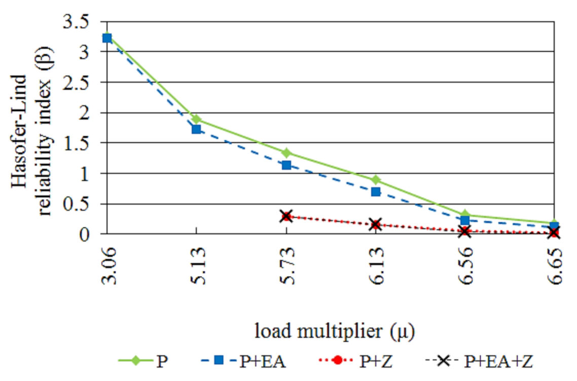
The analysis shows how the introduction of random variables affects the value of the Hasofer–Lind reliability index (Figure 7). Values of the dimensionless load multiplier, µ, in Figure 7 are selected points on equilibrium path in Figure 6, near coordinates of limit point.

Based on Figure 7, we can conclude that the highest values of the reliability index are obtained when the random variable is only the load, P. The addition of further variables (axial stiffness, EA, and coordinate of the first node, Z) significantly reduces the value of the reliability index. In addition, we can see that a much larger impact on the probability value of failure has a random variable Z than EA variable. For example, for the value of load multiplier μ = 5.73 and description of the mathematical model by variables P and EA, the reliability index assumes the value of β = 1.135, while the introduction of another variable Z reduces the value of the indicator by 74% (β = 0.29). This confirms the thesis argued in the literature that imperfections of node positions play a very important role in structures susceptible to node snapping in probabilistic and deterministic analysis.

4.3. FNE Method

4.3.1. Computation of Patterns

In the presented FNE method, the loads parameter μ for few equilibrium points of the structure corresponding to i-th randomly selected sample X_i is computed by means of NN mapping:

$${\mathbf{X}}_{N\times 1}=\left\{x_1,x_2,\dots ,x_n\right\}\stackrel{\hspace{1em}\mathrm{NN}\hspace{1em}}{\to }y=\mu ,$$

(9)

where: $x_i$—random variable corresponding to geometric values or material characteristics of the analyzed structure, y—NN output.

According to the block diagram shown in Figure 1, the training and testing patterns were computed by FEM. The authoring program, implemented in MATLAB environment, was applied.

The training patterns were computed for the input data placed regularly in the 3D-cube of coordinates P∈[−3σ_P, 3σ_P], EA∈[−3σ_EA, 3σ_EA], Z∈[−3σ_Z, 3σ_Z], assuming 4 points on the P, EA, Z axes, the number of training patterns equals L = 3⁴ = 64, cf. [25]. The set of T = 80 testing patterns was randomly selected as 80 points in the 3D-cube of variables P, EA, Z, assuming normal probability density function with the same parameters as for the training patterns. Description of input data and their random parameters is shown in Table 1.

In Figure 8 the equilibrium path μ_FEM(q) computed for the mean value of random variable (Table 1) is shown.

The procedure of deriving the explicit formulas defining the location of points on the equilibrium path was shown on an example of the point marked with the number 1 (see Figure 8).

4.3.2. Design of NN

At the second stage of FNE method to formulate explicit state functions at every marked equilibrium point (Figure 8) a feed-forward Multilayer Perceptron (MLP) with back-propagation of errors was used. MLP is the classic, most commonly used network structure in engineering issues. The neural network using the Neural Network Toolbox was designed [37]. It was formed by neurons arranged in layers with one direction of signal flow. In the later numerical analysis, the MLP with one hidden layer: X–H–Y, where X as the number of inputs, H as the number of neurons in hidden layer, and Y as the number of outputs were applied. After initial computations, for further analysis the group of networks with the MLP:3–H–1 architecture was accepted. The inputs to the networks were three parameters assumed in the task X = {P, EA, Z} as random variables (

Table 2. Features of task parameters.

Parameter	Range of Values		Scaling Factor	After Scaling
	Min	Max		Min	Max
P (kN)	8	12	SP = 12.6	0.6375	0.9524
EA (kN)	347004	518364	SEA = 544280	0.6375	0.9524
Z (m)	−0.1	0.1	SZ = 0.105	−0.9524	0.9524
μ	dependent on the equilibrium point		Sμdependent on the equilibrium point	dependent on the equilibrium point

). The single output was the load multiplier, Y = {μ}, in each of the 1–6 points of the equilibrium path.

When using a MLP neural network equipped with sigmoidal activation functions, it is necessary to perform scaling or normalization of data provided as the network inputs and outputs. Lack of proper transformation causes serious disruptions in the learning process and inferior properties of the learned network. The expected output values should not take the upper or lower limit of the activation function. This range should not exceed [0; 1] and [−1; 1], respectively, for a sigmoid and a symmetrical (bipolar) sigmoid function of activation. For inputs data, there are no such strict limits; they can be scaled to the same values as the outputs. It is important that they are close to zero and have a small amplitude. Scaling is absolutely necessary when the data represent a different order of magnitude (see Table 2).

The following simple formulae of scaling are proposed in this paper:

$$S_{f,x}=\frac{\max \left|x\right|}{1.05},$$

(10)

where S_f,x is the scaling factor of real value x, and x is the vector of real value x. When determining the scale factor, the denominator was 1.05. This value was determined on the basis of our own numerical tests. The network usually achieves the best results when the denominator is in the range of 1.01 ÷ 1.10. Such a value causes that the scaled da-ta does not exceed the range [−1, 1], i.e., the asymptotes limiting the bipolar sigmoid activation function.

All the neural networks were trained by using the Levenberg–Marquardt (LM) learning algorithm. The LM method is an implementation of Newton’s optimization strategy [38]. It is characterized by fast convergence, relatively easy calculations, and transparent implementation. The bipolar sigmoid activation function (tanh(x)) in the hidden layers and the linear activation function in the output layer were assumed.

The learning process of the network has been verified by mean-square-error, MSE(V); standard error, stε(V); and relative errors ep_i, ep, and epV_avr:

$$MSE(V)=\frac{1}{V\cdot M}{\displaystyle \sum _{p=1}^V{\displaystyle \sum _{p=1}^M{\left(z_i^{(p)}-y_i^{(p)}\right)}^2}},$$

(11)

$$st\epsilon (V)=\sqrt{\frac{1}{V\cdot M}{\displaystyle \sum _{p=1}^V{\displaystyle \sum _{p=1}^M{\left(z_i^{(p)}-y_i^{(p)}\right)}^2}}},$$

(12)

$$e{p}_i=\left(1-\raisebox{1ex}{$z_i^{(p)}$}\!\left/ \!\raisebox{-1ex}{$y_i^{(p)}$}\right.\right)\cdot 100\%,\left|e{p}_i\right|=\left|1-\raisebox{1ex}{$z_i^{(p)}$}\!\left/ \!\raisebox{-1ex}{$y_i^{(p)}$}\right.\right|\cdot 100\%,ep=\frac{1}{M}{\displaystyle \sum _{i=1}^M\left|e{p}_i\right|},$$

(13)

$$e{V}_{\mathrm{avr}}=\frac{1}{V\cdot M}{\displaystyle \sum _{p=1}^V{\displaystyle \sum _{i=1}^M\left|e{p}_i\right|}},$$

(14)

where $z_i^{(p)}$ and $y_i^{(p)}$ are the target and neurally computed i-th outputs for p-th pattern; M is the number of outputs; and V = L,T,P—number of learning (L), testing (T), and all (P) patterns, respectively. In

Table 3. Errors of Multilayer Perceptrons (MLPs):3 –H–1 formulated in the limit point.

Number of Hidden Neurons H	ep (%)		max epi (%)
	L	T	L	T
2	7.34	8.06	48.45	64.21
3	1.01	1.80	4.22	10.79
4	0.93	1.09	4.09	7.10
5	0.30	0.37	2.43	3.93
10	0.07	0.11	0.55	1.74
15	0.01	0.14	0.54	4.17
20	0.09	0.27	0.69	10.04
25	0.11	0.99	0.86	36.50
30	0.08	1.55	1.65	56.61

, the calculated values of selected errors for prepared networks’ architectures are presented.

The successive phases in signal processing in the MPL network are not so-called “black box”. They can be described as a relatively simple mathematical expression. However, for most tasks, there is no such need [39]. When developing any approximating formula, the simplest form is usually aimed at. This allows for the easier use of the equation in various computing environments. When the formula is derived from the structure and parameters of the neural network, the following principle should be followed: small network → simple approximation formula. At the same time, all rules regarding the correctness of building NN for a given task should be kept.

Figure 9 shows a graph of the percentage error—average (a) and maximum (b) depending on the number of neurons in the hidden layer. The optimal number of hidden neurons, H = 5, was picked out by using the cross-validation procedure (see Reference [40]).

Moreover, the linear regression coefficient, r(V), was computed for every set of pairs.

Figure 10 shows the correlation of load multipliers calculated by using FEM and NN. This correlation is close to unity for both the teaching and testing patterns.

The output from the network, that is dependence ${\mu }_{NN}$(P, EA, Z) (15), can be formulated explicitly, through the known values of the network parameters:

$${\mu }_{NN}(P,EA,Z)=S_{\mu }\cdot (w_{YH}\cdot (\tanh (w_{HX}\cdot \left[\begin{array}{ccc}\frac{P}{S_P}& \frac{EA}{S_{EA}}& \frac{Z}{S_Z}\end{array}\right]{}^T+b_H))+b_Y,$$

(15)

where $w_{HX}$ is the weight of input (X) and hidden (H) layers connections; $w_{YH}$ is the weight of output (Y) and H layers connections; $b_H$ and $b_Y$ are the biases of neurons of subsequent layers of the network. Network parameters (weight and biases) are most often calculated iteratively in the learning process.

After a decomposition, the formula on ${\mu }_{NN}$ (15) for the vertical displacement of the truss top node, which is w₁ = 7.20 cm, can be represented, for example, as follows (16):

$$\begin{array}{ll}{\mu }_{NN}(P,EA,Z)& =14.68\cdot \tanh (6.9102\cdot {10}^{-2}\cdot P-1.9365\cdot {10}^{-6}\cdot EA-3.1885\cdot Z+0.94164)\\ & -10.481\cdot \tanh (1.9158\cdot {10}^{-1}\cdot P-3.2239\cdot {10}^{-6}\cdot EA+2.7838\cdot Z+0.86115)\\ & -4.179\cdot \tanh (-6.6649\cdot {10}^{-2}\cdot P+1.3313\cdot {10}^{-6}\cdot EA+135.8\cdot Z-6.3707)\\ & +4.4871\cdot \tanh (-9.8057\cdot {10}^{-2}\cdot P+3.7886\cdot {10}^{-6}\cdot EA-2.2308\cdot Z-0.5907)\\ & +6.0319\cdot \tanh (-8.2171\cdot {10}^{-2}\cdot P+1.5887\cdot {10}^{-6}\cdot EA+15.168\cdot Z-0.43125)\\ & +4.8655.\end{array}$$

(16)

The above procedure was applied to formulate explicit state functions at every equilibrium point. The MLP:3-5-1 structure of the network was selected as the optimal approximator in this example. Relative percentages errors for learning and testing did not exceed 1% (

Table 4. Maximum relative percentages errors for learning and testing and linear regression coefficient computed for every marked point of equilibrium path.

Equilibrium Point (w) [cm]	${\mathit{\mu }}_{\mathit{F}\mathit{E}\mathit{M}}$	${\mathit{\mu }}_{\mathit{N}\mathit{N}}$	ep (%)		r(T)
	Computed for Mean Value of Random Variable		L	T
1 (7.20)	6.65	6.6636	0.30	0.37	0.999
2 (6.19)	6.56	6.5656	0.35	0.39	0.999
3 (5.07)	6.13	6.1417	0.83	0.94	0.998
4 (4.46)	5.73	5.7586	0.42	0.46	0.999
5 (3.74)	5.13	5.1203	0.20	0.22	≈1.00
6 (1.95)	3.03	3.0586	0.49	0.56	0.999

).

4.3.3. Results—FNE Method

The next stage of the FNE method, after preparing the approximation formulas (15) for the points marked on the balance path (Figure 8 and Table 4), is the reliability analysis and determination of the reliability index β. In this case, NUMPRESS software was also used [35]. The previously mentioned FORM was selected for analysis. In the formula for limit state function (8), parameter µ(X) was the function of random variables describing by explicit state functions (15, 16). Load multiplier ${\mu }_{NN}$(X) was directly computed by the reliability program. The analysis shows how the introduction of random variables affects the value of the Hasofer–Lind reliability index (Figure 11). Values of dimensionless load multiplier, µ, in Figure 7 are selected points on equilibrium path in Figure 6.

The tendency in the reliability index results is the same as in the case of the FE method. The highest values of the reliability index are obtained when the random variable is only the load, P (Figure 11). The use of mathematical models with imperfections of node positions results in the reduction of the reliability index value.

5. Comparison and Discussion of Results

The main objective of this article about performed studies was to demonstrate that hybrid systems combining neural networks and conventional computations are suitable for explicit formulation of limit state functions. For this purpose, the training dataset computed by FEM was needed. A well-chosen number of elements in the training set caused the trained network to have good generalization of properties in spite of simple architecture. The biggest error in testing formula did not exceed 1%. These properties indicate good efficiency of the resulting proposed approach. This approach is applicable to structural reliability problems with a wide arrange of variations, including the number of random variables, the random variable distributions, and the performance function.

The second issue was the reliability of the structure, depending on the adopted number of random variables. Our considerations concern Figure 7 and Figure 11. This figures show changes in reliability index values while following the non-linear geometric solution path, when load P is the only random variable (Series 1). The remaining parameters of the problem are treated as deterministic variables. The values of the reliability index obtained with such a computational model are clearly higher than those in other series, which provides a much more comprehensive description of the problem (random variables describe the following: load P, bar axial stiffness EA, and coordinate Z of node 1). We observed that the lowest values of reliability index are for case where we have the highest number of variables (P + EA + Z). In addition, we can see that a much larger impact on the probability value of failure has a random variable Z than EA variable. Accounting for a larger number of random variables extends the computation time, yet such a manner of formulating the problem makes it possible to give a more accurate evaluation of a structure safety.

A comparison of the FI method and FNE method is shown in

Table 5. Comparison of calculation method for mathematical model description describing with random variable P.

μ(X) Values	Values of Hasofer–Lind Reliability Index		ep (%)
	βFI	βFNE
3.06	3.264	7.361	125.5
5.13	1.891	2.328	23.1
5.73	1.34	1.423	6.2
6.13	0.892	0.846	5.2
6.56	0.32	0.343	7.2
6.65	0.177	0.171	3.4

,

Table 6. Comparison of calculation method for mathematical model description describing with random variable P+EA.

μ(X) Values	Values of Hasofer–Lind Reliability Index		ep (%)
	βFI	βFNE
3.06	3.218	5.785	79.8
5.13	1.722	1.835	6.6
5.73	1.135	1.073	5.5
6.13	0.699	0.624	10.7
6.56	0.225	0.204	4.9
6.65	0.121	0.107	11.6

,

Table 7. Comparison of calculation method for mathematical model description describing with random variable P+Z.

μ(X) Values	Values of Hasofer–Lind Reliability Index		ep (%)
	βFI	βFNE
3.06	-	-
5.13	-	-
5.73	0.293	1.002	242.0
6.13	0.161	0.171	6.2
6.56	0.047	0.045	4.3
6.65	0.024	0.025	4.2

and

Table 8. Comparison of calculation method for mathematical model description describing with random variable P+EA+Z.

μ(X) Values	Values of Hasofer–Lind Reliability Index		ep (%)
	βFI	βFNE
3.06	-	-
5.13	-	-
5.73	0.29	0.772	166.2
6.13	0.158	0.167	5.7
6.56	0.047	0.043	8.5
6.65	0.024	0.022	8.3

. The relative percent error (13) for each description of the mathematical model does not exceed 12% beyond the points furthest from coordinates of the limit point (for µ = 3.06). The results obtained refer to the value of the load multiplier near the limit point. During the analysis for lower values, there were problems with calculating the gradient limit functions necessary to determine the position of the design point. It is the reason of high values of relative percent error for µ = 3.06.

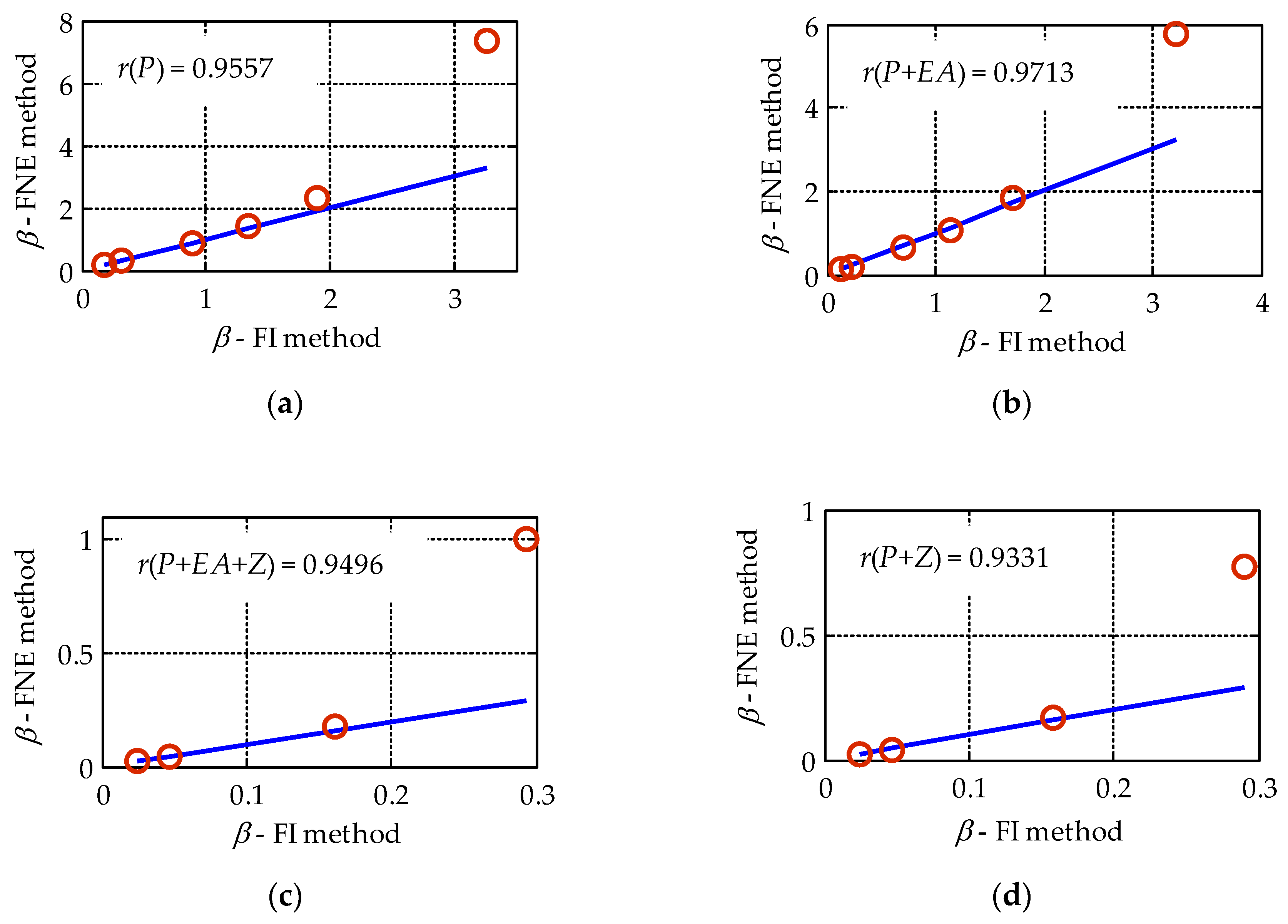
On the basis of Hasofer–Lind reliability values (β_FI, β_FNE) for four mathematical model descriptions, the linear regression coefficient r(V) was computed (Figure 12). The points placed on the diagonal correspond to the perfect overlapping of results. The correlation coefficients for all adopted mathematical models of reliability analysis are not less than 0.93. In each case, there is only one pair of compared results (β_FI–β_FNE) which significantly disturb the correlation.

The search for an effective and accurate method of reliability analysis for real constructions takes up a lot of space in the contemporary literature. The FI method is a known and often-used method, whereas the hybrid FNE method is an alternative method that is based on the use of neural networks. In the opinion of the authors, in the future, it would be tempting to compare the results of the reliability index with other methods of reliability analysis. This would allow a more accurate assessment of which method can be considered reliable despite some approximations. In this paper, the FI method was the reference method. The FNE method can be treated as a method with a double approximation error. The first error is obtained from the finite element method. In a task concerning non-linear construction work, the numerical solution will never coincide with the actual results. The second approximation error is generated during the formulation of the neural network. The percent error of matching formulas to the results obtained from FEM for the selected group of neural networks (MLP:3-5-1) did not exceed 1% (Table 4). This proves a very good fit of Formulas (15,16) to the results obtained from the original FEM program.

During reliability analysis using the traditional reliability prediction methods of more complicated types of structures, the explicit forms of limit state functions may lose their functionality [15]. The proposed hybrid approach is a convenient alternative in such cases, especially when it is necessary to calculate the sensitivity of the reliability index due to some random parameters of the task.

Reference [22] presents the reliability analysis by using implicit performance functions generated by NN and the comparison of the results of the reliability index with other methods. Meanwhile, Reference [23] presents an explicit formulation of the limit state function. This article should be treated as a progression and extension of the method presented in the mentioned publications.

6. Conclusions

Using the various methods of reliability analysis, moving along the equilibrium path of structure, we can determine reliability index and hence the level of failure probability when we approach the limit point.

It should be emphasized that, in engineering practice, it is very difficult to use an implicit form of limit state function because the calculation time increases with the number of random variables and the complexity of the structure. This problem partially was solved by employing explicit limit state functions developed by using a hybrid computational system with neural networks (FNE method). The article provides a ready-to-use procedure for the determination of explicit state functions by means of NN. The numerical costs of developing explicit limit state functions were relatively low in subjective evaluation. To prepare data, any FEM program can be used without the need to integrate it with a reliability program. The final stage of determining the reliability index was also carried out in the NUMPRESS program.

The first method (FI method) is well-known and is often presented. It was used to verify the results obtained with the proposed hybrid approach.

Based on performed analysis, it can be concluded that the results from both methods are similar, so they can be applied interchangeably, depending on the complexity of the analyzed structure. The results of structures analysis with the use of neural networks, known from the literature, confirm the advisability of using new approaches for civil-engineering problems, including the hybrid approach used in the work.