Article

Region Pixel Voting Network (RPVNet) for 6D Pose Estimation from Monocular Image

College of Electronic and Information Engineering, Tongji University, 4800 Cao’an Highway, Shanghai 201804, China
*
Authors to whom correspondence should be addressed.
Appl. Sci. 2021, 11(2), 743; https://doi.org/10.3390/app11020743
Submission received: 1 November 2020 / Revised: 9 January 2021 / Accepted: 12 January 2021 / Published: 14 January 2021
(This article belongs to the Section Robotics and Automation)

Abstract

:
Recent studies have shown that deep learning achieves superior results in the task of estimating 6D-pose of target object from an image. End-to-end techniques use deep networks to predict pose directly from image, avoiding the limitations of handcraft features, but rely on training dataset to deal with occlusion. Two-stage algorithms alleviate this problem by finding keypoints in the image and then solving the Perspective-n-Point (PnP) problem to avoid directly fitting the transformation from image space to 6D-pose space. This paper proposes a novel two-stage method using only local features for pixel voting, called Region Pixel Voting Network (RPVNet). Front-end network detects target object and predicts its direction maps, from which the keypoints are recovered by pixel voting using Random Sample Consensus (RANSAC). The backbone, object detection network and mask prediction network of RPVNet are designed based on Mask R-CNN. Direction map is a vector field with the direction of each point pointing to its source keypoint. It is shown that predicting an object’s keypoints is related to its own pixels and independent of other pixels, which means the influence of occlusion decreases in the object’s region. Based on this phenomenon, in RPVNet, local features instead of the whole features, i.e., the output of the backbone, are used by a well-designed Convolutional Neural Networks (CNN) to compute direction maps. The local features are extracted from the whole features through RoIAlign, based on the region provided by detection network. Experiments on LINEMOD dataset show that RPVNet’s average accuracy (86.1%) is almost equal to state-of-the-art (86.4%) when no occlusion occurs. Meanwhile, results on Occlusion LINEMOD dataset show that RPVNet outperforms state-of-the-art (43.7% vs. 40.8%) and is more accurate for small object in occluded scenes.

1. Introduction

Estimating the accurate 6D-Pose of certain objects has important implications in industries such as e-commerce and logistics [1], as pose information helps robotic systems to better manipulate materials. Monocular camera is one of the most common used sensors in pose estimation, due to its low cost, rich information and easy installation. However, since the 3D coordinates of spatial points cannot be obtained directly by a monocular camera, estimating the 6D-pose of an object from an image is a great challenge in research.
If the prior 3D model of target object is given, the Perspective-n-Point (PnP)-like algorithms [2] can theoretically solve the problem. The correspondence between the points on the model and the points on the picture is firstly determined. These corresponding points are constrained by the rigid transformation from model to camera. Thus, the object’s pose in the camera coordinate can be calculated. Traditional methods use handcraft features [3,4,5,6] to detect the model’s corresponding keypoints in the image. However, handcrafted features are not robust to changes in the environment. Template matching is also a common idea. Typical methods [7] extract prior templates from images of objects taken in various poses and estimates the poses of objects in image by matching these templates. Similar to handcraft-features, such templates are sensitive to environmental change.
With the development of deep learning, researchers try to dig the 6D-Pose information from 2D image in a machine learning way. In terms of network structure and function, machine learning methods can be roughly divided into two categories: end-to-end method and two-stage method.
End-to-end methods try to predict the pose of target object directly from the input image. For example, PoseNet [8] uses Convolutional Neural Networks (CNN) to regress the 6D pose of camera directly. Since detection is a prerequisite for pose estimation, i.e., an object’s pose cannot be predicted even before it is detected in the image, some studies have utilized results from the field of object detection. Based on Mask R-CNN [9], Deep-6DPose [10] adds a CNN branch as pose regression head to predict pose. However, directly predicting object’s position is difficult due to the large searching space and lack of depth information. By predicting the depth of the object center, PoseCNN [11] recovers the object’s pose with its 2D localization in image. Some studies transform pose regression into classification problem. For example, SSD-6D [12], which is built up the SSD [13], uniformly discretizes the object’s pose space with different viewpoints on a fixed radius. After the most probable rotation is classified, the translation is obtained by projection relations, and the final pose is obtained by refinement. A similar strategy of discretizing the pose space and predicting rotation by classification was adopted by Su et al. [14] and Sundermeyer et al. [15]. Such discretization leads to coarse pose predictions and often requires additional refinement to obtain accurate pose. The prediction accuracy of end-to-end method in occluded scenes decreases, and in practice it generally requires mixing in occluded samples for training to improve.
Two-stage methods generally predict the object’s keypoints on the image and then estimate the object’s pose with PnP algorithm. The method proposed in [16,17] designs a YOLO-like [18] architecture to predict the locations of the projected vertices of the object’s 3D bounding box. A similar approach was adopted by BB8 [19], which first finds the object’s 2D center and then regresses the projection of the eight vertices of its 3D bounding boxes in the image with a CNN network. These methods do not accurately predict the keypoints in occluded scenes. The research on human keypoints detection is well developed [20,21], and many studies are inspired by them. After finding the center point of an object, Centernet [22] regresses to the heatmaps for projections of 3D bounding boxes. To find the object’s bounding box, Zhou et al. [23] used Faster R-CNN [24] and an hourglass architecture to predict the keypoints’ heatmaps. To obtain accurate and robust prediction for keypoints, Oberweger et al. [25] predicted heatmaps from multiple small patches independently and accumulated the results. However, predicting heatmap also has a disadvantage when dealing with occlusion cases, as the occluded keypoints may not produce significant values on the heatmap, which may lead to estimation error.
Another kind of two-stage methods produce intermediate values for every pixel or patch and then determine the final result in a manner similar to a Hough voting [26]. For example, Michel et al. [27] used conditional random field to generate the small number of pose hypotheses which will be selected through voting. In the study by Branchman et al. [28], the proposed method regresses coordinates and object labels using automatic context and random forest, makes an initial pose estimation through fixed Random Sample Consensus (RANSAC) hypotheses and finally refines the estimation using the uncertainty of coordinates. However, regressing coordinates is hard due to large output space. Thus, PVNet [29], which is the state-of-the-art, predicts vector pointing to a keypoint in the image for every pixel that belongs to the object, and produce the keypoints via a voting procedure, and then a PnP procedure is adopted for final pose estimation. PVNet uses the whole features for prediction. The disadvantage of whole features is that most of them are not relevant to the object to be estimated, considering that the target object generally occupies a very small part of the picture.
To estimate the 6D-pose from image with high accuracy in occluded scenarios, a novel two-stage algorithm called RPVNet is proposed. The backbone, object detection network (detection head) and mask prediction network (mask head) are designed based on Mask R-CNN, ResNet18 [30], and Feature Pyramid Network (FPN) [31] is used to construct the backbone; the detection head is built by a simple fully connected network. After inputting the original image, backbone produces features of different scales. With the regions provided by Region Proposal Network (RPN), detection head uses these features to produce the object’s bounding box. We point out that predicting an object’s keypoints is related to its own pixels and independent of other pixels. Thus, as a main contribution, we use local features instead of the whole features to compute the direction maps. Direction map is a vector field with the direction of each point pointing to its source keypoint. With the region specified by the bounding box, local features are extracted from the whole features through Region of Interest (RoI) Align. Keypoint detection head, which is implemented by a well-designed CNN, uses the local features to generate direction maps. After the direction maps are aligned with original image, the keypoints are recovered by pixel voting using RANSAC. Finally, given the keypoints’ prior 3D coordinates, the 6D-pose can be calculated by solving the PnP problem.

2. Materials and Methods

2.1. Model of the Problem

In this section, a mathematical model of the problem is presented. The concept of pose in this article is first defined. Then, the equivalence between object’s pose estimation and camera’s external parameter estimation is revealed. Finally, it is shown that the goal can be achieved in a PnP way, as long as the keypoints of target object are correctly found in the image.

2.1.1. Pose of an Object

The pose of an object refers to its spatial position and attitude angle. A fixed coordinate system, commonly called the world coordinate system (WCS), is required to describe pose. If a three-dimensional Cartesian coordinate system called object coordinate system (OCS) is artificially fixed on the object, then the object’s pose is defined as follows:
Definition 1.
If WCS coincides with OCS after applying a virtual rotation R and translation t , then [ R w o | t w o ] is called the pose of the object’s in WCS.
The superscript of R and t represents the target coordinate system and the subscript represent the source coordinate system.
However, in practice, the pose of an object is not calculated according to Definition 1 because it is not possible to actually fix a coordinate system on the object. Instead, a Computer Aided Design (CAD) or point cloud [32] model of the same size as the object is virtually fixed at the origin of another virtual coordinate called M o d e l . Then, the object’s pose in M o d e l is defined as:
Definition 2.
For any point P on the object, its coordinates in M o d e l is P o m o d e l , if P m is its corresponding point on the model in M o d e l , and satisfy P o m o d e l = R m o · P m + T m o , then R m o T m o is the object’s pose in M o d e l .
Note that P o represents the coordinates of P in OCS, and P o m o d e l represents the coordinates of P in M o d e l . Since the model is exactly equal to the object, P o is equal to P m .

2.1.2. Equivalence between Pose and Camera External Parameter

Let us first review the pinhole model for monocular camera. Considering a point P, its coordinates in WCS and CCS (camera coordinate system) are P w and P c , respectively. Then,
P c = R c w · P w + T c w
If ( x p , y p ) is the coordinate of the projection point of P on the picture under the image coordinate system (ICS), given the intrinsic parameter K, ( x p , y p ) can be expressed as:
x p y p 0 = 1 z c K · P c , where   z c   is   z   coordinate   of   P c   and   K = f x 0 c x 0 f y c y 0 0 1
[ R c w | T c w ] is known as the external parameter.
According to Definition 2, if the monocular camera coordinate system CCS coincides with M o d e l and the WCS coincides with the OCS, then the object’s pose [ R m o | T m o ] in M o d e l is equivalent to the camera external parameter [ R c w | T c w ] . Thus, the following corollary can be drawn:
Corollary 1.
Given the object’s model and the camera’s external parameter [ R c w | T c w ] , then, for point P on the object, the coordinate of its projection in the image is:
x p y p 1 = 1 z c K · ( R c w · P m + T c w )

2.1.3. PnP Based Pose Estimation

Corollary 1 states that, for a given camera (the intrinsic K is fixed), the object’s projection on the image can be inferred, given the prior model of the object and the camera’s external parameter. Considering the equivalence of the camera’s external parameter and the object’s pose, it is the inverse that needs to be concerned in pose estimation: given the picture of the object, the camera’s intrinsic parameter and the object’s prior model, find the camera’s external parameter.
Noting that P m equals P o and that OCS coincides with WCS, this problem becomes a typical PnP problem. There have been many well-developed solutions on how to solve PnP: Direct Linear Transform (DLT) [33], Perspective-3-Point (P3P) [34], Efficient PnP (EPnP) [2], etc. Thus, the key to solving the pose estimation is to find exactly where the keypoints of the object are projected in the image.

2.2. Proposed Method

According to Section 2.1.2, if the corresponding 2D projections of object’s keypoints can be found in the image, then the pose can be inferred through PnP algorithm. Traditional methods extract handcrafted features to detect keypoints in the image. However, they are not robust to complex environment.
Deep learning methods have been proven to be effective in keypoints prediction. The proposed method takes a two-stage pipeline: the front-end network uses local features to predict direction maps, from which the keypoints are recovered through RANSAC voting. Then, the pose is computed through PnP algorithm.

2.2.1. Network Structure

The overall structure of the two-stage pipeline is shown in Figure 1.
Backbone consists of a ResNet18 [30] and a FPN [31]. ResNet performs convolution and pooling operations on the original image in four stages, using residual network [30]. FPN uses the strategy of upsampling to fuse the results from different stages and outputs features at different scales. A feature is a C × H × W tensor, where C, H and W are channel number, height and width, respectively, and its scale is controlled by H and W. RPN takes these feature as input and produces region proposals based on some pre-generated anchors. With RoIs and the features from backbone, detection head provides accurate bounding boxes with objects’ classes information [9].
Instead of using the whole features for keypoints detection as in PVNet [29], the regions specified by the predicted bounding boxes are utilized to select local features by RoIAlign [9]. The keypoint head consists eight convolutional layers and one deconvolutional layer. Its structure is determined experimentally. The keypoint head generates raw direction maps with the local features. The final direction maps can be obtained by masking the raw direction maps with the prediction from mask head, which is designed based on Mask R-CNN [9].
After aligning the direction maps with the origin image, keypoints in the image are recovered by pixel voting through RANSAC. With the predicted keypoints and the corresponding keypoints on the priori point cloud model [32], the 6D-Pose is calculated by solving PnP. In this study, EPnP [2] is selected as the PnP algorithm.

2.2.2. Keypoints Selection

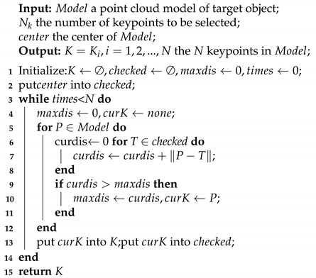
Keypoints can be selected manually, but it lacks scalability. The farthest sampling strategy is adopted to select keypoints on the prior point cloud model: the center of the point cloud is initially selected; then, the farthest point from selected keypoints is repeatedly chosen from the point cloud. The detail of farthest sampling is shown in Algorithm 1. As suggested by PVNet [29], N k is set to 8 in our model.
Algorithm 1: Farthest Sampling
Applsci 11 00743 i001
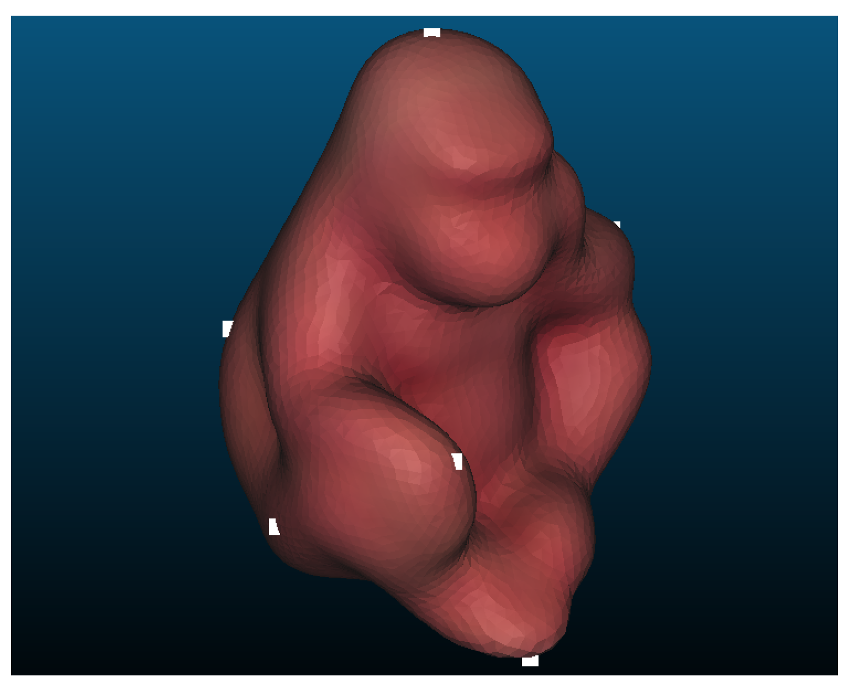
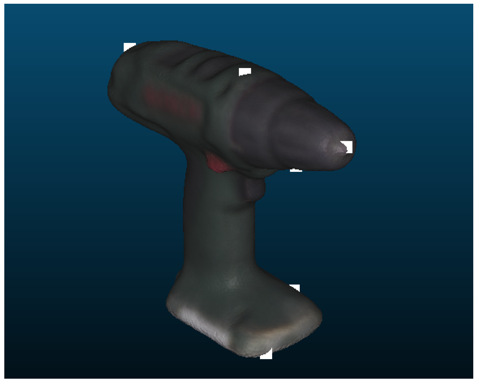
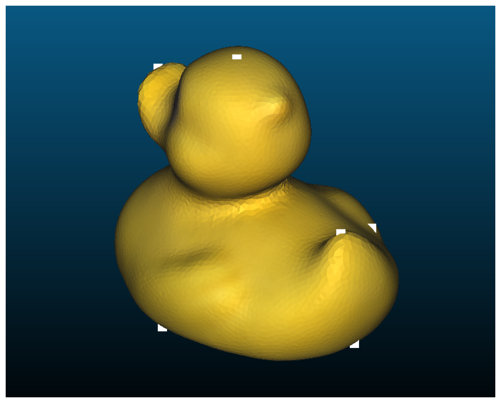
In Figure 2, Figure 3, Figure 4 and Figure 5, the white dots show the selected keypoints of several types of objects in LINEMOD [35]. LINEMOD is a standard dataset; more details can be found in Section 3.1.

2.2.3. Direction Map

Predicting keypoints with heatmap is widely used in fields such as human posture estimation [20,21]. In heatmap, the closer a point is to a keypoint, the greater the probability that it is a keypoint. Normal distribution is commonly used to describe this probability. However, this is not a good way to handle cases where keypoint is blocked, since part of heatmap is occluded as well. If the size of the Gaussian kernel is chosen too small, the entire heatmap will not have a significant value. As a countermeasure, the complete heatmap can still be predicted for the occluded keypoint, as if it was not blocked. However, this is actually predicting the keypoint’s heatmap with the obstacle’s pixels, which have nothing to do with the object. This affects the training performance and results in large prediction errors.
The proposed method adopts a strategy of direction map [29]. The direction map is defined as follows.
Definition 3.
For a given I m a g e , k I m a g e and is the target object’s keypoint in I m a g e . Then, the direction map of k in the image is:
D ( k ) = d p = ( p , d i r ) | p I m a g e , d i r = I n d i ( p o b j ) k p k p
where I n d i ( p o b j ) = 1 i f   t u r e N a N o t h e r w i s e
As introduced in Section 2.2.1, keypoint head consists of eight convolutions with stride 1 followed by one layer of deconvolution with stride 2. If the input feature is a tensor of size m d / 2 × n d / 2 , it outputs a m d × n d raw direction map.
According to Definition 3, it is clear that only pixels belonging to target object contribute to the direction map, which helps to shield the interference caused by the occlusion. Obviously, mask is needed to perform masking operations on raw direction map to get the final direction map. During inference, mask is provided by the mask head introduced in Section 2.2.1; during training, they are provided by ground truth mask.
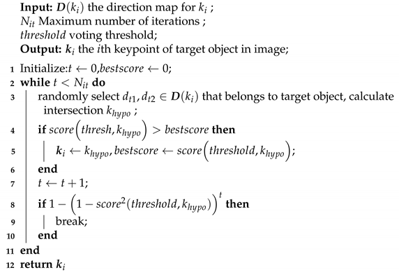
The 2D keypoints are inferred from the predicted direction maps through RANSAC voting, as shown in Algorithm 2. Note that Algorithm 2 is designed for only one keypoint, and all keypoints are predicted using the same algorithm.
Algorithm 2: RANSAC voting for a keypoint
Applsci 11 00743 i002
In our model, N i t is set to 512 and t h r e s h o l d is set to 0.99. The voting score is calculated as follows:
s c o r e ( t h r e s h h o l d , k ) = a v e r a g e d D I n d i k p k p · d i r > t h r e s h o l d

2.2.4. Using RoI for Detection

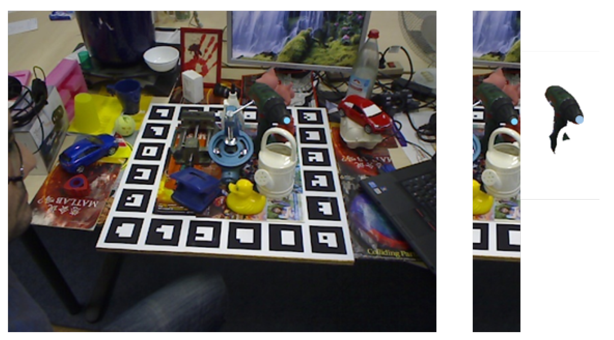
Keypoints and their direction maps are properties closely related to object they belong to. This means pixels that do not belong to the object are useless for prediction. As shown in Figure 6, the tip of the driller can still be predicted as the irrelevant pixels disappear.
Based on such a phenomenon, to predict direction maps, RPVNet uses RoIs to extract local features from the whole features by RoIAlign [9]. During inference, a proposed RoI is specified by the bounding box predicted by the detection head. During training, the RoIs generated by RPN are fed to keypoint head after non-maximum suppression [24], in which Intersection-over-Union (IoU) with ground truth bounding box above a certain threshold are selected for training.

2.2.5. Alignment of Direction Map

When using RoI, the direction map is predicted based on pixels inside it. Since the position and size of RoI may not be integer, RoIAlign [9] is adopted to extract fixed size features. Due to CNN structure, the size of direction map is fixed as well. It is necessary to align the direction map with its corresponding RoI and the image.
Assuming the direction map has m d rows and n d columns, the RoI is evenly divided into m d × n d patches and their centers are the corresponding position. If the height and width of the RoI is h and w, for the element at the ith row and jth column of direction map, its coordinates in the RoI is:
x r o i = w / n d ( i 0.5 ) , y r o i = h / m d ( j 0.5 )
Thus, the direction map can be aligned with the origin image. Assuming the left-up corner of RoI is ( x l u , y l u ) , then the elements position in the image is:
x = x l u + x r o i , y = y l u + y r o i

3. Results

3.1. Datasets

We used three datasets in our experiments.
LINEMOD [35] dataset is the most widely used standard dataset in the study of pose estimation. LINEMOD has collected ground truth data, including images, depth images and corresponding pose of each object, for 13 objects.
Meanwhile, it contains point cloud model for every kind of object. There are many challenging factors in LINEMOD, such as textless objects, cluttered scenes, etc. However, the target objects labeled in each image are not obscured. LINEMOD has an average of 1200 images per type of object, but only 150 images of each type are selected for training.
Occlusion LINEMOD [36] dataset uses the same objects in the similar scenes as LINEMOD, but the objects in the dataset are very heavily occluded from each other. This brings a particular challenge to pose estimation.
Truncation LINEMOD [29] dataset is created by randomly cropping each image of LINEMOD. Only 40–60% of the area of the target object is visible after cropping. This results in a very high pixel deficiency of the target object. Although this phenomenon is not easy to occur in practice and this paper is aimed at improving the accuracy of pose estimation when occlusion happens, we still conducted experiments on Truncation LINEMOD as an additional exploration.
Occlusion LINEMOD and Truncation LINEMOD are not involved in training at all. They are only used for testing.

3.2. Evaluation Metrics

The two most common evaluation metrics in the field of pose estimation are 2D projection error and average 3D distance (ADD).
2D projection error metric is defined as follows. Given the object’s model and camera’s intrinsic parameters, the selected points on the model are projected onto the image according to the ground truth pose and estimated pose, respectively. If the average distance in image between corresponding 2D points is less than 5 pixels, then the estimated pose is considered as accurate.
For ADD metric, the object model, usually referred to as the point cloud model, is rigidly transformed according to the ground truth and estimated pose, respectively. If the average distance between the corresponding points of the two transformed models is less than 10% of the model’s diameter, then the estimated pose is considered to be accurate. The diameter of the model is defined as the distance between the two farthest points on the model. For symmetric objects, ADD-S metric [11] is used. In ADD-S, the average distance is calculated according to closest point distance.
In our experiment, only ADD metric was selected for accuracy evaluation. The main reasons are threefold: First, according to Equation (2), as the point’s depth z c increases, the change in pixels caused by the same relative motion of the object becomes smaller and smaller. Second, the experimental results of many studies [10,12,17,29] show that 2D projection error is more “tolerant” than ADD metric, i.e., accuracy is higher under the criterion of 2D projection error. Third, the purpose of estimating pose is often for other systems to better interact with the object in 3D space, which means that ADD metrics are more realistic.

3.3. Training Strategy

During training, smooth L1 function was selected as the loss function for the keypoint head. According to Section 2.2.3, the loss is:
L o s s k e y p o i n t = i = 1 N k P O L d i ( P | K i ) d i ¯ ( P | K i ) , where   L ( x ) = 1 2 α 2 x 2 if   | x | < α ( x 1 2 α ) otherwise
α is set to 0.25 in our model. Smooth L1 function and the softmax cross-entropy function were used as the the loss function for detection head and mask head, respectively.
To prevent overfitting, image augmentation and dataset expansion were used. Image augmentation, including rotation, scaling, cropping, color jittering, adding noise, etc., was randomly used during training. The strategy of cut and paste was adopted for dataset expansion: for training images, the target objects were extracted according to their masks and pasted onto random images. In total, 10,000 images were produced. In addition, virtual sampling and synthesis were also used. An object model was randomly pictured in the virtual environment and then pasted onto random image. For each type of object, 9000 images were generated in this way. The backgrounds of these composite images were all randomly sampled from ImageNet [37] as well as SUN397 [38].

3.4. Test Results

Testing experiments were conducted on the LINEMOD dataset, the Occlusion LINEMOD dataset and the Truncation LINEMOD dataset, using the ADD metric to evaluate accuracy (in %). Note that glue and eggbox are considered as symmetric objects, so their experimental results were evaluated by ADD-S.
The test results on LINEMOD is shown in Table 1. In “two-stage” part, the first column represents RPVNet and the second shows the results of the proposed method using heatmap instead of direction map. The remaining columns show the results of other studies, including end-to-end methods (Deep6D and SSD-6D) and two-stage methods (Tekin, BB8, Cull and PVNet).
The test results on Occlusion LINEMOD is shown in Table 2. In the table, PoseCNN is the only end-to-end method and others are two-stage method. The comparison between predicted and ground truth pose for RPVNet is shown in Figure 7: the 3D bounding box is projected onto the image according to the pose information. The green box represents predicted value, and the blue one represents ground truth.
The above two tables also show the average accuracy (Average) and the standard deviation (Std-Dev) for each method. In addition to this, the last row of each table, Wilcoxon t , shows the results (Yes/No) of the two-sided Wilcoxon rank sum test [39] at 0.05 significance level for the hypothesis “there is a significant difference between RPVNet and the method represented by the current column”.
The test result on Truncation LINEMOD is shown in Table 3. The last column, Wilcoxon t , shows the results of the two-sided Wilcoxon test for the hypothesis “there is a significant difference between RPVNet and the current method” at the significance level of 0.05.

4. Discussion

4.1. Comparison between Heatmap and Direction Map

The Wilcoxon test results show that there is a significant difference between RPVNet and the proposed method using heatmap on both LINEMOD and Occlusion LINEMOD. According to Table 1, on LINEMOD, the average accuracy of RPVNet (86.1%) is 5.3% higher than Heatmap method (81.7%). On Occlusion LINEMOD dataset, as shown in Table 2, the average accuracy of RPVNet, on the other hand, is about 47.6% higher than that of Heatmap method (43.7% vs. 29.6%). These results show that the use of direction map is more robust than heatmap in an occluded environment.
As explained in Section 2.2.3, the direction map remains relevant to the unobstructed part of the object, when occlusion happens. However, heatmap is located in a region of the image that is not part of the object, which means the network is predicting features that do not belong to the object. Thus, predicting the direction map is more robust than the heatmap.
A similar phenomenon was found in the study of PVNet [29], when comparing predicting keypoints on object, and predicting bounding-box corners. These results indicate that predicting the visible part of target object in the picture improves the robustness of keypoint predictions.

4.2. Comparison with Other Methods

Comparison with end-to-end methods. On LINEMOD, SSD-6D [12] with additional refinement and Deep6D [10] have average accuracies of 76.3% and 65.2%, respectively. On Occlusion LINEMOD, the accuracy of PoseCNN [11] is 24.9%. Although the standard deviation of RPVNet is not the best, the accuracy of RPVNet outperforms on both dataset (86.1%,43.7%,respectively) and the Wilcoxon tests verify this. Basically, end-to-end methods try to predict the pose of target objects directly from the features extracted from image, such as Deep6D and PoseCNN. Some might get more accurate result with refinement, such as SSD-6D. The pose of an object is a state space with six degrees of freedom. Its high dimensionality makes it difficult to directly predict pose from image, even if the range of values is restricted. In contrast, the object’s keypoints have only two degrees of freedom and are restricted to a specific area in the image, making the prediction easier and more accurate.
Comparison with two-stage methods. On LINEMOD, the average accuracy of RPVNet (86.1%) exceeds that of other two-stage methods except PVNet, such as Tekin (55.9%), BB8 (62.7%) and CullNet (78.3%). RPVNet (43.7%) is also more accurate than Tekin (6.4%) on Occlusion LINEMOD. The results of the Wilcoxon test verify that RPVNet is more accurate than these methods. If we compare PVNet with these methods, similar results can be drawn. This shows that estimating the keypoints on an object by predicting the direction map is more accurate than directly predicting the keypoints or the vertices of its bounding box.
PVNet is currently the state of the art. Although the average accuracy of RPVNet on LINEMOD (86.1%) is not higher than that of PVNet (86.4%), according to Table 1, RPVNet is considered close to PVNet, since the Wilcoxon test verifies that there is no significant difference between them. On Occlusion LINEMOD, RPVNet (43.7%) outperforms PVNet (40.8%), and the Wilcoxon test verifies this, which shows that there is significant difference between the two methods. RPVNet also performs better than PVNet When estimating small size objects in occluded scenes, such as ’ape’, ’cat’ and ’duck’. RPVNet uses the RoI specified by object’s bounding box to extract local features for prediction, while PVNet uses the whole features produced by backbone for prediction. These test results show that, in occluded scenes, using only partial features can improve robustness, as well as the accuracy of prediction for small-sized objects. Oberweger [25] also uses part of the features, but the performance (30.8%) is limited due to the drawback of heatmap and the random selection of local features.
Comparison on Truncation LINEMOD. According to Table 3, the average accuracy of RPVNet (31.3%) is close to that of PVNet (31.5%), which is supported by the Wilcoxon test. On the one hand, the images in the Truncation LINEMOD are relatively small, and the difference between whole features and local features is relatively small. On the other hand, the use of local features is also ineffective in reducing the interference of irrelevant pixels, when the pixels of the target object are extremely scarce.

4.3. Running Time

In addition, we also tested RPVNet’s running speed on a desktop computer. The test PC contained an Intel i7-9700K 3.6GHz CPU and a Nvidia RTX2070 GPU. Given an input of a 480 × 640 RGB image, the average processing speed was 42 ms, or 23 fps, which is close to PVNet (25 fps) [29].

5. Conclusions

To accurately estimate target object’s 6D-pose from a single image, a novel two-stage deep learning based method, RPVNet, is proposed. Instead of using the whole features from backbone, RPVNet uses local features to predict the object’s direction maps, which is our main contribution. After aligning the direction maps with original image, pixel voting is conducted through RANSAC to generate keypoints. Finally, the 6D-pose is recovered by solving PnP. In the experiment, RPVNet achieved 86.1% and 43.7% accuracy on LINEMOD and Occlusion LINEMOD, respectively. Compared with the state-of-the-art (86.4% and 40.8%, respectively), RPVNet has a estimation accuracy close to the top level and is more robust in the occluded scenes. In addition, RPVNet has higher accuracy when estimating small-sized objects in the occluded scenes. As part of future work, we plan to study pose estimation method for scenes with a severe lack of object pixels. The possibility of restoring object pixels using adversarial generation methods is being considered.

Author Contributions

Funding acquisition, C.L. and Q.C.; Methodology, F.X.; Project administration, Q.C.; Resources, Q.C.; Software, F.X.; Supervision, C.L. and Q.C.; Validation, F.X.; Visualization, F.X.; and Writing—original draft, F.X. All authors have read and agreed to the published version of the manuscript.

Funding

This research was funded by the National Natural Science Foundation of China (61673300, U1713211) and the Science and technology development fund of Pudong New Area (PKX2019-R18).

Conflicts of Interest

The authors declare no conflict of interest.

References

  1. Zeng, A.; Yu, K.; Song, S.; Suo, D.; Walker, E., Jr.; Rodriguez, A.; Xiao, J. Multi-view self-supervised deep learning for 6D pose estimation in the Amazon Picking Challenge. In Proceedings of the 2017 IEEE International Conference on Robotics and Automation, ICRA 2017, Singapore, 29 May–3 June 2017; IEEE: Piscataway, NJ, USA, 2017; pp. 1383–1386. [Google Scholar]
  2. Lepetit, V.; Moreno-Noguer, F.; Fua, P. EPNP: Accurate O(n) Solut. PnP Probl. Int. J. Comput. Vis. 2009, 81, 155–166. [Google Scholar] [CrossRef] [Green Version]
  3. Lowe, D.G. Object Recognition from Local Scale-Invariant Features. In Proceedings of the International Conference on Computer Vision, Kerkyra, Corfu, Greece, 20–25 September 1999; IEEE Computer Society: Washington, DC, USA, 1999; pp. 1150–1157. [Google Scholar]
  4. Lowe, D.G. Distinctive Image Features from Scale-Invariant Keypoints. Int. J. Comput. Vis. 2004, 60, 91–110. [Google Scholar] [CrossRef]
  5. Rublee, E.; Rabaud, V.; Konolige, K.; Bradski, G.R. ORB: An efficient alternative to SIFT or SURF. In Proceedings of the IEEE International Conference on Computer Vision, ICCV 2011, Barcelona, Spain, 6–13 November 2011; Metaxas, D.N., Quan, L., Sanfeliu, A., Gool, L.V., Eds.; IEEE Computer Society: Washington, DC, USA, 2011; pp. 2564–2571. [Google Scholar]
  6. Rothganger, F.; Lazebnik, S.; Schmid, C.; Ponce, J. 3D Object Modeling and Recognition Using Local Affine-Invariant Image Descriptors and Multi-View Spatial Constraints. Int. J. Comput. Vis. 2006, 66, 231–259. [Google Scholar] [CrossRef] [Green Version]
  7. Gu, C.; Ren, X. Discriminative Mixture-of-Templates for Viewpoint Classification. In Computer Vision—ECCV 2010, Proceedings of the 11th European Conference on Computer Vision, Heraklion, Crete, Greece, 5–11 September 2010; Daniilidis, K., Maragos, P., Paragios, N., Eds.; Lecture Notes in Computer Science; Proceedings, Part V; Springer: Berlin/Heidelberg, Germany, 2010; Volume 6315, pp. 408–421. [Google Scholar]
  8. Kendall, A.; Grimes, M.; Cipolla, R. PoseNet: A Convolutional Network for Real-Time 6-DOF Camera Relocalization. In Proceedings of the 2015 IEEE International Conference on Computer Vision, ICCV 2015, Santiago, Chile, 7–13 December 2015; IEEE Computer Society: Washington, DC, USA, 2015; pp. 2938–2946. [Google Scholar]
  9. He, K.; Gkioxari, G.; Dollár, P.; Girshick, R.B. Mask R-CNN. In Proceedings of the IEEE International Conference on Computer Vision, ICCV 2017, Venice, Italy, 22–29 October 2017; IEEE Computer Society: Washington, DC, USA, 2017; pp. 2980–2988. [Google Scholar]
  10. Do, T.T.; Cai, M.; Pham, T.; Reid, I. Deep-6dpose: Recovering 6d object pose from a single rgb image. arXiv 2018, arXiv:1802.10367. [Google Scholar]
  11. Xiang, Y.; Schmidt, T.; Narayanan, V.; Fox, D. PoseCNN: A Convolutional Neural Network for 6D Object Pose Estimation in Cluttered Scenes. In Proceedings of the Robotics: Science and Systems, Pittsburgh, PA, USA, 26–30 June 2018. [Google Scholar]
  12. Kehl, W.; Manhardt, F.; Tombari, F.; Ilic, S.; Navab, N. SSD-6D: Making RGB-Based 3D Detection and 6D Pose Estimation Great Again. In Proceedings of the IEEE International Conference on Computer Vision, ICCV 2017, Venice, Italy, 22–29 October 2017; IEEE Computer Society: Washington, DC, USA, 2017; pp. 1530–1538. [Google Scholar]
  13. Liu, W.; Anguelov, D.; Erhan, D.; Szegedy, C.; Reed, S.E.; Fu, C.; Berg, A.C. SSD: Single Shot MultiBox Detector. In Computer Vision—ECCV 2016, Proceedings of the 14th European Conference, Amsterdam, The Netherlands, 11–14 October 2016; Leibe, B., Matas, J., Sebe, N., Welling, M., Eds.; Lecture Notes in Computer Science; Proceedings, Part I; Springer: Berlin/Heidelberg, Germany, 2016; Volume 9905, pp. 21–37. [Google Scholar]
  14. Su, H.; Qi, C.R.; Li, Y.; Guibas, L.J. Render for CNN: Viewpoint Estimation in Images Using CNNs Trained with Rendered 3D Model Views. In Proceedings of the 2015 IEEE International Conference on Computer Vision, ICCV 2015, Santiago, Chile, 7–13 December 2015; IEEE Computer Society: Washington, DC, USA, 2015; pp. 2686–2694. [Google Scholar]
  15. Sundermeyer, M.; Marton, Z.; Durner, M.; Brucker, M.; Triebel, R. Implicit 3D Orientation Learning for 6D Object Detection from RGB Images. In Computer Vision—ECCV 2018, Proceedings of the 15th European Conference, Munich, Germany, 8–14 September 2018; Ferrari, V., Hebert, M., Sminchisescu, C., Weiss, Y., Eds.; Lecture Notes in Computer Science; Proceedings, Part VI; Springer: Berlin/Heidelberg, Germany, 2018; Volume 11210, pp. 712–729. [Google Scholar]
  16. Tekin, B.; Sinha, S.N.; Fua, P. Real-Time Seamless Single Shot 6D Object Pose Prediction. In Proceedings of the 2018 IEEE Conference on Computer Vision and Pattern Recognition, CVPR 2018, Salt Lake City, UT, USA, 18–22 June 2018; IEEE Computer Society: Washington, DC, USA, 2018; pp. 292–301. [Google Scholar]
  17. Gupta, K.; Petersson, L.; Hartley, R. CullNet: Calibrated and Pose Aware Confidence Scores for Object Pose Estimation. In Proceedings of the IEEE International Conference on Computer Vision Workshops, Seoul, Korea, 27 October–2 November 2019; pp. 2758–2766. [Google Scholar]
  18. Redmon, J.; Farhadi, A. YOLO9000: Better, Faster, Stronger. In Proceedings of the 2017 IEEE Conference on Computer Vision and Pattern Recognition, CVPR 2017, Honolulu, HI, USA, 21–26 July 2017; IEEE Computer Society: Washington, DC, USA, 2017; pp. 6517–6525. [Google Scholar]
  19. Rad, M.; Lepetit, V. BB8: A Scalable, Accurate, Robust to Partial Occlusion Method for Predicting the 3D Poses of Challenging Objects without Using Depth. In Proceedings of the IEEE International Conference on Computer Vision, ICCV 2017, Venice, Italy, 22–29 October 2017; IEEE Computer Society: Washington, DC, USA, 2017; pp. 3848–3856. [Google Scholar]
  20. Newell, A.; Yang, K.; Deng, J. Stacked Hourglass Networks for Human Pose Estimation. In Computer Vision—ECCV 2016, Proceedings of the 14th European Conference, Amsterdam, The Netherlands, 11–14 October 2016; Leibe, B., Matas, J., Sebe, N., Welling, M., Eds.; Lecture Notes in Computer Science; Proceedings, Part VIII; Springer: Berlin/Heidelberg, Germany, 2016; Volume 9912, pp. 483–499. [Google Scholar]
  21. Sun, K.; Xiao, B.; Liu, D.; Wang, J. Deep High-Resolution Representation Learning for Human Pose Estimation. In Proceedings of the IEEE/CVF Conference on Computer Vision and Pattern Recognition (CVPR), Long Beach, CA, USA, 15–20 June 2019. [Google Scholar]
  22. Zhou, X.; Wang, D.; Krähenbühl, P. Objects as Points. arXiv 2019, arXiv:1904.07850. [Google Scholar]
  23. Pavlakos, G.; Zhou, X.; Chan, A.; Derpanis, K.G.; Daniilidis, K. 6-DoF object pose from semantic keypoints. In Proceedings of the 2017 IEEE International Conference on Robotics and Automation, ICRA 2017, Singapore, 29 May–3 June 2017; IEEE: Piscataway, NJ, USA, 2017; pp. 2011–2018. [Google Scholar]
  24. Ren, S.; He, K.; Girshick, R.; Sun, J. Faster R-CNN: Towards Real-Time Object Detection with Region Proposal Networks. IEEE Trans. Pattern Anal. Mach. Intell. 2017, 39, 1137–1149. [Google Scholar] [CrossRef] [Green Version]
  25. Oberweger, M.; Rad, M.; Lepetit, V. Making Deep Heatmaps Robust to Partial Occlusions for 3D Object Pose Estimation. In Computer Vision—ECCV 2018, Proceedings of the 15th European Conference, Munich, Germany, 8–14 September 2018; Ferrari, V., Hebert, M., Sminchisescu, C., Weiss, Y., Eds.; Lecture Notes in Computer Science; Proceedings, Part XV; Springer: Berlin/Heidelberg, Germany, 2018; Volume 11219, pp. 125–141. [Google Scholar]
  26. Glasner, D.; Galun, M.; Alpert, S.; Basri, R.; Shakhnarovich, G. Viewpoint-aware object detection and pose estimation. In Proceedings of the IEEE International Conference on Computer Vision, ICCV 2011, Barcelona, Spain, 6–13 November 2011; Metaxas, D.N., Quan, L., Sanfeliu, A., Gool, L.V., Eds.; IEEE Computer Society: Washington, DC, USA, 2011; pp. 1275–1282. [Google Scholar]
  27. Michel, F.; Kirillov, A.; Brachmann, E.; Krull, A.; Gumhold, S.; Savchynskyy, B.; Rother, C. Global Hypothesis Generation for 6D Object Pose Estimation. In Proceedings of the 2017 IEEE Conference on Computer Vision and Pattern Recognition, CVPR 2017, Honolulu, HI, USA, 21–26 July 2017; IEEE Computer Society: Washington, DC, USA, 2017; pp. 115–124. [Google Scholar]
  28. Brachmann, E.; Michel, F.; Krull, A.; Yang, M.Y.; Gumhold, S.; Rother, C. Uncertainty-Driven 6D Pose Estimation of Objects and Scenes from a Single RGB Image. In Proceedings of the 2016 IEEE Conference on Computer Vision and Pattern Recognition, CVPR 2016, Las Vegas, NV, USA, 27–30 June 2016; IEEE Computer Society: Washington, DC, USA, 2016; pp. 3364–3372. [Google Scholar]
  29. Peng, S.; Liu, Y.; Huang, Q.; Zhou, X.; Bao, H. PVNet: Pixel-Wise Voting Network for 6DoF Pose Estimation. In Proceedings of the 2019 IEEE/CVF Conference on Computer Vision and Pattern Recognition (CVPR), Los Alamitos, CA, USA, 16–20 June 2019; IEEE Computer Society: Los Alamitos, CA, USA, 2019; pp. 4556–4565. [Google Scholar]
  30. He, K.; Zhang, X.; Ren, S.; Sun, J. Deep Residual Learning for Image Recognition. In Proceedings of the IEEE Conference on Computer Vision & Pattern Recognition, Las Vegas, NV, USA, 26 June–1 July 2016. [Google Scholar]
  31. Lin, T.Y.; Dollar, P.; Girshick, R.; He, K.; Hariharan, B.; Belongie, S. Feature Pyramid Networks for Object Detection. In Proceedings of the 2017 IEEE Conference on Computer Vision and Pattern Recognition (CVPR), Honolulu, HI, USA, 21–26 July 2017. [Google Scholar]
  32. Rusu, R.B.; Cousins, S. 3D is here: Point Cloud Library (PCL). In Proceedings of the IEEE International Conference on Robotics and Automation (ICRA), Shanghai, China, 9–13 May 2011. [Google Scholar]
  33. Hartley, R.; Zisserman, A. Multiple View Geometry in Computer Vision; Cambridge University Press: Cambridge, UK, 2003. [Google Scholar]
  34. Gao, X.S.; Hou, X.R.; Tang, J.; Cheng, H.F. Complete solution classification for the perspective-three-point problem. IEEE Trans. Pattern Anal. Mach. Intell. 2003, 25, 930–943. [Google Scholar]
  35. Hinterstoisser, S.; Lepetit, V.; Ilic, S.; Holzer, S.; Bradski, G.R.; Konolige, K.; Navab, N. Model Based Training, Detection and Pose Estimation of Texture-Less 3D Objects in Heavily Cluttered Scenes. In Computer Vision—ACCV 2012, Proceedings of the 11th Asian Conference on Computer Vision, Daejeon, Korea, 5–9 November 2012; Lecture Notes in Computer Science; Revised Selected Papers, Part I; Lee, K.M., Matsushita, Y., Rehg, J.M., Hu, Z., Eds.; Springer: Berlin/Heidelberg, Germany, 2012; Volume 7724, pp. 548–562. [Google Scholar]
  36. Brachmann, E.; Krull, A.; Michel, F.; Gumhold, S.; Shotton, J.; Rother, C. Learning 6D Object Pose Estimation Using 3D Object Coordinates. In Proceedings of the European Conference on Computer Vision, Zurich, Switzerland, 6–12 September 2014. [Google Scholar]
  37. Deng, J.; Dong, W.; Socher, R.; Li, L.J.; Li, K.; Fei-Fei, L. ImageNet: A large-scale hierarchical image database. In Proceedings of the 2009 IEEE Conference on Computer Vision and Pattern Recognition, Miami, FL, USA, 20–25 June 2009; pp. 248–255. [Google Scholar]
  38. Xiao, J.; Ehinger, K.A.; Hays, J.; Torralba, A.; Oliva, A. SUN Database: Exploring a Large Collection of Scene Categories. Int. J. Comput. Vis. 2016, 119, 3–22. [Google Scholar] [CrossRef] [Green Version]
  39. Pratt, J.W. Remarks on Zeros and Ties in the Wilcoxon Signed Rank Procedures. Publ. Am. Stat. Assoc. 1959, 54, 655–667. [Google Scholar] [CrossRef]
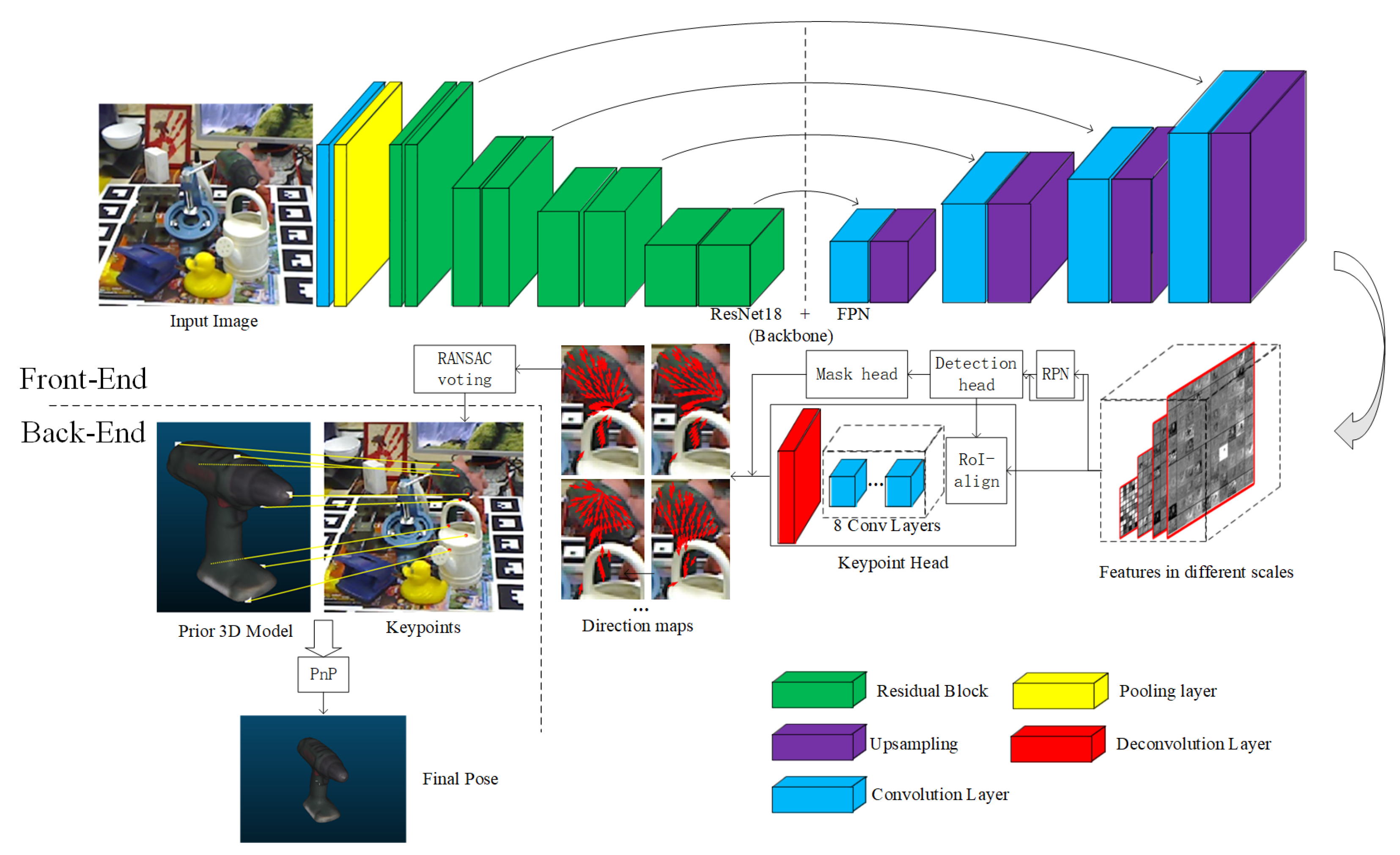
Figure 1. The structure of the network for keypoint estimation.
Applsci 11 00743 g001
Figure 2. Ape.
Figure 2. Ape.
Applsci 11 00743 g002
Figure 3. Cat.
Figure 3. Cat.
Applsci 11 00743 g003
Figure 4. Driller.
Figure 4. Driller.
Applsci 11 00743 g004
Figure 5. Duck.
Figure 5. Duck.
Applsci 11 00743 g005
Figure 6. Local perception for keypoints.
Applsci 11 00743 g006
Figure 7. Comparison between predicted and ground truth pose.
Applsci 11 00743 g007
Table 1. Test results of accuracy on LINEMOD.
Two-StageEnd-to-End
RPVNetHeatmapTekin [16]BB8 [19]Cull [17]PVNet [29]Deep6D [10]SSD-6D [12]
Ape55.642.021.640.455.143.638.8-
Benchvise98.792.781.891.889.099.971.2-
Cam83.682.236.655.766.286.852.5-
Can93.291.368.864.189.295.586.1-
Cat75.573.141.862.675.379.366.2-
Driller94.791.063.574.488.696.482.3-
Duck63.551.427.244.341.852.632.5-
Eggbox95.894.669.657.897.199.279.4-
Glue93.489.880.041.294.695.763.7-
Hole82.579.542.667.268.981.956.4-
Iron96.191.974.984.790.998.965.1-
Lamp96.894.771.176.594.299.389.4-
Phone91.588.547.754.067.692.465.0-
Average86.181.755.962.778.386.465.276.3
Std-Dev15.618.920.516.117.318.317.2-
Wilcoxon t -YesYesYesYesNoYes-
Table 2. Test results of accuracy on Occlusion LINEMOD.
Two-StageEnd-to-End
RPVNetHeatmapTekinOberweger [25]PVNetPoseCNN [11]
Ape17.99.82.4817.615.89.6
Can69.549.317.553.963.345.2
Cat19.011.60.73.316.70.93
Duck31.120.71.119.225.219.6
Driller63.748.17.762.465.641.4
Eggbox59.230.3-25.950.222.0
Glue46.638.510.139.649.638.5
Holepuncher42.828.75.4521.339.622.1
Average43.729.66.430.440.824.9
Std-Dev19.815.15.9919.919.715.7
Wilcoxon t -YesYesYesYesYes
Table 3. Test results of accuracy on Truncation LINEMOD.
ApeBenchiviseCamCanCatDrillerDuckEggbox
PVNet12.842.827.732.925.237.012.444.1
RPVNet14.141.727.332.624.937.214.843.5
GlueHoleIronlampPhoneAverageStd-DevWilcoxon t
PVNet38.122.442.040.930.931.59.5No
RPVNet38.423.240.938.830.031.310.4-
Publisher’s Note: MDPI stays neutral with regard to jurisdictional claims in published maps and institutional affiliations.