Simulation of Crack Propagation in Reinforced Concrete Elements

Abstract

The crack widths in reinforced concrete structures are affected by various influencing parameters, such as the tensile strength of the concrete, which is a highly variable parameter. While safe predictions of crack widths are possible with the existing models supplied in the code provisions accompanied by suitable safety factors, there are large discrepancies between the experimentally measured crack widths and the calculated values. Even within a uniaxial tensile test on reinforced concrete components, several crack parameters (spacings and widths) are usually measured. To further investigate the effects of scattering input parameters on the distribution of crack parameters, a crack propagation model (CPM) is developed, which is a powerful tool that can be used to observe sequential cracking of uniaxially loaded reinforced concrete components. In the present paper, the background of the scattering of the concrete tensile strength will be explained and the procedure for the simulation in the CPM, including the investigation of different bond–slip relationships, will be introduced. Finally, the CPM will be used to calculate experimental crack parameters and the distribution of the calculated crack parameters will be discussed.

1. Introduction

In reinforced concrete structures, cracks are unproblematic, as long as the crack widths are limited to a specific level depending on the environmental conditions. For this purpose, crack width verification is carried out in the design of a structural component, which ensures the requirements are met in terms of the serviceability and durability of the structural component by means of a normatively defined calculated value of the crack width. Different calculation models exist in the respective standards that can be used to verify the calculated crack width, which are nowadays usually mechanically based. Essential differences in the models result from the reference values used for the crack width. In some models, the mean value of the crack widths is used as a reference value and the characteristic crack width is determined using a corresponding increase factor. A further group of models directly calculate the characteristic crack widths. For the comparison of such characteristic crack widths with the measured crack widths in the tests, statistical considerations are required. The 95th percentile of the distribution is associated with the characteristic crack width value. Therefore, for both procedures, sufficient knowledge of the stress-dependent crack formation process is required, as well as knowledge of the resulting scattering and distribution density of the occurring crack widths and crack spacings.

The experimental determination of the stress-dependent crack width distribution is associated with a very high experimental effort, because uniaxial tension tests on long reinforced concrete specimens are required, in which a statistically relevant number of cracks emerge. Such tests were carried out in the 1960s (e.g., [1,2]) and provided a good data basis for structural elements with steel reinforcement and the common concrete properties at that time. For new concrete mixtures, high reinforcement ratios, large-diameter steel bars, or modern non-metallic reinforcement, the amount of available data on existing tests for the statistical distribution of crack parameters (i.e., crack spacing and crack widths) is very limited or does not even exist.

An alternative approach involves the use of numerical models of the crack formation process involving a consistent mechanical background. The performance and prediction accuracy of such models must be proven via validation with experimental tests. In [3,4], efficient models of the simulation of random crack formation have already been developed, which were each developed and used for specific tasks. For more comprehensive considerations of crack formation in reinforced tensile components or flexural tension zones [5], a crack propagation model (CPM) was developed, with the ability to determine the distribution functions of crack widths and crack spacings in a general form.

In this paper, the model setup and features of the CPM are explained and a comparison with experimental tests is carried out for deformed bars. Furthermore, possible extensions of the CPM for investigation of the crack parameters of recently used concrete mixtures (e.g., steel-fiber-reinforced concrete, high-strength concrete, carbon concrete) are presented.

2. General Crack Propagation

If an uncracked reinforced concrete specimen (uncracked stage) is subjected to a steadily increasing centric tensile load, cracks will appear at the point of the lowest concrete tensile strength (initial cracking stage). In the crack, the concrete strain value is zero and the steel strain value is maximal. Due to the bond stresses activated on both sides of the crack, tensile stresses are introduced into the concrete and the steel tensile stresses are reduced until the steel and concrete strains are identical again at the end of the transmission length l_t (Figure 1). With a further increase of the load, the next crack occurs in the remaining uncracked component zone at the point with the lowest concrete tensile strength (crack formation stage; Figure 1, stage 2). This process is repeated until at no point are the steel and concrete strains identical. At this point the stabilized cracking stage is reached (Figure 1, stage 3), however it must be noted that with further load increase beyond this state, further cracks can form.

The crack width in the crack formation stage results from the integration of the strain differences between the reinforcement and surrounding concrete over the transmission length on both sides of the observed crack. In the stabilized cracking stage, the crack width is determined by integrating the strain difference over half of the crack spacing on both sides of the considered crack.

Hence, the concrete tensile strength values (specifically the lower concrete tensile strength values) over the length are significant in terms of initiation of cracks, while the bond–slip behaviour is the major parameter affecting the transmission of stresses between the steel bar and the concrete. Therefore, to simulate the whole crack propagation process with increasing load level (i.e., increasing steel stress ${\sigma }_{\mathrm{s}}$), the crack propagation model (CPM) is configured with the following features:

• For random cracking, concrete tensile strength scattering along the longitudinal axis of the specimen is required. Therefore, the CPM can map different statistical distributions;
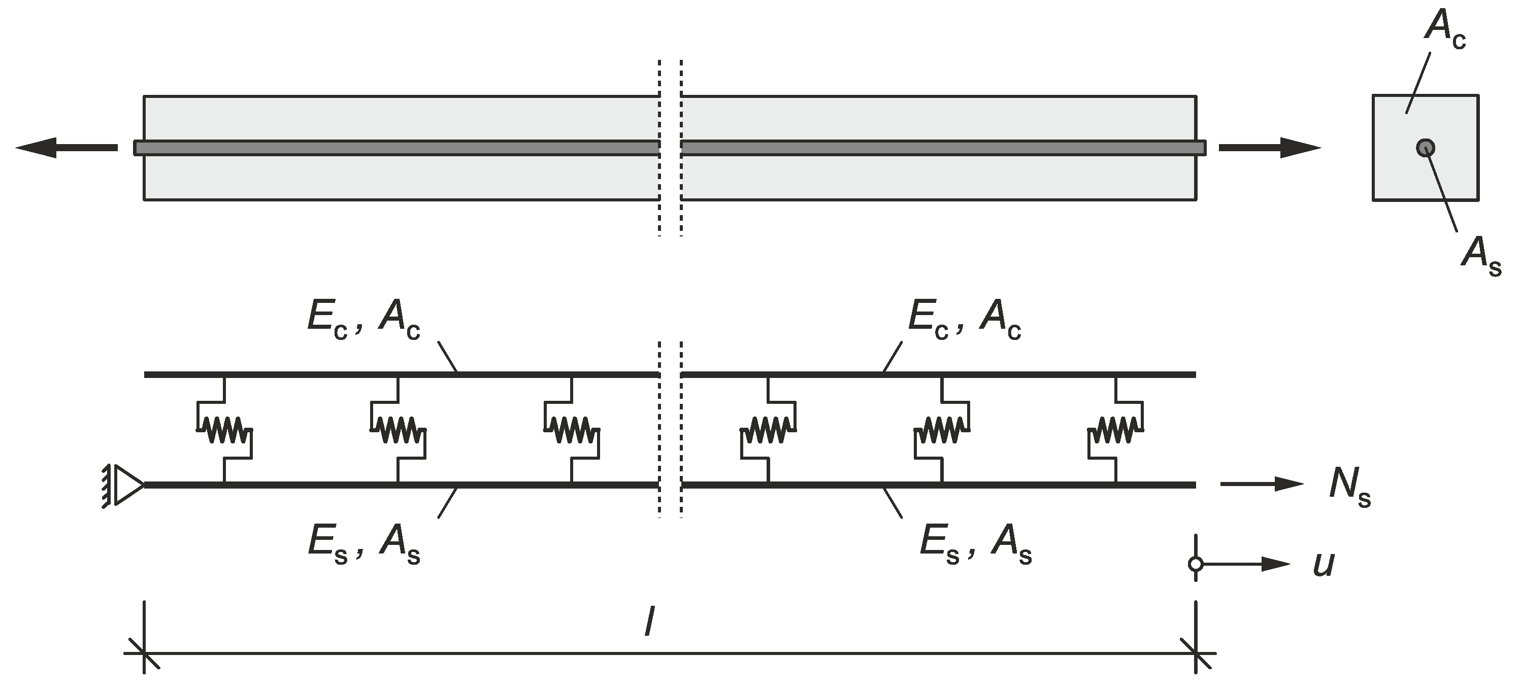
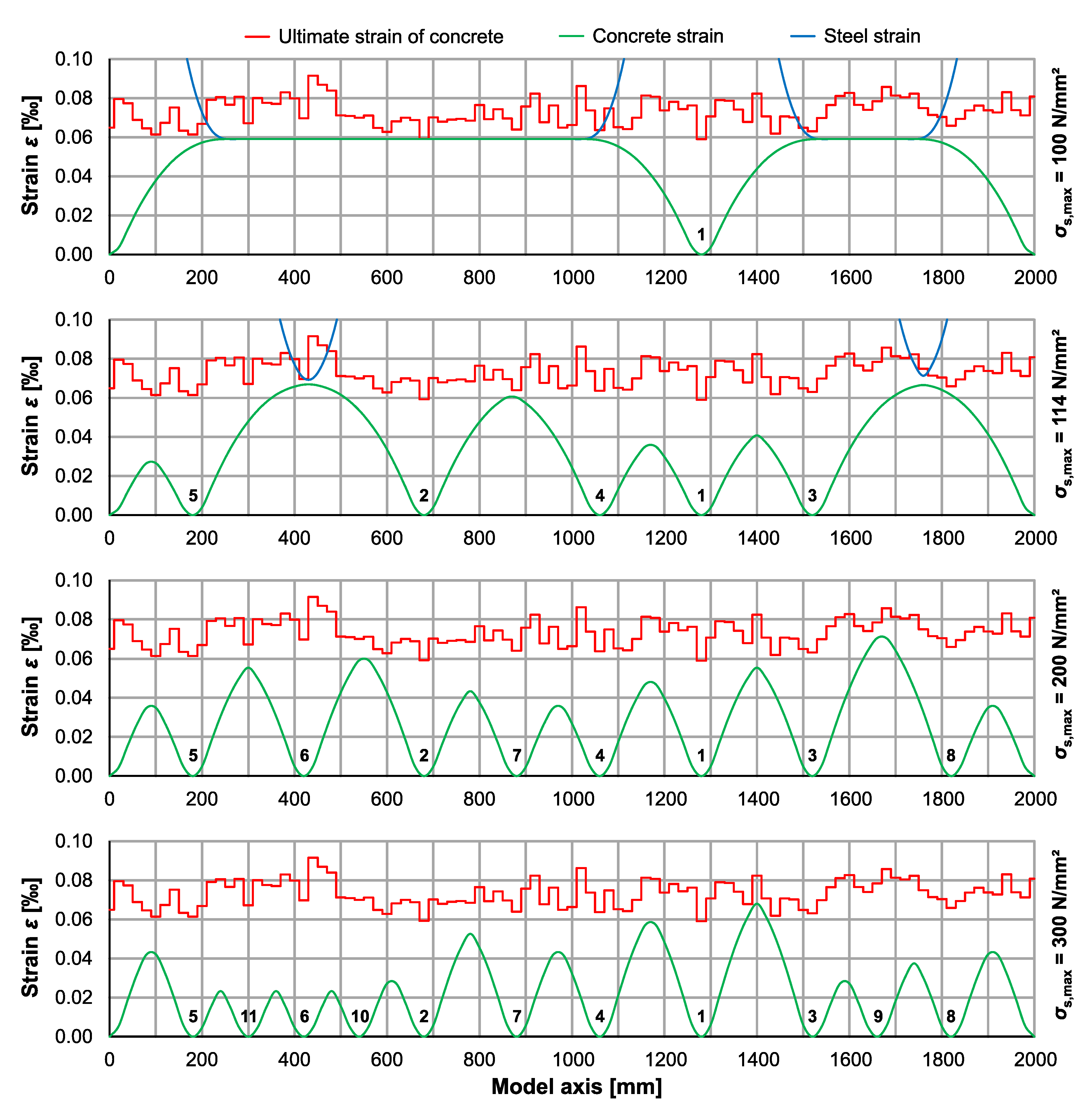
• It must be possible to calculate steel and concrete strains separately over the entire length of the specimen. Thus, both materials shall be represented separately;
• A bond stress–slip relationship is required for the interaction of both materials. This should be definable in a general mathematical form to be able to take into account different loading levels and material configurations.

Using these features, the crack formation can be considered in a very variable and specific way (e.g., through adaptation of input parameters and calculation steps and isolated consideration of influence parameters with almost any number of calculation runs). Using a random definition for the concrete tensile strength over the specimen length, the random locations of the crack initiation and random crack spacings can be determined. Furthermore, the statistical distribution of the output crack widths and crack spacings can be investigated with several runs and numerous random parameters within a specific range.

However, to obtain a mechanically reasoned model with very good prediction accuracy, specific considerations concerning the tensile strength distribution are needed to reach element-size-independent and reasonable results. Such aspects of the CPM model will be explained in the following.

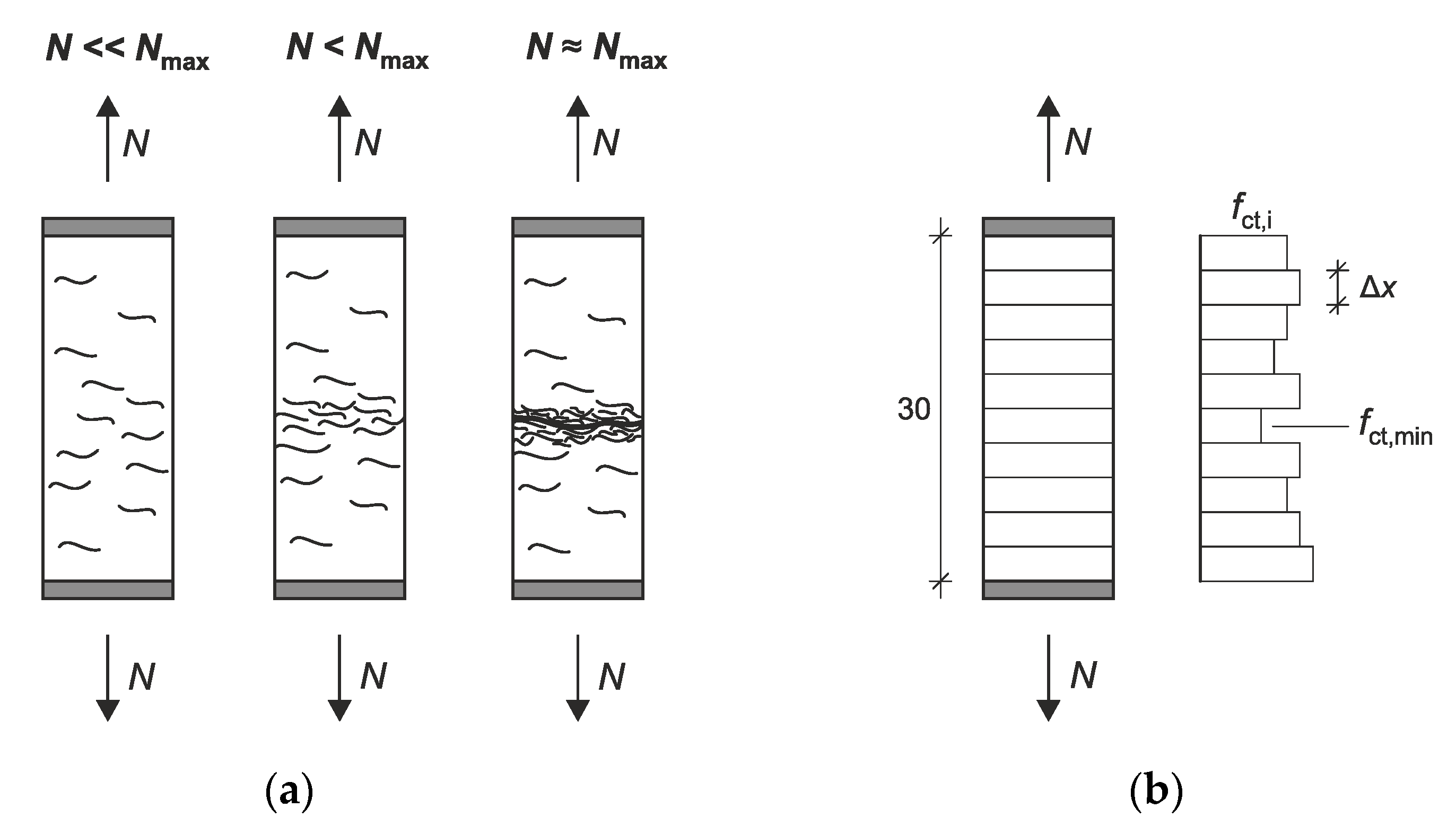
3. Crack Propagation Model (CPM)

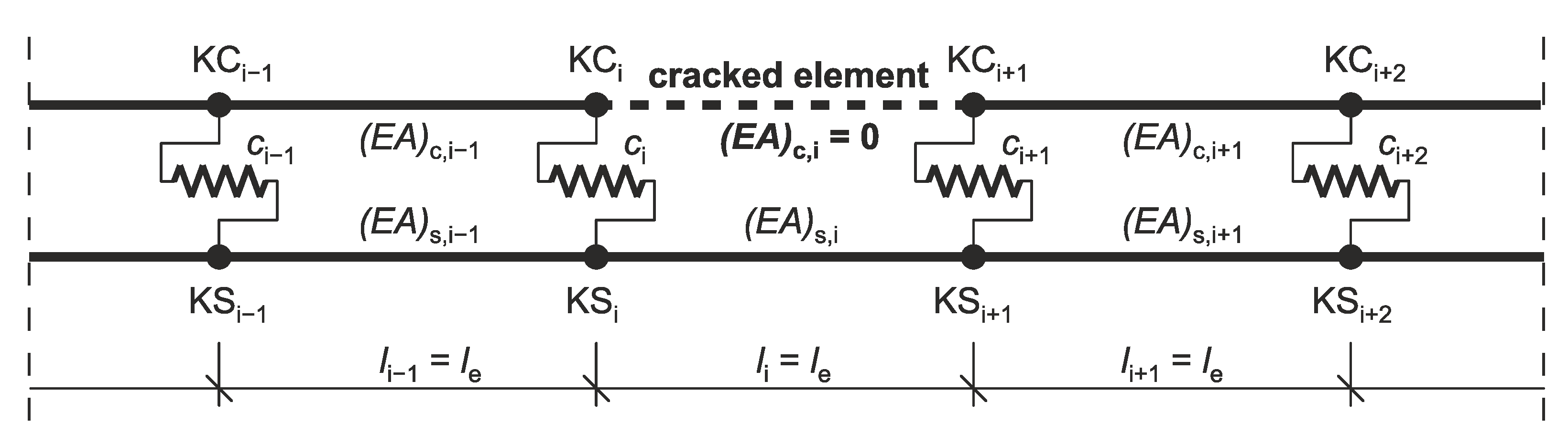
3.1. Model Setup

To implement the features listed in the previous section, the rheological model described in [6,7] was extended. The basic model consists of two uniaxial bars (concrete and reinforcing steel), which are connected with springs at a defined distance (Figure 2). Here, the springs represent the bond between the steel bar and the concrete bar. The extended crack propagation model (CPM) allows “free crack formation” of the concrete tensile strength scattering along the bar or component axis (cf. models in [3,4]). The scattering of the concrete tensile strength is randomly generated according to a given distribution (e.g., normal distribution, logarithmic normal distribution).

In contrast to the rheological model in [6,7], the specified model length l of the CPM corresponds to the entire length of the simulated component. The crack formation is recorded via stiffness reduction of the corresponding concrete element (EA)_c,I = 0 (Figure 3).

Since a crack can only emerge between two nodes, i.e., in the middle of a concrete bar element (Figure 3), the crack width is calculated by using the slip difference of the left and right nodes, taking into account the steel bar strains. Considering that the strain values in the remaining “concrete stumps” (between concrete nodes KC_i and KC_i+1) equal zero and the steel strain values in the steel bar element i (between steel nodes KS_i and KS_i+1) correspond to ε_s,i = (u_KS,i+1 − u_KS,i) ⁄ l_i, the calculated crack width can be simplified as the difference between the translation u of the concrete nodes KC_i+1 and KC_i:

$$\begin{array}{c}{w}_{\mathrm{cal},\mathrm{i}}=s_{\mathrm{i}}- s_{\mathrm{i}+1}+{\epsilon }_{\mathrm{s},\mathrm{i}}·l_{\mathrm{i}}\\ =\left(u_{\mathrm{KS},\mathrm{i}}-u_{\mathrm{KC},\mathrm{i}}\right)-\left(u_{\mathrm{KS},\mathrm{i}+1}-u_{\mathrm{KC},\mathrm{i}+1}\right)+{\epsilon }_{\mathrm{s},\mathrm{i}}·l_{\mathrm{i}}\\ =u_{\mathrm{KC},\mathrm{i}+1}-u_{\mathrm{KC},\mathrm{i}}\end{array}$$

(1)

where s_i is the slip at node i; u_KS,i is the translation of the steel bar at node i; u_KC,i is the translation of the concrete bar at node i; ε_s,i is the strain of the steel bar i; and l_i is the length of element i.

Using such simplified linear displacement methods, the element size should be selected carefully to obtain reasonable results. In the CPM, the error of the determined crack widths is usually less than 3%, with 6 to 8 elements between two cracks. Therefore, the element length l_e is generally selected with regard to the expected crack spacing s_r, which is assumed over a reasonable range for the investigated specimen (e.g., considering the reinforcement ratio, rebar diameter, and bond–slip relationship).

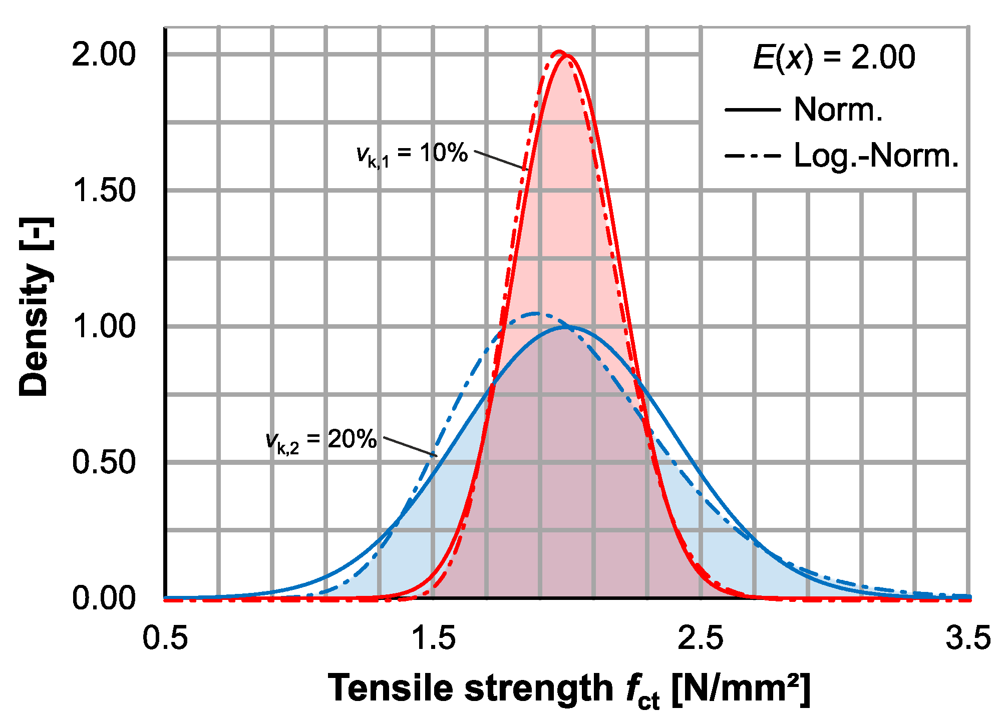
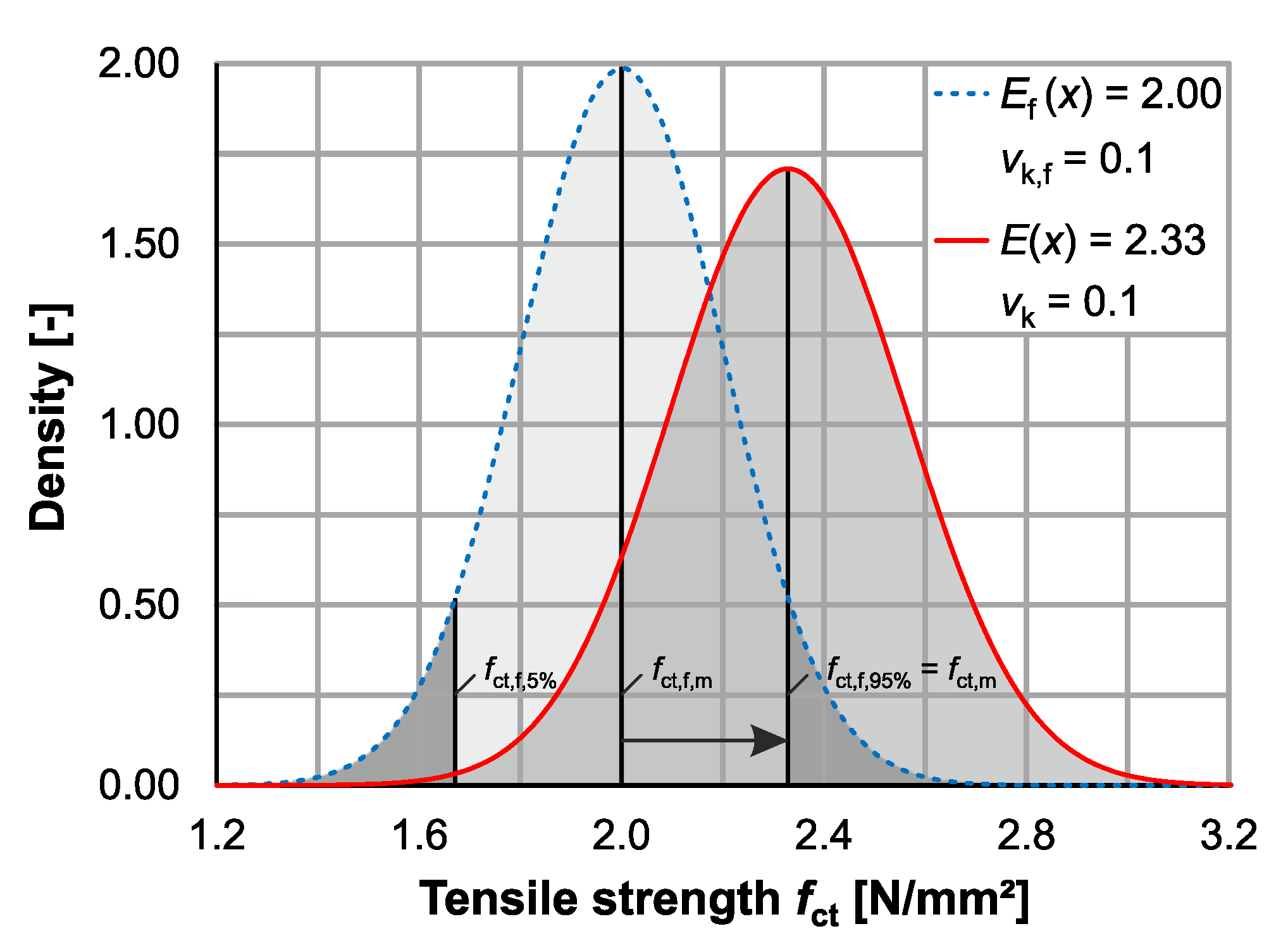
3.2. Distribution of Tensile Strength

The experimental determination of tensile strength has been the subject of recent research (e.g., [8,9]), and several indirect and direct testing methods exist. Uniaxial concrete tensile strength is determined most effectively using a direct (uniaxial) tensile test (Figure 4). To determine the scattering of the concrete tensile strength of a single batch, the statistical distribution of several direct tensile tests is required. This scattering is caused by a wide variety of reasons, such as flaws due to insufficient compaction, the presence of inhomogeneity and anisotropy caused by aggregates, as well as internal stress states caused by shrinkage and hydration of cement.

To describe the distribution of tensile strength, a probability function is required. In [10], a logarithmic normal distribution is assumed. In contrast, [11] and some codes in [12,13] assume a normal distribution, while a summary is provided in [14]. Both distributions are shown in Figure 5 (probability density function) for an expected tensile strength value of 2.0 N/mm² and coefficients of variation of v_k,1 = 10% and v_k,2 = 20%.

It can be seen that both distributions are very similar for a coefficient of variation v_k,1 = 10%, with an overlap of 96.2%. For v_k,2 = 20%, the overlap is 92.4%, but the visible deviation in Figure 5 is significantly larger than for v_k,1 = 10%. Consequently, the logarithmic normal distribution for v_k < 20% can be approximately represented by a normal distribution.

For ranges of variation for different expected values, a distinction must be made between a constant standard deviation and a constant coefficient of variation. For the concrete tensile strength—in contrast to the concrete compressive strength (standard deviation constant [15,16])—the coefficient of variation is considered a constant quantity. With regard to the scattering of the tensile strength at failure, evaluations in [11,17,18] show a coefficient of variation v_k < 10%. In Model Code 2010 [12] and Eurocode 2 [13], the coefficient of variation of the tensile strength of the component is v_k = 18% (see [4]). Similar results are demonstrated in [19], by considering the influences of different concrete mixtures [17]. Thus, for one concrete batch, a coefficient of variation v_k < 10% seems to be realistic. For several concrete batches in a component or in the absence of tensile tests, v_k = 18% may be reasonable. For the probability function of the tensile strength, however, a normal distribution can be assumed approximately in both cases.

The aforementioned distribution function applies to the tensile strength values obtained from several uniaxial tensile tests and cannot be directly implemented to define a tensile strength distribution in the CPM to simulate a tensile bar. This is due to the fact that in uniaxial tensile tests (of unnotched specimens), the tensile strength applies to the weakest point of the specimen. In the following, this value will be designated as the fracture tensile strength f_ct,f. Previous experimental investigations (e.g., [17,20]) show a difference between the distribution of the tensile strength within a specimen and the distribution of the fracture tensile strength f_ct,f. Regarding this point, Empelmann [3] defined a term for the specimen tensile strength f_ct, which is explained below.

Figure 6a shows the fracture process in a uniaxial tensile specimen. The existing micro-cracks accumulate at the weakest point of the specimen shortly before the maximum load is reached [21]. The minimum tensile strength shown in Figure 6b corresponds to the fracture tensile strength f_ct,min = f_ct,f. Figure 6b schematically shows the tensile strength values in representative elements (which will be discussed later). Based on this point, it is logical that the mean value of all f_ct,i values is higher than the mean value of several f_ct,f values obtained using several uniaxial tensile tests.

Consequently, an adaption is required to derive the distribution of the specimen tensile strength f_ct (all values in a component) based on the given distribution of the fracture tensile strength values f_ct,f (weakest values in a component in uniaxial tensile specimens without a notch).

According to [3], such adaption can be built by assuming a normal distribution for f_ct,f and f_ct and setting the mean value of the specimen tensile strength f_ct,m equal to the 95th percentile value of the fracture tensile strength f_ct,f,95%.

For the mean value of the fracture concrete tensile strength f_ct,f,m = 2.0 N/mm², the following percentile values are obtained by setting the assumed coefficient of variation (of the fracture tensile strength) as equal to v_k,f = 10%:

$$f_{\mathrm{ct},\mathrm{f},5\%}=f_{\mathrm{ct},\mathrm{f},\mathrm{m}}\cdot \left(1-1.645\cdot v_{\mathrm{k},\mathrm{f}}\right)=2.0 \mathrm{N}/{\mathrm{mm}}^2\cdot \left(1-1.645\cdot 0.1\right)=1.67 \mathrm{N}/{\mathrm{mm}}^2$$

(2)

$$f_{\mathrm{ct},\mathrm{f},95\%}=f_{\mathrm{ct},\mathrm{f},\mathrm{m}}\cdot \left(1+1.645\cdot v_{\mathrm{k},\mathrm{f}}\right)=2.0 \mathrm{N}/{\mathrm{mm}}^2\cdot \left(1+1.645\cdot 0.1\right)=2.33 \mathrm{N}/{\mathrm{mm}}^2$$

(3)

The mean value of the specimen tensile strength corresponds to:

$$f_{\mathrm{ct},\mathrm{m}}=f_{\mathrm{ct},\mathrm{f},95\%}=2.33 \mathrm{N}/{\mathrm{mm}}^2$$

(4)

Assuming equal coefficient variations v_k = v_k,f = 10%:

$$f_{\mathrm{ct},\mathrm{m},5\%}=f_{\mathrm{ct},\mathrm{m}}\cdot \left(1-1.645\cdot v_{\mathrm{k}}\right)=2.33 \mathrm{N}/{\mathrm{mm}}^2\cdot \left(1-1.645\cdot 0.1\right)=1.95 \mathrm{N}/{\mathrm{mm}}^2$$

(5)

$$f_{\mathrm{ct},\mathrm{m},95\%}=f_{\mathrm{ct},\mathrm{m}}\cdot \left(1+1.645\cdot v_{\mathrm{k}}\right)=2.33 \mathrm{N}/{\mathrm{mm}}^2\cdot \left(1-1.645\cdot 0.1\right)=2.71 \mathrm{N}/{\mathrm{mm}}^2$$

(6)

where f_ct,f,m is the mean value of the fracture tensile strength; v_k,f is the coefficient of variation of the fracture tensile strength; f_ct,m is the mean value of the specimen tensile strength; v_k is the coefficient of variation of the specimen tensile strength; 5% is the 5th percentile value; and 95% is the 95th percentile value.

This calculation method is depicted in Figure 7.

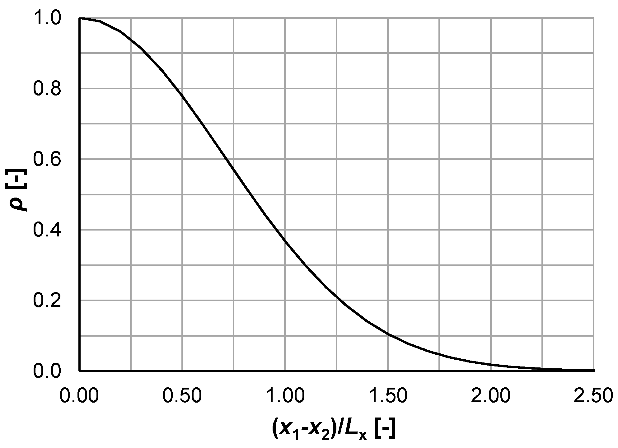
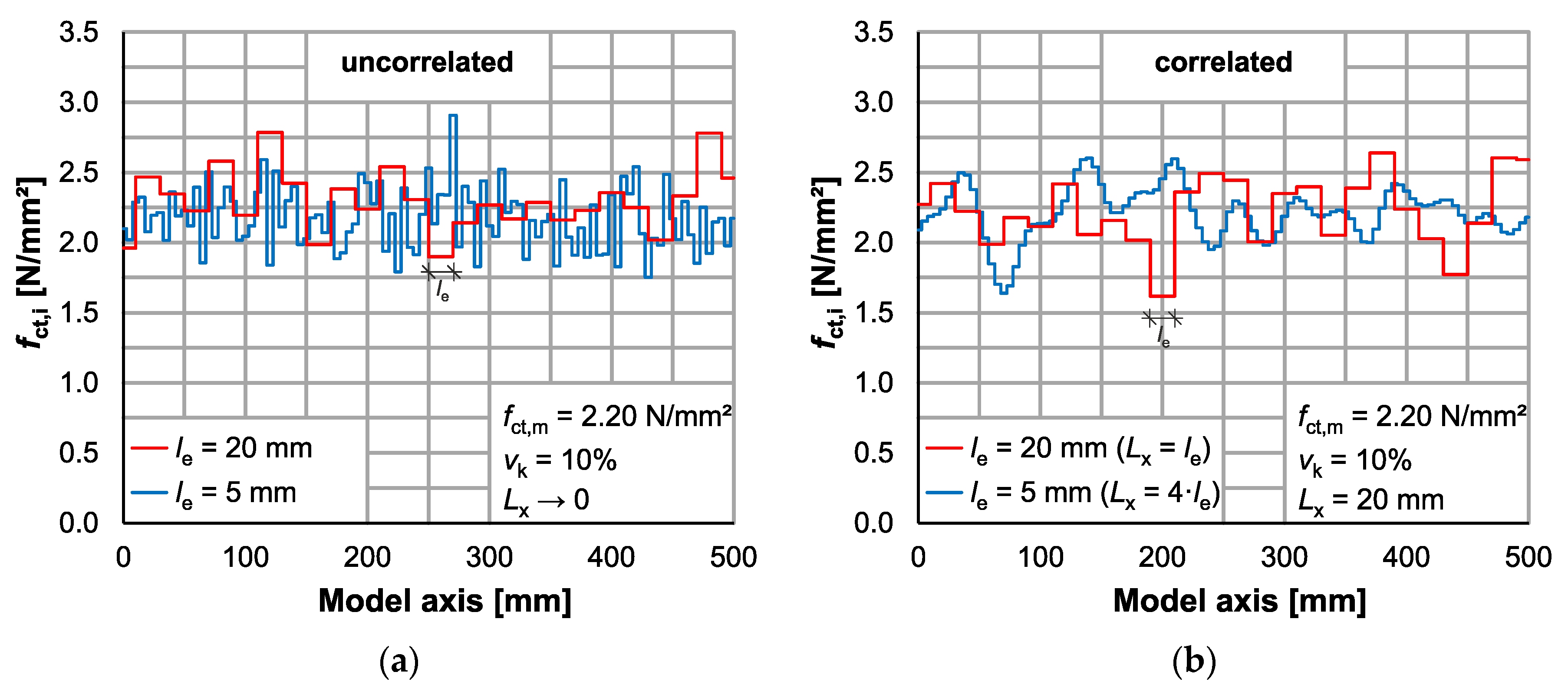
3.3. Element Size and Autocorrelation

The concrete bar of the CPM consists of a finite elements series, with each element being assigned a random tensile strength f_ct,i according to the applied distribution. As shown in Section 3.2 (Figure 6), each tensile strength value is assigned according to a mechanically reasoned representative element size ∆x, which is often defined based on the maximum aggregate size d_g. Here, ∆x is assumed to be in the range of 2·d_g to 3·d_g [3,22,23]. A maximum aggregate size of 16 mm results in a representative element size ∆x of about 32–48 mm. The element size affects directly the prediction accuracy of the model and the accuracy of the crack spacing values, as a crack can only emerge in the mid-length area of each element. Therefore, to enable the simulation of fine cracking patterns, the element length l_e should also be very small. To consider these aspects and simultaneously achieve a nearly mesh-independent model, a smaller element length l_e is selected and the concrete tensile strengths of the adjacent elements within a correlation length L_x are correlated to avoid mechanically inconsistent oscillation of the tensile strengths in the smaller elements. This approach is known as spatial autocorrelation [24].

The expression of the linear dependence or correlation between two points x₁ and x₂ is described by the correlation function ρ(x₁,x₂). A common form is the quadratic exponential (Gaussian) correlation function [4,25,26].

$$\rho \left(x_1,x_2\right)=e^{-{\left(\frac{\left|x_1-x_2\right|}{L_{\mathrm{x}}}\right)}^2}$$

(7)

Figure 8 illustrates the correlation function according to Equation (7). For ρ(x₁,x₂) = 0, there is no linear correlation between x₁ and x₂, whereas ρ(x₁,x₂) = 1 shows a full dependency of both points.

By multiplying the correlation function with the standard deviations σ(x₁) and σ(x₂) (here σ(x₁) = σ(x₂) = σ), the value of covariance is obtained and the positive symmetric covariance matrix C can be composed:

$$\mathit{C}=\left[\begin{array}{cccc}{\sigma }^2& {\rho }_{12}{\sigma }^2& \cdots & {\rho }_{1\mathrm{n}}{\sigma }^2\\ {\rho }_{21}{\sigma }^2& {\sigma }^2& \cdots & {\rho }_{2\mathrm{n}}{\sigma }^2\\ ⋮& ⋮& \ddots & ⋮\\ {\rho }_{\mathrm{m}1}{\sigma }^2& {\rho }_{\mathrm{m}2}{\sigma }^2& \cdots & {\sigma }^2\end{array}\right]$$

(8)

The generation of normally distributed correlated random numbers can be performed by means of the Cholesky decomposition. When using the Cholesky decomposition, normally distributed uncorrelated random values (a₁, a₂, … a_m) with a mean value of zero and a standard deviation of one must first be generated. These represent the size of the scattering area.

The Cholesky decomposition of the correlation matrix leads to:

$$\mathit{C}=\mathit{L}\cdot {\mathit{L}}^{\mathrm{T}}$$

(9)

Subsequently, the normally distributed random values (a₁, a₂, … a_m) are multiplied with the triangular matrix L:

$$\left[\begin{array}{c}{a}_1^{*}\\ a_2^{*}\\ ⋮\\ a_{\mathrm{m}}^{*}\end{array}\right]=\left[\begin{array}{cccc}{L}_{11}& 0& \cdots & 0\\ L_{21}& L_{22}& \cdots & 0\\ ⋮& ⋮& \ddots & ⋮\\ L_{\mathrm{m}1}& L_{\mathrm{m}2}& \cdots & L_{\mathrm{mn}}\end{array}\right]\cdot \left[\begin{array}{c}{a}_1\\ a_2\\ ⋮\\ a_{\mathrm{m}}\end{array}\right]$$

(10)

This results in a normally distributed correlated distribution, which must be added to the mean value of the desired distribution (here this is f_ct,m) [25,27]:

$$f_{\mathrm{ct},\mathrm{i}}=f_{\mathrm{ct},\mathrm{m}}\cdot \left(1+a_{\mathrm{i}}^{*}\right)$$

(11)

As laid out before, L_x should be defined in order to give a meaningful correlation by considering the representative element size and so as to generate a good dependency with regard to the correlation function at the same time. According to the correlation function in Figure 8, there is almost no correlation in the case of l_e/L_x = 2. This means that almost uncorrelated random values are generated for L_x = l_e/2. Based on Section 3.2, this should be valid for a representative element size ∆x of 2·d_g to 3·d_g. Therefore, the correlation length can subsequently be assumed according to:

$$1.0\cdot d_{\mathrm{g}}\le L_{\mathrm{x}}\le 1.5\cdot d_{\mathrm{g}}$$

(12)

which means a correlation length L_x of between 16 and 24 mm for an aggregate size d_g = 16 mm.

Figure 9 illustrates the influence of the correlation length for uncorrelated and correlated distributions of the tensile strength along the model axis for element sizes of 5 and 20 mm. All distributions are generated randomly according to the values specified in Figure 9. For uncorrelated values, the distribution of l_e = 5 mm has too many local minima and maxima compared to l_e = 20 mm. The distributions along the axis are not comparable (although the probability density functions are almost the same), leading to a mesh dependency. In the case of correlated values, there is almost no mesh dependency, as the numbers of local minima and maxima are similar for l_e = 20 mm and l_e = 5 mm.

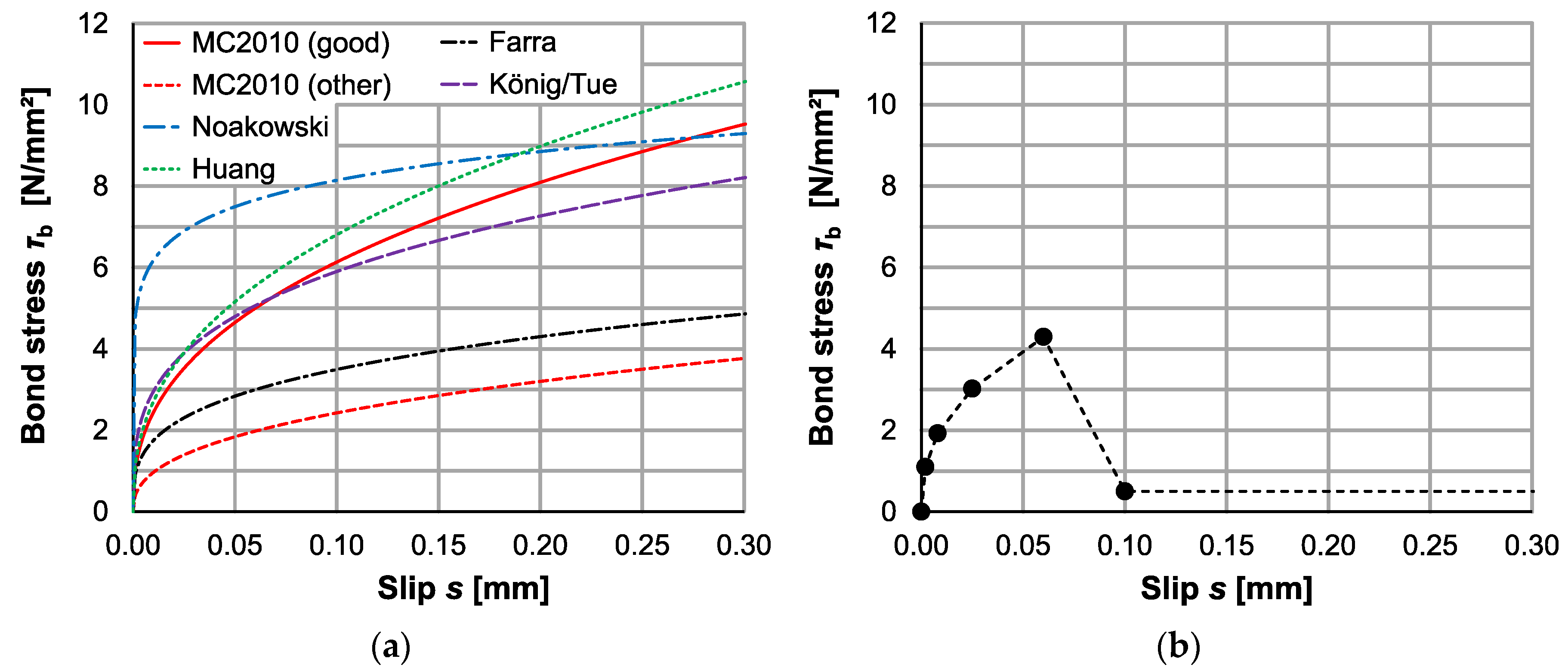
3.4. Bond–Slip Relationship

The bond–slip behaviour between the concrete bar and reinforcement bar is simulated in the CPM using springs with a stiffness equal to:

$$\mathrm{c}=\left({\tau }_{\mathrm{b}}\left(s\right)/s\right)\cdot u_{\mathrm{s}}\cdot l_{\mathrm{e}}$$

(13)

where τ_b(s) is the local bond stress; s is the local slip (relative displacement between concrete and rebar); u_s is the perimeter of the reinforcement bar; and l_e is the element length.

A bond–slip relationship according to Equation (14) is chosen in the first instance, with which a large variety of bond laws can be integrated:

$${\tau }_{\mathrm{b}}\left(s\right)={\tau }_{\mathrm{b},\max }\cdot {\left(\frac{s}{s_1}\right)}^{\mathsf{\alpha }}$$

(14)

This correlation corresponds to the ascending branch of the bond law according to Model Code 2010 [12]. For calculations in the serviceability limit state, using the ascending branch of the bond–slip relationship is sufficient according to [28]. This considers the expected maximum crack width of 0.4 mm, which corresponds to a slip of 0.2 mm at both sides of the cracks, which is clearly within the ascending branch of the bond–slip relationship.

For the general form of the bond–slip relationship according to Equation (14), some reference values based on the technical literature are listed in

Table 1. Parameters for the ascending branch of the bond–slip relationship for normal-strength concrete.

Model	Bond Conditions	τb,max	s1	α
MC2010 [12]	Good	$2.5\cdot \sqrt{f_{\mathrm{cm}}}$	1.0	0.40
MC2010 [12]	All other cases	$1.25\cdot \sqrt{f_{\mathrm{cm}}}$	1.8	0.40
Farra [29]	Mean	$0.22\cdot f_{\mathrm{cm}}^{0.95}$	1.0	0.30
König and Tue [30]		$0.31\cdot f_{\mathrm{cm}}$	1.0	0.30
Noakowski [31]	Good	$0.95\cdot f_{\mathrm{cm}}^{2/3}$	1.0	0.12
Huang [32]	Good	$0.45\cdot f_{\mathrm{cm}}$	1.0	0.40

and are illustrated in Figure 10a for concrete strength class C30/37.

Even if the real bond behaviour differs significantly from the bond–slip relationship in Equation (14), user-defined bond–slip relationships can be defined in the CPM using slip values and the corresponding bond stress values. Between the points, a linear interpolation is used to determine the missing values. The only prerequisite here is the starting point at the coordinate origin (τ_b(s = 0) = 0). An exemplarily user-defined bond–slip relationship is shown in Figure 10b for a splitting failure.

A reduction of the local bond stress in the vicinity of a separation crack, e.g., due to internal cracking, can be considered by using a linear reduction factor according to [12]:

$${\tau }_{\mathrm{b},\mathrm{red}}\left(\mathrm{s},x\right)=\mathsf{\lambda }\left(x\right)\cdot {\tau }_{\mathrm{b}}\left(s\right)$$

(15)

where: λ(x) is the factor for a reduction of the local bond stress at distance x from the separation crack; x is the distance from the crack; and τ_b(s) is the local bond stress (e.g., according to Equation (14)).

In Model Code 2010 [12], λ(x) is defined by:

$$\mathsf{\lambda }\left(x\right)=0.5\cdot x/\varphi \le 1.0$$

(16)

As an alternative to the linear reduction factor according to Equations (15) and (16), it is also possible to take into account the zone of the disturbed bond using a regionally separated bond stress–slip relationship according to [33,34,35]. It must be noted that the numerical calculation effort and the computation time increase significantly with the used model.

3.5. Model Features and Advantages

The model is characterized by its fast and stable calculation of cracking. In addition, the CPM is easily extendable, e.g., to simulate cracking of fiber-reinforced concrete (FRC) by considering the fiber effects as a crack-width-dependent additional element load. Furthermore, simulation of high-performance concrete (HPC)and ultra-high performance concrete (UHPC) is possible by setting the properties of the concrete bar and adjusting the bond–slip relationship. Additionally, an extension to a three-bar model (see Figure 11) is possible, which enhances the simulation of elements with different reinforcing elements (e.g., elements with prestressed conventional steel rebars). Non-metallic reinforcement (such as carbon concrete, basalt, or glass fiber reinforcements) can be accommodated by adjusting the material parameters of the “reinforcement bar” and the bond–slip relationship. By adjusting the support conditions, constrained stresses can also be investigated. A transfer to components subjected by flexure is possible if the tension and compression zone are treated separately [5].

In addition to the listed expansion possibilities for different materials, the CPM can be expanded with regard to the scattering of the material parameters. In particular, the scattering of the bond stress should be mentioned here. Other scattering parameters (e.g., the modulus of elasticity of the rebar and concrete) are expected to be less significant or can be represented by already existing scattering parameters (e.g., scattering dimensions of the concrete bar by scattering of the tensile strength, scattering diameter of the rebar by scattering of bond stress).

4. Simulation and Calculation Procedure

With the preceding explanations, the CPM can be used to simulate the cracking of a reinforced concrete tensile specimen. In the following, the programme sequence will be briefly explained. A representation can be taken from Figure 12.

In the first calculation step, the entire model or component is uncracked. A load increase follows until the concrete tensile strength is exceeded at the “weakest” point. Then, the stiffness of the cracked concrete element is reduced to zero ((EA)_c,i = 0) (also see Figure 3). The model is recalculated with the adjusted stiffness value (cracked concrete element). The load is then increased further until the concrete tensile strength is exceeded at another point. The process is repeated until the desired load level N_s,end is reached.

The iterative calculation procedure in the CPM will be illustrated below using an example. The calculations are based on the parameters listed in

Table 2. CPM parameters for the case example.

Geometry
Reinforcement ratio	ρ	2%
Diameter of reinforcing bar	∅	16 mm
Length of model	l	2000 mm
Element length	le	20 mm
Material
Concrete: C20/25
Mean value of compressive strength of concrete	fcm	28 N/mm2
Mean value of tensile strength of concrete	fct,m	2.2 N/mm2
Mean value of modulus of elasticity of concrete	Ecm	30,000 N/mm2
Reinforcement: B500
Modulus of elasticity of reinforcing steel	Es	200,000 N/mm2
Bond–slip relationship
Model Code 2010 (good bond conditions)
Bond stress	${\tau }_{\mathrm{b}}\left(s\right)=13.23\cdot {\left(s/1.0\right)}^{0.4}$
Reduction factor	$\mathsf{\lambda }\left(x\right)=0.5\cdot x/16\le 1.0$
Scattering
Tensile strength of concrete
Coefficient of variation	vk	10%
Correlation length	Lx	20 mm

.

Figure 13 shows the strains determined with the CPM for different load levels (expressed by the maximum steel stress σ_s,max). At the cracks, the concrete stress is zero. The first crack occurs with a steel stress of σ_s,max = 100 N/mm² at the point of lowest concrete tensile strength, depending on the distribution of the specimen tensile strength (for comparison, without scattering of the concrete tensile strength v_k = 0, cracking would not occur until σ_s,max = 125 N/mm²). Outside the transmission length, the steel and concrete stresses between the cracks are identical until the completed crack pattern with σ_s,max = 114 N/mm² is reached. Up to this loading level five cracks are formed, mainly at the low points of the strength distribution. Due to the non-linear bond law, a further increase in the load level leads to an increase in the bond forces, and thus also to a greater introduction of force into the concrete. This leads to further cracking occurring in the stabilized cracking stage (progressive stabilized cracking). These cracks predominantly occur centrally between the existing cracks, so that under certain circumstances, regions with higher strength values are also affected by crack formation, i.e., “late” cracks can emerge under relatively high stresses.

The individual crack spacing and crack widths for each stress level can then be read out from the CPM calculation results. If several calculation runs are carried out with the newly generated specimen tensile strength distributions along the model axis in each case, extensive distributions of crack spacing and crack widths can be generated as functions of the stress level and a large data basis can be obtained. In contrast to the stages defined in Figure 1, the switch between crack formation stages and the stabilized cracking stage is quite smooth. Hence, stress regions causing fast crack formation can be identified.

5. Comparison with Experiments

The performance of the CPM will be demonstrated in the following using a series of tests from [36]. The test series included three identical large-scale tests. The focus of the tests was on the generation of many cracks and investigation of the crack spacing distribution. For this purpose, a very high reinforcement ratio of ρ = 8% with a bar diameter of 32 mm was chosen. A tensile force of 900 kN was required to reach a stress level of σ_s,max = 280 N/mm². Figure 14 shows the geometrical parameters of the test specimens used in [36].

The material parameters of the concrete were determined in [36] using compression tests and splitting tensile tests (no data available on scattering). The maximum aggregate size was 16 mm. The parameters used in the CPM are listed in

Table 3. CPM parameters for the test series conducted by Naotunna [36].

Geometry
Reinforcement ratio	ρ	8%
Diameter of reinforcing bar	∅	32 mm
Length of model	l	2000 mm
Element length	le	10 mm
Material
Concrete
Mean value of compressive strength of concrete	fcm	35 N/mm2
Mean value of tensile strength of concrete	fct,m	3.2 N/mm2
Mean value of modulus of elasticity of concrete	Ecm	32,000 N/mm2
Reinforcement: B500
Modulus of elasticity of reinforcing steel	Es	200,000 N/mm2
Bond slip relationship
Model Code 2010 (good bond conditions)
Bond stress	${\tau }_{\mathrm{b}}\left(s\right)=14.79\cdot {\left(s/1.0\right)}^{0.4}$
Reduction factor	$\mathsf{\lambda }\left(x\right)=0.5\cdot x/32\le 1.0$
Scattering
Tensile strength of concrete	18 distributions (in each case)
Coefficient of variation	vk	10% (15%)
Correlation length	Lx	20 mm (10 mm)

. A correction of the tensile strength according to Section 3.2 was not performed, as splitting tensile tests were conducted (here f_ct,f,m = f_ct,m).

The calculations were first carried out for a coefficient of variation of v_k = 10% and a correlation length of 20 mm (~1.25 d_g, cf. Equation (12)). In a second calculation run, a correlation length of 10 mm was applied for comparison and to consider the small crack spacings. To account for the uncommonly high reinforcement ratio and large reinforcement diameter in combination with the relatively small crack spacing, a coefficient of variation of v_k = 15% was also applied. Since in [36] the crack spacing was recorded on 3 sides at the depths of each reinforcement layer (3 specimens × 3 surfaces × 2 bars = 18 sets), 18 generated distributions were recorded for each calculation run. To take the disturbed stress region at loading points into account, both the values presented in [36] and the CPM did not take into account the last crack spacing on both sides of the test specimens.

The distribution of experimental crack spacing and the calculated crack spacing with the CPM is shown in Figure 15a for v_k = 10% and in Figure 15b for v_k = 15%. The statistical parameters are summarized in

Table 4. The statistical parameters from Figure 15.

	Naotunna [36]	CPM: vk = 10%		CPM: vk = 15%
		Lx = 20 mm	Lx = 10 mm	Lx = 20 mm	Lx = 10 mm
Total number n 1	230	214	217	215	224
Mean (section) sr,m	131–140 mm	141–150 mm	141–150 mm	141–150 mm	131–140 mm
Median (section)	121–130 mm	131–140 mm	131–140 mm	131–140 mm	121–130 mm
95th percentile (section) sr,0.95	191–200 mm	191–200 mm	191–200 mm	191–200 mm	181–190 mm
sr,0.95/sr,m	~1.5	~1.4	~1.4	~1.4	~1.4

¹ Recorded crack spacings for 3 specimens, 3 surfaces, and 2 bars each (6 sets per specimen).

. A calculation with twice as many elements (l_e = 5 mm) showed similar results, with the exception of small deviations in the distribution of the crack spacings due to the randomly generated tensile strength distributions.

The comparison of the experimental and calculated crack spacing shows the following results:

• In general, the test results can be reproduced very well with the CPM (see Figure 15 and Table 4);
• Varying the coefficient of variation and correlation length to determine the distribution of the tensile strength along the model axis has only a limited effect on the results;
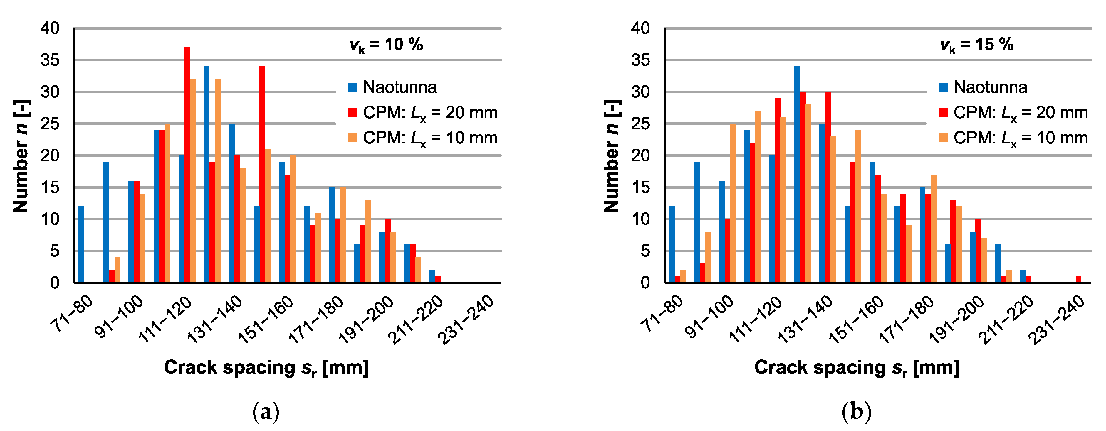
• The range of very small crack spacings ($s_{\mathrm{r}}\le 100 \mathrm{mm}$) is underestimated for v_k = 10% and v_k = 15%, as well as for L_x = 20 mm and L_x = 10 mm (see Figure 15);
• The experimental value s_r,0.95/s_r,m = 1.5 is estimated with adequate accuracy by the CPM (s_r,0.95/s_r,m = 1.4) (see Table 4);
• The comparison of the median and mean values of the experimental results show a positive skew (skewed to the right) (see Table 4) indicating a log-normal distribution of the crack spacing s_r.

The high number of very small crack spacings (s_r ≤ 100 mm) can be attributed to the fact that complete separation cracks do not always form in testing and that overlapping cracks can occur. Both phenomena can be observed in [36]. Furthermore, the effects of shrinkage strains have not been taken into account in the calculation with the CPM, as the respective input values were not documented in [36]. However, the model can consider shrinkage by adding shrinkage strains as an additional load component to reduce the effective tensile concrete strength [6,7]. As a result, the crack spacing would be reduced.

6. Discussion and Conclusions

In the present paper, a simulation model of the random crack propagation in reinforced concrete elements is presented. The model consists of two uniaxial bars (concrete and reinforcing steel) divided into finite elements, which are connected with springs. For the random cracking, random concrete tensile strength values are assigned to the element. Several features and advantages of this model are introduced in the paper, the main objective of which is to discuss the major role of the assumed tensile strength and its distribution, as well as the element size considerations in the CPM.

The most important parameter to simulate random cracking is the uniaxial tensile strength along the model axis. It was pointed out that a normal distributed concrete tensile strength can be used for a common range of coefficients of variation (v_k < 20%). This was confirmed by investigations in [4], according to which the assumed distribution type of the tensile strength has only a minor effect on the calculated crack widths. In CPM, different coefficients of variation can be assigned to the normal distribution. The model also distinguishes between the mean value of the fracture tensile strength f_ct,f and the mean value of specimen tensile strength f_ct,m. If several tests using a test method where the fracture plane develops randomly at the weakest point of the specimen (e.g., direct tensile test without a notch) are available, then the test results represent only the distribution of the weakest tensile strength values f_ct,f (here this is the fracture tensile strength). To capture the tensile strength distribution in an entire bar along the longitudinal axis with weak and strong parts (here this is the specimen tensile strength), increasing the mean value of specimen tensile strength f_ct,m seems logical. For this purpose, an approach was proposed in Section 3.2, setting f_ct,m as equal to the 95th percentile of fracture tensile strength values f_ct,f based on [3]. This approach requires further experimental evidence; however, there are no common alternative approaches available in the literature. Since the approach was applied for direct tensile tests (without a notch), an application for splitting tensile tests (as in experiments in [36]) is not recommended without further research.

For numerical models, the results are supposed to be mesh-independent. Since the number of tensile strength values along the model axis in the CPM is dependent on the number of elements (and the respective element lengths), tensile strength values are not supposed to scatter randomly between adjacent elements. For this purpose, a dependency between adjacent elements was defined in the model (autocorrelation). The correlation length—present in the correlation function—specifies the scope of this dependency. The correlation length is a mathematical value, which when combined with mechanical values, enables a mesh-independent and realistic distribution of the tensile strength along the longitudinal axis of a specimen. Since realistic data on the correlation length for tensile strength are scarce [4], for each problem different correlation length values are available in the literature [37]. Therefore, the representative length was introduced in this paper with a mechanically based value considering the aggregate size in order to stay within the macroscale.

The comparison with the experimental test in [36] shows a good reproduction of the results with the CPM, although small crack spacings are slightly underestimated by the CPM. The main reason for this underestimation is probably the influence of shrinkage. The investigations in [38] confirm a high influence of shrinkage strains, especially for high reinforcement ratios. However, no information on shrinkage strain is available in [36]. Nevertheless, the tests in [36] were selected for the comparison, as detailed information on crack spacing distributions is very rare in recent studies (the same applies for crack widths, which were not recorded in [36]).

The CPM also enables investigation of the entire sequential cracking process, which is expected to show a higher dependency of the results on the tensile strength distribution under low load levels. In further investigations, the CPM will be used to generate load deformation curves of reinforced concrete ties (as in [39]). The results can be used to define a damage propagation index based on an increasing number of cracks or decreasing crack spacing (compare Figure 16) (cf. [40]). Based on the index, the load-level-dependent progress of the damage can be derived, including the statistical distribution of the damage parameters.

References

1. Base, G.D.; Read, J.B.; Beeby, A.W.; Taylor, H.P.J. An Investigation of the Crack Control Characteristics of Various Types of Bar in Reinforced Concrete Beams, Report 18, Part 1; Cement and Concrete Association Research: London, UK, 1966. [Google Scholar]
2. Rüsch, H.; Rehm, G. Versuche mit Betonformstählen, Teil I-III. In Heftreihe des Deutschen Ausschuss für Stahlbeton, 1st ed.; Beuth: Berlin, Germany, 1963; Volume 140, pp. 160–165. [Google Scholar]
3. Empelmann, M. Zum nichtlinearen Trag- und Verformungsverhalten von Stabtragwerken aus Konstruktionsbeton unter besonderer Berücksichtigung von Betriebsbeanspruchungen. Ph.D. Thesis, RWTH Aachen, Aachen, Germany, 1995. [Google Scholar]
4. Häußler-Combe, U.; Hartig, J. Rissbildung von Stahlbeton bei streuender Betonzugfestigkeit. Bauingenieur 2010, 85, 460–470. [Google Scholar]
5. Empelmann, M.; Cramer, J. Rissbreiten an biegebeanspruchten Bauteilen. Beton Stahlbetonbau 2018, 113, 291–297. [Google Scholar] [CrossRef]
6. Empelmann, M.; Cramer, J. Modell zur Beschreibung der zeitabhängigen Rissbreitenentwicklung in Stahlbetonbauteilen. Beton Stahlbetonbau 2019, 114, 327–336. [Google Scholar] [CrossRef]
7. Empelmann, M.; Cramer, J. Time-dependent development of crack widths in reinforced concrete structures. In Concrete Innovations in Materials, Design and Structures, Proceedings of the fib Symposium, Kraków, Poland, 27–29 May 2019; International Federation for Structural Concrete: Lausanne, Switzerland, 2019. [Google Scholar]
8. Liao, W.-C.; Chen, P.-S.; Hung, C.-W.; Wagh, S.K. An Innovative Test Method for Tensile Strength of Concrete by Applying the Strut-and-Tie Methodology. Materials 2020, 13, 2776. [Google Scholar] [CrossRef] [PubMed]
9. Kim, J.J.; Taha, M.R. Experimental and Numerical Evaluation of Direct Tension Test for Cylindrical Concrete Specimens. Adv. Civ. Eng. 2014, 2014, 1–8. [Google Scholar] [CrossRef]
10. Joint Committee for Structural Safety (JCSS). Probabilistic Model Code—Part III. 2002. Available online: https://www.jcss-lc.org/jcss-probabilistic-model-code (accessed on 9 November 2020).
11. Mirza, S.A.; Hatzinikolas, M.; MacGregor, J.G. Statistical description of strength of concrete. ASCE J. Struct. Div. 1979, 105, 1021–1037. [Google Scholar]
12. Fédération Internationale du Béton (Fib). Fib Model Code for Concrete Structures 2010; Fédération Internationale du Béton: Lausanne, Switzerland, 2013. [Google Scholar] [CrossRef]
13. DIN EN 1992-1-1:2004 + AC:2010. In Eurocode 2: Design of Concrete Structures—Part 1-1: General Rules and Rules for Buildings; Beuth: Berlin, Germany, 2011.
14. Voigt, J. Beitrag zur Bestimmung der Tragfähigkeit Bestehender Stahlbetonkonstruktionen auf Grundlage der Systemzuverlässigkeit. Ph.D. Thesis, University of Siegen, Siegen, Germany, 28 February 2014. [Google Scholar]
15. Rüsch, H.; Sell, R.; Rackwitz, R. Statistische Analyse der Betonfestigkeit. In Heftreihe des Deutschen Ausschuss für Stahlbeton, 1st ed.; Beuth: Berlin, Germany, 1969; Volume 206. [Google Scholar]
16. Tue, N.V.; Schenck, G.; Schwarz, J. Eine kritische Betrachtung des zusätzlichen Sicherheitsbeiwertes für hochfesten Beton. Bauingenieur 2007, 82, 39–46. [Google Scholar]
17. Schwennicke, A. Zur Berechnung von Stahlbetonbalken und -Scheiben im gerissenen Zustand unter Berücksichtigung der Mitwirkung des Betons zwischen den Rissen. Ph.D. Thesis, Technische Universität Berlin, Berlin, Germany, 1983. [Google Scholar]
18. Koch, R. Verformungsverhalten von Stahlbetonstäben unter Biegung und Längszug im Zustand II, auch bei Mitwirkung des Betons zwischen den Rissen. Ph.D. Thesis, University of Stuttgart, Stuttgart, Germany, 1976. [Google Scholar]
19. Heilmann, H.G. Beziehungen zwischen Zug- und Druckfestigkeit des Betons. Beton 1969, 19, 68–70. [Google Scholar]
20. Blaschke, F.; Losekamp, C.; Mehlhorn, G. Zugtragverhalten von Beton nach langandauernder statischer sowie schwellender Zugvorbelastung. Beton Stahlbetonbau 1994, 89, 204–205. [Google Scholar] [CrossRef]
21. Duda, H. Bruchmechanisches Verhalten von Beton unter monotoner und zyklischer Zugbeanspruchung. In Heftreihe des Deutschen Ausschuss für Stahlbeton, 1st ed.; Beuth: Berlin, Germany, 1991; Volume 419. [Google Scholar]
22. Bažant, Z.P.; Oh, B.H. Crack band theory for fracture of concrete. Mater. Struct. 1983, 16, 155–177. [Google Scholar] [CrossRef] [Green Version]
23. Jahn, M. Zum Ansatz der Betonzugfestigkeit bei den Nachweisen zur Trag- und Gebrauchsfähigkeit von unbewehrten und bewehrten Betonbauteilen. In Heftreihe des Deutschen Ausschuss für Stahlbeton, 1st ed.; Beuth: Berlin, Germany, 1983; Volume 341. [Google Scholar]
24. Ord, J.K.; Getis, A. Local Spatial Autocorrelation Statistics: Distributional Issues and an Application. Geogr. Anal. 1995, 27, 286–306. [Google Scholar] [CrossRef]
25. Ahrens, A. Ein stochastisches Simulationskonzept zur Lebensdauerermittlung von Stahlbeton- und Spannbetontragwerken und seine Umsetzung an einer Referenzbrücke. Ph.D. Thesis, Ruhr-Universität Bochum, Bochum, Germany, 3 December 2010. [Google Scholar]
26. Vanmarcke, E. Random Fields: Analysis and Synthesis; Rev. and expanded new ed.; World Scientific Publication: Singapore, 2010. [Google Scholar] [CrossRef]
27. Real, M.D.V.; Filho, A.C.; Maestrini, S.R. Response variability in reinforced concrete structures with uncertain geometrical and material properties. Nucl. Eng. Des. 2003, 226, 205–220. [Google Scholar] [CrossRef]
28. Tepfers, R.; Achillides, Z.; Azizinamini, A.; Balázs, G.; Bigaj-Van-Vliet, A.; Cabrera, J.; Cairns, J.; Cosenza, E.; Uijl, J.D.; Eligehausen, R.; et al. Fib Bulletin 10, Bond of reinforcement in concrete. In Fib Bulletins; Fédération Internationale du Béton: Lausanne, Switzerland, 2000; Volume 10. [Google Scholar]
29. Farra, B. Influence de la résistance du béton et de son adhérence avec l’armature sur la fissuration. Ph.D. Thesis, Ecole Polytechnique Fédérale de Lausanne, Lausanne, Switzerland, 1995. [Google Scholar]
30. König, G.; Tue, N.V. Grundlagen und Bemessungshilfen für die Rissbreitenbeschränkung im Stahlbeton und Spannbeton. In Heftreihe des Deutschen Ausschuss für Stahlbeton, 1st ed.; Beuth: Berlin, Germany, 1996; Volume 466. [Google Scholar]
31. Noakowski, P. Nachweisverfahren für Verankerung, Verformung, Zwangbeanspruchung und Rissbreite, Kontinuierliche Theorie der Mitwirkung des Betons auf Zug. Rechenhilfen für die Praxis. In Heftreihe des Deutschen Ausschuss für Stahlbeton, 1st ed.; Beuth: Berlin, Germany, 1988; Volume 394. [Google Scholar]
32. Huang, Z.; Engstrom, B.; Magnusson, J. Experimental and Analytical Studies of the Bond Behaviour of Deformed Bars in High Strength Concrete, Preceedings of the 4th International Symposium on the Utilization of High Strength/High Performance Concrete, Paris, France, 29–31 May 1996; Pr. Ponts et Chaussées: Paris, France, 1996; Volume 3, pp. 1115–1124. [Google Scholar]
33. Eligehausen, R.; Popov, E.P.; Bertero, V.V.; Earthquake Engineering Research Center. Local Bond Stress-Slip Relationships of Deformed Bars under Generalized Excitations; Report No. UCB/EERC-83/23; University of California: Berkeley, CA, USA, 1983. [Google Scholar]
34. Kreller, H. Zum nichtlinearen Trag- und Verformungsverhalten von Stahlbetonstabtragwerken unter Last- und Zwangeinwirkung. In Heftreihe des Deutschen Ausschuss für Stahlbeton, 1st ed.; Beuth: Berlin, Germany, 1990; Volume 409. [Google Scholar]
35. Comite Euro-International Du Beton. CEB-FIP Model Code 1990. In CEB Bulletin; Thomas Telford Ltd.: London, UK, 1993; Volume 213–214. [Google Scholar] [CrossRef]
36. Naotunna, C.N.; Samarakoon, S.S.M.M.K.; Fosså, K.T. Experimental and theoretical behavior of crack spacing of specimens subjected to axial tension and bending. Struct. Concr. 2020, 1–18. [Google Scholar] [CrossRef]
37. Meinhardt, M.; Keuser, M.; Braml, T. Numerical Simulation of Crack Propagation Using Spatially Varying Material Parameters, Proceedings of the 2018 Fib Congress, Melbourne, Australia, 7–11 October 2018; International Federation for Structural Concrete: Lausanne, Switzerland, 2019. [Google Scholar]
38. Kaklauskas, G.; Gribniak, V. Effects of shrinkage on tension stiffening in RC members. In Structural Concrete and Time, Proceedings for the 2005 Fib Symposium, La Plata, Argentina, 28–30 September 2005; International Federation for Structural Concrete: La Plata, Argentina, 2005. [Google Scholar]
39. Rimkus, A.; Gribniak, V. Experimental investigation of cracking and deformations of concrete ties reinforced with multiple bars. Constr. Build. Mater. 2017, 148, 49–61. [Google Scholar] [CrossRef]
40. Mobasher, B.; Stang, H.; Shah, S. Microcracking in fiber reinforced concrete. Cem. Concr. Res. 1990, 20, 665–676. [Google Scholar] [CrossRef]
Figure 1. Stages of crack propagation in reinforced concrete specimens in uniaxial tensile tests.
Applsci 11 00785 g001
Figure 2. Crack propagation model (CPM).
Applsci 11 00785 g002
Figure 3. Cracked element in the CPM.
Applsci 11 00785 g003
Figure 4. Direct tensile tests (cylinder Ø150 × 300 mm, C30/37, dg = 16 mm).
Applsci 11 00785 g004
Figure 5. Comparison between the normal distribution and log-normal distribution of tensile strength, with coefficients of variation of vk = 10% and vk = 20%.
Applsci 11 00785 g005
Figure 6. (a) Fracture of concrete under uniaxial tension [21]. (b) Distribution of specimen tensile strength [3].
Applsci 11 00785 g006
Figure 7. Fracture tensile strength distribution and the corresponding specimen tensile strength distribution.
Applsci 11 00785 g007
Figure 8. Quadratic exponential correlation function.
Applsci 11 00785 g008
Figure 9. Element length le vs. correlation length Lx for (a) uncorrelated and (b) correlated distributions along the model axis.
Applsci 11 00785 g009
Figure 10. Bond laws: (a) according to Equation (14) and Table 1; (b) user-defined.
Applsci 11 00785 g010
Figure 11. Extension of the CPM to a three-bar model.
Applsci 11 00785 g011
Figure 12. Iterative calculation procedure for the CPM.
Applsci 11 00785 g012
Figure 13. CPM case example showing the stress distributions and crack sequences along the model axis for different stress levels.
Applsci 11 00785 g013
Figure 14. Details of the axial tensile specimen (dimensions shown in mm) [36].
Applsci 11 00785 g014
Figure 15. Distribution of experimental and calculated crack spacings in the test conducted by Naotunna [36]: (a) vk = 10%; (b) vk = 15%.
Applsci 11 00785 g015
Figure 16. Crack spacing and number of cracks versus the load level.
Applsci 11 00785 g016