Static Response of Double-Layered Pipes via a Perturbation Approach

Abstract

A double-layered pipe under the effect of static transverse loads is considered here. The mechanical model, taken from the literature and constituted by a nonlinear beam-like structure, is constituted by an underlying Timoshenko beam, enriched with further kinematic descriptors which account for local effects, namely, ovalization of the cross-section, warping and possible relative sliding of the layers under bending. The nonlinear equilibrium equations are addressed via a perturbation method, with the aim of obtaining a closed-form solution. The perturbation scheme, tailored for the specific load conditions, requires different scaling of the variables and proceeds up to the fourth order. For two load cases, namely, distributed and tip forces, the solution is compared to that obtained via a pure numeric approach and the finite element method.

1. Introduction

Beams are structural members which are massively used in several application fields. Examples come from civil engineering, e.g., bridges and buildings, from aerospace engineering, e.g., helicopters and aircrafts, from industrial engineering, e.g., turbines and automotive constructions, and many other fields. The requirement for high structural performance of such members led designers to optimize the choice of the constituting materials and their ways of use. Historically, the advent of composite materials [1,2], for instance, represented a turning point which brought a clear enhancement in the structural efficiency of the members; concurrently, it required a redefinition of the classical beam theories (see [3]), which, however, were mostly developed in linear field and for isotropic materials. In this context, in [4], an in-depth treatment of beam theory is presented, with argumentation addressed to thin-walled beams and composite material applications. In [5], the one-dimensional theory of composite thin-walled beams is consistently derived from a three-dimensional continuum in the framework of elasticity theory.

Accounting for local distortion effects in beams—for example, changes in shapes of the cross-sections, such as warping and ovalization—becomes crucial when dealing with thin-walled members. For instance, the contribution of warping in non-uniform torsion is explicitly addressed in Vlasov’s theory [6], whereas Brazier’s theory [7] explains softening effects in bending of pipes as a consequence of ovalization of the cross-section, also in the presence of a soft core [8]. The aforementioned aspects may be addressed in the framework of the generalized beam theory (GBT; see, e.g., [9]) as well. It represents a compelling instrument where, still dealing with one-dimensional continua, the local effects are a-priori determined and described by assumed functions, amplified by parameters which are evaluated through equilibrium conditions. In this context, the choice of the assumed functions, as an outcome of the cross-section analysis, denotes a main step, as discussed in [10,11,12], where the use of free-dynamical modes of equivalent frames is proposed, and in case of curvilinear cross-sections [13].

Beam-like structures are also conveniently used as homogeneous counterparts of lattices, when the latter are made of periodic repetitions of a modular cell in one direction. This is the case, for instance, for tall buildings where a shear-shear-torsional beam model can be used for both static [14,15] and dynamic behavior analysis [16,17,18]. In these papers, the kinematic and static (or dynamic) problems relevant to the beam model (referred to as coarse model) are directly defined, while the response law for the homogeneous material, as usual, is deduced through an identification procedure from a refined model.

In [19] a beam-like model is proposed to address nonlinear statics and dynamics of a tubular beam; there, as an extension of the classical Euler–Bernoulli beam model, further kinematic descriptors besides the classical ones are introduced in order to account for local distortion, whereas the constitutive law is obtained from a consistent three-dimensional fiber model. Along the same lines, in [20], nonlinear statics of double-layered pipes are addressed using an underlying Timoshenko beam, combined to a local distortion model which draws inspiration from GBT. In particular, the local distortion variables introduced therein represent amplitudes of assumed functions, which describe changes in shape of the annular cross-section, and the obtained coupled equilibrium equations in terms of the kinematic descriptors are solved using numerical tools.

In this paper, starting from the model of a double-layered pipe developed in [20], and with the aim of obtaining a closed-form description of the static behavior, the nonlinear equilibrium equations in terms of kinematic descriptors are addressed through a specific perturbation scheme. As an essential tool to get a clear insight of the possible occurring phenomena, the closed-form solution is obtained for two case-studies, namely, for both distributed and tip loads. A systematic comparison of the outcomes to pure numerical approaches and finite element models is carried out, so as to validate the steps performed.

The paper is organized as follows: In Section 2 the beam-like model of a pipe is briefly recalled and the equilibrium equations are shown; in Section 3 a perturbation scheme is applied to get the closed form of the solution for two case-studies; in Section 4 numerical results are shown; and finally, conclusions are drawn in Section 5.

2. Model Description

The object of this study is a double-layered beam with a thin annular cross-section (see Figure 1). The beam length is l, the average radius of the annular cross-section is R and the two plies have thicknesses $h_i$ and $h_e$, where the subscripts i and e stand for internal and external, respectively ($h_i,h_e\ll R$). A thinner inter-layer is present as well, constituted by the adhesive, and its thickness is $h_a\ll h_i,h_e$.

A beam-like model is used here, with the aim of roughly describing the in-plane static behavior of the aforementioned pipe, under the action of transversal forces. The model was taken from the literature (see [20] for details), and it is briefly recalled here for the sake of completeness. It is constituted by an initially straight axis-line, whose direction coincides with the unitary vector ${\overline{\mathbf{a}}}_x$, and which is spanned by the abscissa $s\in [0,l]$. Cross-sections are initially transverse to the axis-line and are connected to it at their center of gravity. With reference to Figure 2, they initially lie on the plane spanned by the unitary vectors ${\overline{\mathbf{a}}}_y$ and ${\overline{\mathbf{a}}}_z$, where $({\overline{\mathbf{a}}}_x,{\overline{\mathbf{a}}}_y,{\overline{\mathbf{a}}}_z)$ is the canonical basis. The points of the axis-line perform displacements $\mathbf{u}\left(s\right)=u\left(s\right){\overline{\mathbf{a}}}_x+v\left(s\right){\overline{\mathbf{a}}}_y$, i.e., limited to the $({\overline{\mathbf{a}}}_x,{\overline{\mathbf{a}}}_y)$-plane, and the cross-sections perform independent rotations about axis ${\overline{\mathbf{a}}}_z$ of amplitude $\vartheta \left(s\right)$, as in a planar Timoshenko beam.

Besides $\left(u\right(s),v(s),\vartheta (s\left)\right)$, further scalar kinematic descriptors are defined in the model, in order to account for local distortions of the beam, i.e., changes in shape for the cross-sections: indicated as $(a_p\left(s\right),a_w\left(s\right),a_g\left(s\right))$, the physical interpretation of the distortion variables is given in [20] and comes from the expression of the displacement of a generic point of the beam, seen as a corresponding three-dimensional body and functionally introduced for homogenization purposes. Specifically, as in the spirit of generalized beam theory (GBT—see, e.g., [9]), each of them represents the amplitude of a trial function, defined in the cross-section domain and describes an elementary distortion, namely, ovalization $\left(a_p\left(s\right)\right)$ and warping $\left(a_w\left(s\right)\right)$ of the cross-section itself, and longitudinal sliding of the plies $\left(a_g\left(s\right)\right)$ due to local opposite bending, as shown in Figure 3.

The strain–displacement relationship is consistently introduced: classical strain components for Timoshenko beam are defined, namely, longitudinal strain ${\epsilon }_0$, shear strain ${\gamma }_0$ and bending curvature ${\kappa }_0$, plus strain components relevant to each distortion variables, namely, ${\alpha }_j$, which are equal to the distortion variable themselves, and ${\beta }_j$, which are their gradient (for $j=p,w,g$). The strain–displacement relationship follows:

$$\begin{array}{cc}\hfill & \begin{array}{cc}\hfill {\epsilon }_0:=& (1+u^{\prime })cos\vartheta +v^{\prime }sin\vartheta -1\hfill \\ \hfill {\gamma }_0:=& -(1+u^{\prime })sin\vartheta +v^{\prime }cos\vartheta \hfill \\ \hfill {\kappa }_0:=& {\vartheta }^{\prime }\hfill \end{array}\hfill \\ \hfill & \begin{array}{cc}\hfill {\alpha }_j:=& a_j\hfill \\ \hfill {\beta }_j:=& a_j^{\prime }\hfill \end{array}\mathrm{for}j=p,w,g\hfill \end{array}$$

(1)

where prime stands for s-derivative. Equation (1) is combined to geometrical boundary conditions, evaluated at the restrained cross-section $\overline{s}=0$ and/or $\overline{s}=l$.

$$\begin{array}{cc}\hfill u\left(\overline{s}\right)=& {\breve{u}}_{\overline{s}}\hfill \\ \hfill v\left(\overline{s}\right)=& {\breve{v}}_{\overline{s}}\hfill \\ \hfill \vartheta \left(\overline{s}\right)=& {\breve{\vartheta }}_{\overline{s}}\hfill \\ \hfill a_j\left(\overline{s}\right)=& {\breve{a}}_{j_{\overline{s}}}\mathrm{for}j=p,w,g\hfill \end{array}$$

(2)

where ${\breve{u}}_{\overline{s}},{\breve{v}}_{\overline{s}},{\breve{\vartheta }}_{\overline{s}},{\breve{a}}_{j_{\overline{s}}}$ are imposed displacements.

Time derivative (indicated with the dot) of Equation (1) provides the strain-rates:

$$\begin{array}{cc}\hfill & \begin{array}{cc}\hfill {\dot{\epsilon }}_0& ={\dot{u}}^{\prime }cos\vartheta +{\dot{v}}^{\prime }sin\vartheta +{\gamma }_0\dot{\vartheta }\hfill \\ \hfill {\dot{\gamma }}_0& =-{\dot{u}}^{\prime }cos\vartheta +{\dot{v}}^{\prime }sin\vartheta -(1+{\epsilon }_0)\dot{\vartheta }\hfill \\ \hfill {\dot{\kappa }}_0& ={\dot{\vartheta }}^{\prime }\hfill \end{array}\hfill \\ \hfill & \begin{array}{cc}\hfill {\dot{\alpha }}_j& ={\dot{a}}_j\hfill \\ \hfill {\dot{\beta }}_j& ={\dot{a}}_j^{\prime }\hfill \end{array}\mathrm{for}j=p,w,g\hfill \end{array}$$

(3)

which are functional to define the internal virtual power, after introducing mechanical quantities dual to each strain-rate component: normal force N, shear force T and bending moment M, and distortion forces $D_j$ and bi-forces $B_j$. Imposing the validity of the virtual power theorem, i.e., equating the internal power to the external one, where imposed external forces spend power in the velocity field, one gets:

$$\begin{array}{c}\underset{0}{\overset{l}{\int }}\left(N{\dot{\epsilon }}_0+T{\dot{\gamma }}_0+M{\dot{\kappa }}_0+\sum _{j=p,g,w}(D_j{\dot{\alpha }}_j+B_j{\dot{\beta }}_j)\right)ds\hfill \\ =\underset{0}{\overset{l}{\int }}\left(p_u\dot{u}+p_v\dot{v}+c\dot{\vartheta }+\sum _{j=p,g,w}{q}_j{\dot{a}}_j\right)ds+\sum _{\overline{s}=0,l}\left(P_{u_{\overline{s}}}\dot{u}\left(\overline{s}\right)+P_{v_{\overline{s}}}\dot{v}\left(\overline{s}\right)+C_{\overline{s}}\dot{\vartheta }\left(\overline{s}\right)+\sum _{j=p,g,w}{Q}_{j_{\overline{s}}}{\dot{a}}_j\left(\overline{s}\right)\right)\hfill \end{array}$$

(4)

where $p_u,p_v$ are external forces per unit length in direction ${\overline{\mathbf{a}}}_x,{\overline{\mathbf{a}}}_y$, respectively, c is external bending moment per unit length, $q_j$ are external distortion forces per unit length whereas, at cross-section $\overline{s}=0$ and/or $\overline{s}=l$, $P_{u_{\overline{s}}},P_{v_{\overline{s}}}$ are external tip forces in direction ${\overline{\mathbf{a}}}_x,{\overline{\mathbf{a}}}_y$, respectively, $C_{\overline{s}}$ is external tip bending moment, $Q_{j_{\overline{s}}}$ are external tip distortion forces.

After localization of Equation (4), the following equilibrium equations are obtained:

$$\begin{array}{cc}\hfill & (N^{\prime }-{\kappa }_{0}T)cos\vartheta -(T^{\prime }+{\kappa }_{0}N)sin\vartheta +p_u=0\hfill \\ \hfill & (N^{\prime }-{\kappa }_{0}T)sin\vartheta +(T^{\prime }+{\kappa }_{0}N)cos\vartheta +p_v=0\hfill \\ \hfill & M^{\prime }+(1+{\epsilon }_0)T-{\gamma }_{0}N+c=0\hfill \\ \hfill & B_j^{\prime }-D_j+q_j=0\mathrm{for}j=p,w,g\hfill \end{array}$$

(5)

together with the boundary conditions:

$$\begin{array}{cc}\hfill & (P_{u_{\overline{s}}}\pm {[Ncos\vartheta -Tsin\vartheta ]}_{\overline{s}})\dot{u}\left(\overline{s}\right)=0\hfill \\ \hfill & (P_{v_{\overline{s}}}\pm {[Nsin\vartheta +Tcos\vartheta ]}_{\overline{s}})\dot{v}\left(\overline{s}\right)=0\hfill \\ \hfill & (C_{\overline{s}}\pm M\left(\overline{s}\right))\dot{\vartheta }\left(\overline{s}\right)=0\hfill \\ \hfill & (Q_{j_{\overline{s}}}\pm B_h\left(\overline{s}\right)){\dot{a}}_j\left(\overline{s}\right)=0\mathrm{for}j=p,w,g\hfill \end{array}$$

(6)

It is worth noting that in both the strain–displacement equations, Equations (1) and (2), and the equilibrium equations, Equations (5) and (6), the global variables (i.e., those relevant to the Timoshenko beam model) are uncoupled to the local variables (i.e., those relevant to the cross-section distortion).

The constitutive relationship is evaluated in case of hyperelastic materials and comes from the definition of a strain potential, whose expression is identified after a homogenization procedure from a suitable three-dimensional continuum (see [20]). It turns out to describe a nonlinear elastic material (up to the third order), where coupling between global and local variables actually occurs:

$$\begin{array}{cc}\hfill N=\frac{\partial \varphi }{\partial {\epsilon }_0}& =c_1{\epsilon }_0+c_2{\alpha }_w^2+c_3{\alpha }_g^2\hfill \\ \hfill T=\frac{\partial \varphi }{\partial {\gamma }_0}& =c_4{\gamma }_0+c_5{\alpha }_g+c_6{\kappa }_0{\alpha }_w\hfill \\ \hfill M=\frac{\partial \varphi }{\partial \kappa }& =c_7{\kappa }_0+c_8{\kappa }_0{\alpha }_g^2+c_9{\kappa }_0{\alpha }_p+c_{10}{\kappa }_0{\alpha }_p^2+c_{11}{\beta }_g+c_{12}{\alpha }_p{\beta }_g\hfill \\ \hfill & +c_{13}{\alpha }_g{\beta }_p+c_{14}{\alpha }_w{\alpha }_g+c_{15}{\kappa }_0{\alpha }_w^2+c_{16}{\alpha }_p{\alpha }_w{\alpha }_g+c_6{\alpha }_w{\gamma }_0\hfill \\ \hfill D_p=\frac{\partial \varphi }{\partial {\alpha }_p}& =c_{17}{\alpha }_p+c_{10}{\kappa }_0^2{\alpha }_p+c_{16}{\kappa }_0{\alpha }_w{\alpha }_g+c_{12}{\kappa }_0{\beta }_g+c_{18}{\kappa }_0^2\hfill \\ \hfill D_w=\frac{\partial \varphi }{\partial {\alpha }_w}& =c_{26}{\alpha }_w+c_{20}{\beta }_p+c_{16}{\kappa }_0{\alpha }_p{\alpha }_g+c_{15}{\kappa }_0^2{\alpha }_w+c_{14}{\kappa }_0{\alpha }_g+c_6{\kappa }_0{\gamma }_0\hfill \\ \hfill & +c_{22}{\alpha }_w{\alpha }_g^2+c_{28}{\alpha }_w{\beta }_w+c_{29}{\alpha }_w{\epsilon }_0+c_{27}{\alpha }_w^3+c_3{\alpha }_g{\beta }_g\hfill \\ \hfill D_g=\frac{\partial \varphi }{\partial {\alpha }_g}& =c_{21}{\alpha }_g+c_5{\gamma }_0+c_{16}{\kappa }_0{\alpha }_p{\alpha }_w+c_{14}{\kappa }_0{\alpha }_w+c_8{\kappa }_0^2{\alpha }_g+c_{13}{\kappa }_0{\beta }_p\hfill \\ \hfill & +c_{22}{\alpha }_w^2{\alpha }_g+c_3{\alpha }_w{\beta }_g+c_{24}{\alpha }_g{\epsilon }_0+c_{23}{\alpha }_g^3\hfill \\ \hfill B_p=\frac{\partial \varphi }{\partial {\beta }_p}& =c_{19}{\beta }_p+c_{20}{\alpha }_w+c_{13}{\kappa }_0{\alpha }_g\hfill \\ \hfill B_w=\frac{\partial \varphi }{\partial {\beta }_w}& =c_{30}{\beta }_w+c_{31}{\alpha }_w^2\hfill \\ \hfill B_g=\frac{\partial \varphi }{\partial {\beta }_g}& =c_{25}{\beta }_g+c_{11}{\kappa }_0+c_{12}{\kappa }_0{\alpha }_p+c_3{\alpha }_w{\alpha }_g\hfill \end{array}$$

(7)

Elastic coefficients $c_n$, $n=1,\dots ,31$ are defined in Appendix A. It is worth noting that the coefficients $c_n$ depend on the longitudinal and transversal elastic moduli of both internal and external plies, namely, $E_i$ and $E_e$, $G_i$ and $G_e$, and on their thickness $h_i,h_e$; furthermore, coefficients $c_{17},c_{21}$ depend also on the transversal elastic modulus of the adhesive $G_a$ and its thickness $h_a$.

Equations (1), (2), (5)–(7) define the elastic problem for the homogeneous beam. Substitution of Equation (1) in (7), and then in (5), provides the following equilibrium equations in terms of displacement (where only the linear part is made explicit due to the large quantity of nonlinear terms):

$$\begin{array}{cc}\hfill & c_1{u}^{″}+{\mathcal{F}}_1(u,v,\vartheta ,a_p,a_g,a_w)+p_u=0\hfill \\ \hfill & c_4(v^{″}-{\vartheta }^{\prime })+c_5{a}_g^{\prime }+{\mathcal{F}}_2(u,v,\vartheta ,a_p,a_g,a_w)+p_v=0\hfill \\ \hfill & c_7{\vartheta }^{″}+c_4(v^{\prime }-\vartheta )+c_{11}{a}_g^{″}+c_5{a}_g+{\mathcal{F}}_3(u,v,\vartheta ,a_p,a_g,a_w)+c=0\hfill \\ \hfill & c_{19}{a}_p^{″}-c_{17}{a}_p+c_{20}{a}_w^{\prime }+{\mathcal{F}}_4(u,v,\vartheta ,a_p,a_g,a_w)+q_p=0\hfill \\ \hfill & c_{30}{a}_w^{″}-c_{26}{a}_w-c_{20}{a}_p^{\prime }+{\mathcal{F}}_5(u,v,\vartheta ,a_p,a_g,a_w)+q_w=0\hfill \\ \hfill & c_{25}{a}_g^{″}-c_{21}{a}_g+c_5(\vartheta -v^{\prime })+c_{11}{\vartheta }^{″}+{\mathcal{F}}_6(u,v,\vartheta ,a_p,a_g,a_w)+q_g=0\hfill \end{array}$$

(8)

while the nonlinear terms, expanded up to the third order, are collected in the functions ${\mathcal{F}}_n(u,v,\vartheta ,a_p,a_g,a_w)$, $n=1,\dots ,6$, whose expressions are shown in Appendix B.

A clamped-free beam is analyzed, leading to the following boundary conditions:

$$\begin{array}{cc}\hfill u\left(0\right)& =0\hfill \\ \hfill v\left(0\right)& =0\hfill \\ \hfill \vartheta \left(0\right)& =0\hfill \\ \hfill a_p\left(0\right)& =0\hfill \\ \hfill a_w\left(0\right)& =0\hfill \\ \hfill a_g\left(0\right)& =0\hfill \end{array}$$

(9)

and

$$\begin{array}{cc}\hfill & c_1{u}^{\prime }\left(l\right)+{\mathcal{G}}_1(u,v,\vartheta ,a_p,a_g,a_w)=P_{u_l}\hfill \\ \hfill & c_4(v^{\prime }\left(l\right)-\vartheta \left(l\right))+c_5{a}_g\left(l\right)+{\mathcal{G}}_2(u,v,\vartheta ,a_p,a_g,a_w)=P_{v_l}\hfill \\ \hfill & c_7{\vartheta }^{\prime }\left(l\right)+c_{11}{a}_g^{\prime }\left(l\right)+{\mathcal{G}}_3(u,v,\vartheta ,a_p,a_g,a_w)=C_l\hfill \\ \hfill & c_{19}{a}_p^{\prime }\left(l\right)+c_{20}{a}_w\left(l\right)+{\mathcal{G}}_4(u,v,\vartheta ,a_p,a_g,a_w)=Q_{p_l}\hfill \\ \hfill & c_{30}{a}_w^{\prime }\left(l\right)+{\mathcal{G}}_5(u,v,\vartheta ,a_p,a_g,a_w)=Q_{w_l}\hfill \\ \hfill & c_{25}{a}_g^{\prime }\left(l\right)+c_{11}{\vartheta }^{\prime }\left(l\right)+{\mathcal{G}}_6(u,v,\vartheta ,a_p,a_g,a_w)=Q_{g_l}\hfill \end{array}$$

(10)

The functions ${\mathcal{G}}_n(u,v,\vartheta ,a_p,a_g,a_w)$, $n=1,\dots 6$, collect the nonlinear boundary terms truncated up to the third order and are shown in Appendix B.

3. Perturbation Analysis

The nonlinear boundary value problem (8)–(10) is addressed via a perturbation method, so as to get an asymptotic expression for the solution. The cases of applied distributed transverse load $p_v$ and tip load $P_v$ are considered, whereas the other loads are assumed as null, i.e.,

$$p_u=c_{\vartheta }=q_p=q_g=q_w=0\mathrm{and}{P}_u=C_{\vartheta }=Q_p=Q_w=0$$

(11)

Furthermore, similar but not equal geometric and mechanic features of the two plies are assumed, i.e., Young modulus $E_i\simeq E_e$, transverse elastic modulus $G_i\simeq G_e$ and thickness $h_i\simeq h_e$.

The dependent variables are series-expanded after introducing the small positive parameter, $\epsilon \ll 1$, as:

$$\begin{array}{cc}\hfill u& ={ϵ}^2{u}_2+{ϵ}^4{u}_4,\hfill \\ \hfill v& =ϵv_1+{ϵ}^3{v}_3,\hfill \\ \hfill \vartheta & =ϵ{\vartheta }_1+{ϵ}^3{\vartheta }_3,\hfill \\ \hfill a_p& ={ϵ}^2{a}_{p,2}+{ϵ}^4{a}_{p,4}\hfill \\ \hfill a_w& ={ϵ}^2{a}_{w,2}+{ϵ}^4{a}_{w,4}\hfill \\ \hfill a_g& ={ϵ}^2{a}_{g,2}+{ϵ}^4{a}_{g,4}\hfill \end{array}$$

(12)

where the odd and even natures of the dominant part of $v,\vartheta$ and of $u,a_p,a_w$ are exploited, respectively, in case of transverse load application; more specifically, the perturbation scheme is based on the idea that the loads directly trigger the global bending problem (variables $v,\vartheta$), at the first step; then, in turn, at the second step, the bending problem triggers the axial and local distortion problems (variables u and $a_p,a_w,a_g$) by the nonlinear coupling; finally, higher order corrections to the global bending and local distortion problems, respectively, are evaluated. Since the coefficients $c_5$, $c_{11},c_{12},c_{13},c_{14}$ tend to zero in case of exactly equal internal and external plies ($E_i=E_e$, $G_i=G_e$, $h_i=h_e$), then they are scaled at order $ϵ$, as:

$$c_5=ϵc_5,c_{11}=ϵc_{11},c_{12}=ϵc_{12},c_{13}=ϵc_{13},c_{14}=ϵc_{14}$$

(13)

giving rise to vanishing linear coupling between the variables $a_g$ and $v,\vartheta$, and suggesting for the former to start at the second order (Equation (12)${}_6$). Moreover, the applied loads are considered of order $ϵ$, so that they appear at the the leading order, i.e.,

$$p_v\to ϵp_v,P_v\to ϵP_v$$

(14)

Under the aforementioned assumptions, after substituting Equations (12)–(14) in Equations (8)–(10) and letting to zero the terms at the same powers of $ϵ$, the following perturbation equations and boundary conditions are obtained, at order $ϵ$:

$$\begin{array}{l}\left\{\begin{array}{l}{c}_4(v_1^{″}-{\vartheta }_1^{\prime })+p_v=0\\ c_7{\vartheta }_1^{″}+c_4(v_1^{\prime }-{\vartheta }_1)=0\end{array}\right.\\ \left\{\begin{array}{l}{v}_1\left(0\right)={\vartheta }_1\left(0\right)=0\hfill \\ c_4(v_1^{\prime }\left(l\right)-{\vartheta }_1\left(l\right))=P_v\hfill \\ c_7{\vartheta }_1^{\prime }\left(l\right)=0\hfill \end{array}\right.\end{array}$$

(15)

at order ${ϵ}^2$:

$$\begin{array}{c}\left\{\begin{array}{c}{c}_1{u}_2^{″}=(c_1-2c_4){\vartheta }_1{\vartheta }_1^{\prime }+(c_4-c_1){\left(v_1^{\prime }{\vartheta }_1\right)}^{\prime }\hfill \\ c_{19}{a}_{p,2}^{″}-c_{17}{a}_{p,2}+c_{20}{a}_{w,2}^{\prime }=c_{18}{\left({\vartheta }_1^{\prime }\right)}^2\hfill \\ c_{30}{a}_{w,2}^{″}-c_{26}{a}_{w,2}-c_{20}{a}_{p,2}^{\prime }=c_6{\vartheta }_1^{\prime }(v_1^{\prime }-{\vartheta }_1)\hfill \\ c_{25}{a}_{g,2}^{″}-c_{21}{a}_{g,2}=-c_5(v_1^{\prime }-{\vartheta }_1)-c_{11}{\vartheta }_1^{″}\hfill \end{array}\right.\hfill \\ \left\{\begin{array}{c}{u}_2\left(0\right)=a_{p,2}\left(0\right)=a_{w,2}\left(0\right)=a_{g,2}\left(0\right)=0\hfill \\ c_1{u}_2^{\prime }\left(l\right)=\left(\frac{c_1}{2}-c_4\right){\vartheta }_1{\left(l\right)}^2+(c_4-c_1)v_1^{\prime }\left(l\right){\vartheta }_1\left(l\right)\hfill \\ c_{19}{a}_{p,2}^{\prime }\left(l\right)+c_{20}{a}_{w,2}\left(l\right)=0\hfill \\ c_{30}{a}_{w,2}^{\prime }\left(l\right)=0\hfill \\ c_{25}{a}_{g,2}^{\prime }\left(l\right)=-c_{11}{\vartheta }_1^{\prime }\left(l\right)\hfill \end{array}\right.\hfill \end{array}$$

(16)

at order ${ϵ}^3$:

$$\begin{array}{cc}\hfill & \left\{\begin{array}{cc}\hfill c_4& (v_3^{″}-{\vartheta }_3^{\prime })=-c_5{a}_{g,2}^{\prime }-c_6{\left(a_{w,2}{\vartheta }_1^{\prime }\right)}^{\prime }-(2c_4-\frac{3}{2}{c}_1){\vartheta }_1^2{\vartheta }_1^{\prime }-(c_1-c_4){({\vartheta }_1{u}_2+{\vartheta }_1^2{v}_1^{\prime })}^{\prime }\hfill \\ \hfill c_7& {\vartheta }_3^{″}+c_4(v_3^{\prime }-{\vartheta }_3)=-c_{11}{a}_{g,2}^{″}-c_5{a}_{g,2}-c_9{\left(a_{p,2}{\vartheta }_1^{\prime }\right)}^{\prime }+c_6{a}_{w,2}^{\prime }({\vartheta }_1-v_1^{\prime })\hfill \\ \hfill & -c_6{a}_{w,2}{v}_1^{\prime }-\left(\frac{2}{3}{c}_4+\frac{1}{2}{c}_1\right){\vartheta }_1^3-(c_1-2c_4){\vartheta }_1{u}_2^{\prime }-\left(\frac{2}{3}{c}_1+\frac{1}{2}{c}_4\right){\vartheta }_1^2{v}_1^{\prime }\hfill \\ \hfill & -(c_1-c_4)u_2^{\prime }{v}_1^{\prime }-(c_4-c_1){\vartheta }_1{v_1^{\prime }}^2\hfill \end{array}\right.\hfill \\ \hfill & \left\{\begin{array}{cc}\hfill v_3& \left(0\right)={\vartheta }_3\left(0\right)=0\hfill \\ \hfill c_4& (v_3^{\prime }\left(l\right)-{\vartheta }_3\left(l\right))=-c_5{a}_{g,2}\left(l\right)-c_6{a}_{w,2}\left(l\right){\vartheta }_1^{\prime }\left(l\right)\hfill \\ \hfill & -(c_1-c_4)({\vartheta }_1\left(l\right)u_2^{\prime }\left(l\right)+{\vartheta }_1{\left(l\right)}^2{v}_1^{\prime }\left(l\right))-\left(\frac{1}{2}{c}_1-\frac{2}{3}{c}_4\right){\vartheta }_1{\left(l\right)}^3\hfill \\ \hfill c_7& {\vartheta }_3^{\prime }\left(l\right)=-c_{11}{a}_{g,2}^{\prime }\left(l\right)-c_9{a}_{p,2}\left(l\right){\vartheta }_1^{\prime }\left(l\right)-c_6{a}_{w,2}\left(l\right)(v_1^{\prime }\left(l\right)-{\vartheta }_1\left(l\right))\hfill \end{array}\right.\hfill \end{array}$$

(17)

and at order ${ϵ}^4$:

$$\begin{array}{cc}\hfill & \left\{\begin{array}{cc}\hfill c_1& u_4^{″}=-2c_2{a}_{w,2}{a}_{w,2}^{\prime }-2c_3{a}_{g,2}{a}_{g,2}^{\prime }+(c_1-c_4){\left({\vartheta }_1^2{u}_2^{\prime }\right)}^{\prime }+\left[{\vartheta }_3\right((c_1-2c_4){\vartheta }_1\hfill \\ \hfill & +(c_4-c_1)v_1^{\prime }+{\vartheta }_1(c_5{a}_{g,2}+(c_4-c_1)v_3^{\prime })+c_6\left(a_{w,2}{\vartheta }_1{\vartheta }_1^{\prime }\right){]}^{\prime }\hfill \\ \hfill c_{19}& a_{p,4}^{″}-c_{17}{a}_{p,4}+c_{20}{a}_{w,4}^{\prime }=(c_{12}-c_{13})a_{g,2}^{\prime }{\vartheta }_1^{\prime }+c_{10}{a}_{p,2}{{\vartheta }_1^{\prime }}^2+2c_{18}{\vartheta }_1^{\prime }{\vartheta }_3^{\prime }-c_{13}{a}_{g,2}{\vartheta }_1^{″}\hfill \\ \hfill c_{30}& a_{w,4}^{″}-c_{26}{a}_{w,4}-c_{20}{a}_{p,4}^{\prime }=c_3{a}_{g,2}{a}_{g,2}^{\prime }+c_{14}{a}_{g,2}{\vartheta }_1^{\prime }+(c_{28}-2c_{31})a_{w,2}{a}_{w,2}^{\prime }+c_{15}{a}_{w,2}{{\vartheta }_1^{\prime }}^2\hfill \\ \hfill & -\frac{c_{29}}{2}{a}_{w,2}{\vartheta }_1^2+c_{29}{a}_{w,2}{u}_2^{\prime }+c_{29}{a}_{w,2}{\vartheta }_1{v}_1^{\prime }-c_6{\vartheta }_1{u}_2^{\prime }{\vartheta }_1^{\prime }+c_6{v}_1^{\prime }{\vartheta }_3^{\prime }-c_6{v}_3^{\prime }{\vartheta }_1^{\prime }-c_6{\vartheta }_3{\vartheta }_1^{\prime }-c_6{\vartheta }_1{\vartheta }_3^{\prime }\hfill \\ \hfill c_{25}& a_{g,4}^{″}-c_{21}{a}_{g,4}=c_5(v_3^{\prime }-{\vartheta }_3)-c_{11}{\vartheta }_3^{″}-c_3{a}_{g,2}{a}_{w,2}^{\prime }+c_8{a}_{g,2}{\vartheta }_1^2+c_{24}{a}_{g,2}{u}_2^{\prime }+c_{24}{a}_{g,2}{\vartheta }_1{v}_1^{\prime }\hfill \\ \hfill & +c_8{a}_{g,2}{{\vartheta }_1^{\prime }}^2-c_{12}{a}_{p,2}^{\prime }{\vartheta }_1^{\prime }-c_{12}{a}_{p,2}{\vartheta }_1^{″}+c_{14}{a}_{w,2}{\vartheta }_1^{\prime }-c_5{\vartheta }_1{u}_2^{\prime }+\frac{c_5}{6}{\vartheta }_1^3-\frac{c_5}{2}{\vartheta }_1^2{v}_1^{\prime }\hfill \end{array}\right.\hfill \\ \hfill & \left\{\begin{array}{cc}\hfill u_4& \left(0\right)=a_{p,4}\left(0\right)=a_{g,4}\left(0\right)=a_{w,4}\left(0\right)=0\hfill \\ \hfill c_1& u_4^{\prime }\left(1\right)=-c_3{a}_{g,2}{\left(l\right)}^2+c_6{a}_{w,2}\left(l\right){\vartheta }_1\left(l\right){\vartheta }_1^{\prime }\left(l\right)+c_5{a}_{g,2}\left(l\right){\vartheta }_1\left(l\right)-c_2{a}_{w,2}{\left(l\right)}^2+(c_4-c_1){\vartheta }_3\left(l\right)v_1^{\prime }\left(l\right)\hfill \\ \hfill & +(c_4-c_1){\vartheta }_1\left(l\right)v_3^{\prime }\left(l\right)+(c_1-c_4){\vartheta }_1{\left(l\right)}^2{u}_2^{\prime }\left(l\right)+(c_1-2c_4){\vartheta }_1\left(l\right){\vartheta }_3\left(l\right)\hfill \\ \hfill c_{19}& a_{p,4}^{\prime }\left(l\right)+c_{20}{a}_{w,4}\left(l\right)=-c_{13}{a}_{g,2}\left(l\right){\vartheta }_1^{\prime }\left(l\right)\hfill \\ \hfill c_{30}& a_{w,4}^{\prime }\left(l\right)=-c_{31}{a}_{w,2}{\left(l\right)}^2\hfill \\ \hfill c_{25}& a_{g,4}^{\prime }\left(l\right)=-c_3{a}_{g,2}\left(l\right)a_{w,2}\left(l\right)-c_{12}{a}_{p,2}\left(l\right){\vartheta }_1^{\prime }\left(l\right)-c_{11}{\vartheta }_3^{\prime }\left(l\right)\hfill \end{array}\right.\hfill \end{array}$$

(18)

which can be chain-solved. It is worth noting how Equation (15) represents the bending boundary value problem for a linear Timoshenko beam under the assigned load. Its solution appears at the right-hand side of system (16), which rules the longitudinal displacement and the local distortion, where the equations in $a_{p,2},a_{w,2}$ are linearly coupled. Then, Equation (17) provides corrections to the bending problem, as function of first order bending, longitudinal displacement and local distortion. Finally, Equation (18) provides the correction for the longitudinal displacement and local distortion variables.

In the following sections, solutions to systems (15)–(18) are separately evaluated for the two load cases, namely, uniformly distributed load, i.e., $p_v\left(s\right)\equiv p_v\ne 0$, $P_v\equiv 0$, and tip load, i.e., $p_v\equiv 0$, $P_v\ne 0$.

3.1. Solution for the Distributed Load Case

In case of uniformly distributed vertical load, solution to problem (15) is:

$$\begin{array}{cc}\hfill & v_1=\frac{p_v}{24}\left(\frac{12s(2l-s)}{c_4}+\frac{s^2(6l^2-4ls+s^2)}{c_7}\right),\hfill \\ & {\vartheta }_1=\frac{p_v}{6c_7}\left(s^3-3l{s}^2+3l^{2}s\right).\hfill \end{array}$$

(19)

As when solving classical Timoshenko beam problem, Equation (19) is obtained pursuing the following steps: (1) integration of both the sides of Equation (15)${}_1$ to evaluate $c_4(v_1^{\prime }-{\vartheta }_1)$ (one arbitrary constant is introduced); (2) substitution of that in Equation (15)${}_2$ and double integration of both the sides of it to obtain ${\vartheta }_1$ (two more arbitrary constants are introduced); (3) substitution of the obtained ${\vartheta }_1$ in the integrated Equation (15)${}_1$ and one more integration of both its sides, to evaluate $v_1$ (one more arbitrary constant is introduced). The four arbitrary constants are evaluated imposing the four boundary conditions (b.c.) in Equation (15)${}_{3,4}$.

To continue the chain-solving procedure, Equation (19) is substituted to the right-hand side of Equation (16). The solution for variable $u_2$ is directly obtained with two steps of integration of Equation (16)${}_1$ and use of its b.c.:

$$\begin{array}{c}\hfill u_2=\frac{p_v^2{s}^2}{5040c_7^2}(-5s(42l^4-63l^{3}s+42l^2{s}^2-14l{s}^3+2s^4))\\ \hfill +\frac{p_v^2{s}^2}{60c_1{c}_4{c}_7}(c_1-c_4)(-15l^3+20l^{2}s-10l{s}^2+2s^3)\end{array}$$

(20)

and for variable $a_{g,2}$, after double integration of Equation (16)${}_4$ and use of its b.c.:

$$\begin{array}{cc}\hfill a_{g,2}=& \frac{p_v(c_5{c}_7+c_4{c}_{11})}{c_4{c}_7{c}_{21}}\left[(s-l)+sech\left(l\sqrt{\frac{c_{21}}{c_{25}}}\right)\left(lcosh\left((l-s)\sqrt{\frac{c_{21}}{c_{25}}}\right)-\sqrt{\frac{c_{21}}{c_{25}}}sinh\left(s\sqrt{\frac{c_{21}}{c_{25}}}\right)\right)\right]\hfill \end{array}$$

(21)

The solution to the coupled problem Equation (16)${}_{2,3}$ in the variables $a_{p,2}$ and $a_{w,2}$ is written here in compact form, due to its large dimensions. In particular, its expression is evaluated with the method of variation of the constants: a vector of state variables is defined as ${\mathbf{y}}_2={(a_{p,2},a_{w,2},a_{p,2}^{\prime },a_{w,2}^{\prime })}^T$, where the superscript T indicates the transpose, and Equations (16)${}_{2,3}$ are written in the state-space form as:

$${\mathbf{y}}_2^{\prime }\left(s\right)=\mathbf{A}{\mathbf{y}}_2\left(s\right)+{\mathbf{f}}_2\left(s\right)$$

(22)

where:

$$\mathbf{A}=\left(\begin{array}{cccc}0& 0& 1& 0\\ 0& 0& 0& 1\\ \frac{c_{17}}{c_{19}}& 0& 0& -\frac{c_{20}}{c_{19}}\\ 0& \frac{c_{26}}{c_{30}}& \frac{c_{20}}{c_{30}}& 0\end{array}\right),{\mathbf{f}}_2\left(s\right)=\left(\begin{array}{c}0\\ 0\\ \frac{p_v^2{c}_{18}}{4c_7^2{c}_{19}}{(l-s)}^4\\ \frac{p_v^2{c}_6}{2c_4{c}_7{c}_{30}}{(l-s)}^3\end{array}\right)$$

(23)

Then, its solution turns out to be:

$${\mathbf{y}}_2\left(s\right)=\mathbf{V}{e}^{\mathsf{\Lambda }s}{\mathbf{V}}^{-1}\mathit{\alpha }+{\int }_0^s\mathbf{V}{e}^{\mathsf{\Lambda }(s-\xi )}{\mathbf{V}}^{-1}{\mathbf{F}}_2\left(\xi \right)d\xi$$

(24)

where:

$$\mathsf{\Lambda }=\left(\begin{array}{cccc}{\lambda }_1& 0& 0& 0\\ 0& {\lambda }_2& 0& 0\\ 0& 0& {\lambda }_3& 0\\ 0& 0& 0& {\lambda }_4\end{array}\right)$$

(25)

with ${\lambda }_i$ eigenvalues of $\mathbf{A}$, which are:

$${\lambda }_i=\pm \frac{\sqrt{c_{26}{c}_{30}{c}_{19}^2+c_{30}\left(c_{17}{c}_{30}-c_{20}^2\right)c_{19}\pm \sqrt{c_{19}^2{c}_{30}^2\left(c_{20}^4-2(c_{19}{c}_{26}+c_{17}{c}_{30})c_{20}^2+{(c_{19}{c}_{26}-c_{17}{c}_{30})}^2\right)}}}{\sqrt{2}{c}_{19}{c}_{30}}$$

(26)

with $i=1,\cdots 4$. $\mathbf{V}$ is the matrix of the corresponding right eigenvectors, so that $\mathbf{A}\mathbf{V}=\mathbf{V}\mathsf{\Lambda }$ (the expression for the components of the eigenvectors is given in Appendix C); $\mathit{\alpha }={({\alpha }_1,{\alpha }_2,{\alpha }_3,{\alpha }_4)}^T$ are the column of the arbitrary constants, which are evaluated by imposing the relevant boundary conditions (16)${}_{5,6}$, which are $a_{p,2}\left(0\right)=0$, $a_{w,2}\left(0\right)=0$, $a_{p,2}^{\prime }\left(l\right)+\frac{c_{20}}{c_{19}}{a}_{w,2}\left(l\right)=0$, $a_{w,2}\left(l\right)=0$, and that can be written as:

$${\mathbf{B}}_0{\mathbf{y}}_2\left(0\right)+{\mathbf{B}}_l{\mathbf{y}}_2\left(l\right)=\mathbf{0}$$

(27)

where:

$${\mathbf{B}}_0=\left(\begin{array}{cccc}1& 0& 0& 0\\ 0& 1& 0& 0\\ 0& 0& 0& 0\\ 0& 0& 0& 0\end{array}\right),{\mathbf{B}}_l=\left(\begin{array}{cccc}0& 0& 0& 0\\ 0& 0& 0& 0\\ 0& \frac{c_{20}}{c_{19}}& 1& 0\\ 0& 1& 0& 0\end{array}\right)$$

(28)

Substitution of Equation (24) in Equation (27) gives:

$$({\mathbf{B}}_0+{\mathbf{B}}_l\mathbf{V}{e}^{\mathsf{\Lambda }l}{\mathbf{V}}^{-1})\mathit{\alpha }+{\int }_0^l\mathbf{V}{e}^{\mathsf{\Lambda }(l-\xi )}{\mathbf{V}}^{-1}{\mathbf{F}}_2\left(\xi \right)d\xi =0$$

(29)

which is an algebraic non-homogeneous system in the unknown $\mathit{\alpha }$, with non-singular system matrix. Equation (29) is solved to get $\mathit{\alpha }$, and despite the large shape, full expression of the solution (24) is easily obtained with the help of an algebraic manipulator software [21].

Solutions to Equations (17) and (18), i.e., at cubic and quartic perturbation orders, are obtained with the same procedure as above, but they are not reported here for the sake of brevity.

3.2. Solution for the Tip Load Case

Analogously to what done in the previous section, in case of tip vertical load, solution to problem (15) is:

$$\begin{array}{cc}\hfill v_1\left(s\right)& =\frac{1}{6}{P}_{v}s\left(\frac{6}{c_4}+\frac{(3l-s)s}{c_7}\right)\hfill \\ \hfill {\vartheta }_1\left(s\right)& =\frac{P_v(2l-s)s}{2c_7}\hfill \end{array}$$

(30)

After substituting Equation (30) into the right-hand side of Equation (16), the solutions for variables $u_2$ and $a_{g,2}$ are easily evaluated, as:

$$u_2\left(s\right)=\frac{P_v^2{s}^2\left(c_1{c}_{4}s\left(-20l^2+15ls-3s^2\right)+20(c_1-c_4)c_7(s-3l)\right)}{120c_1{c}_4{c}_7^2}$$

(31)

and:

$$a_{g,2}\left(s\right)=\frac{(c_5{c}_7+c_4{c}_{11})P_v\left(\mathrm{sech}\left(\frac{\sqrt{c_{21}}l}{\sqrt{c_{25}}}\right)cosh\left(\frac{\sqrt{c_{21}}(l-s)}{\sqrt{c_{25}}}\right)-1\right)}{c_4{c}_7{c}_{21}}$$

(32)

However, to obtain expressions for $a_{p,2}$ and $a_{w,2}$, still Equations (24) and (29) are called for, where the load vector is now:

$${\mathbf{f}}_2\left(s\right)=\left(\begin{array}{c}0\\ 0\\ \frac{P_v^2{c}_{18}}{c_7^2{c}_{19}}{(l-s)}^2\\ \frac{P_v^2{c}_6}{c_4{c}_7{c}_{30}}(l-s)\end{array}\right)$$

(33)

The solutions of the cubic and fourth order problem can be found in closed form as well, but as for the distributed load case, they are not reported here.

4. Numerical Results

A case-study is considered to validate the perturbation procedure. The geometrical and mechanical parameters adopted for the pipe are: length $l=2$ m; average radius of the cross-section $R=0.1$ m; thicknesses of the outer and inner layers $h_e=h_i=2.0$ mm, respectively. The Young’s modulus for the outer layer is $E_e=3.0\times {10}^8$ Pa, and for the inner layer it is $E_i=3.0\times {10}^7$ Pa; both materials are assumed to have a zero Poisson’s ratio, so that related effects are neglected (anyway, the contribution of Poisson’s modulus is known to produce quantitative modifications on the Brazier effect of order less than $10\%$, in case of common materials (see [7])). The thin adhesive layer, interposed between the inner and outer ones, has a thickness of $h_a=0.1$ mm and a shear modulus equal to $G_a=1.5\times {10}^6$ Pa.

The uniformly distributed load is assumed $p_v=174$ N/m, whereas the tip load is $P_v=143$ N.

The obtained solution is superimposed on a numerical one, retrieved by applying a finite difference scheme to the nonlinear boundary value problem (8)–(10), after having divided the domain into $n=100$ equally-spaced nodes, and using centered differences in internal domains and backward differences in the final node, where natural boundary conditions are assigned. Moreover, a further comparison of the solution to the outcomes of a Finite Element model implemented on a commercial software [22] is given: in the FEM-based approach, the pipe is modeled as an assembly of multi-layer shell elements (quadratic serendipity type), assuming finite kinematics and making use of the equivalent single layer theory (ESL) [1,2]; details are given in Appendix D.

4.1. Distributed Load

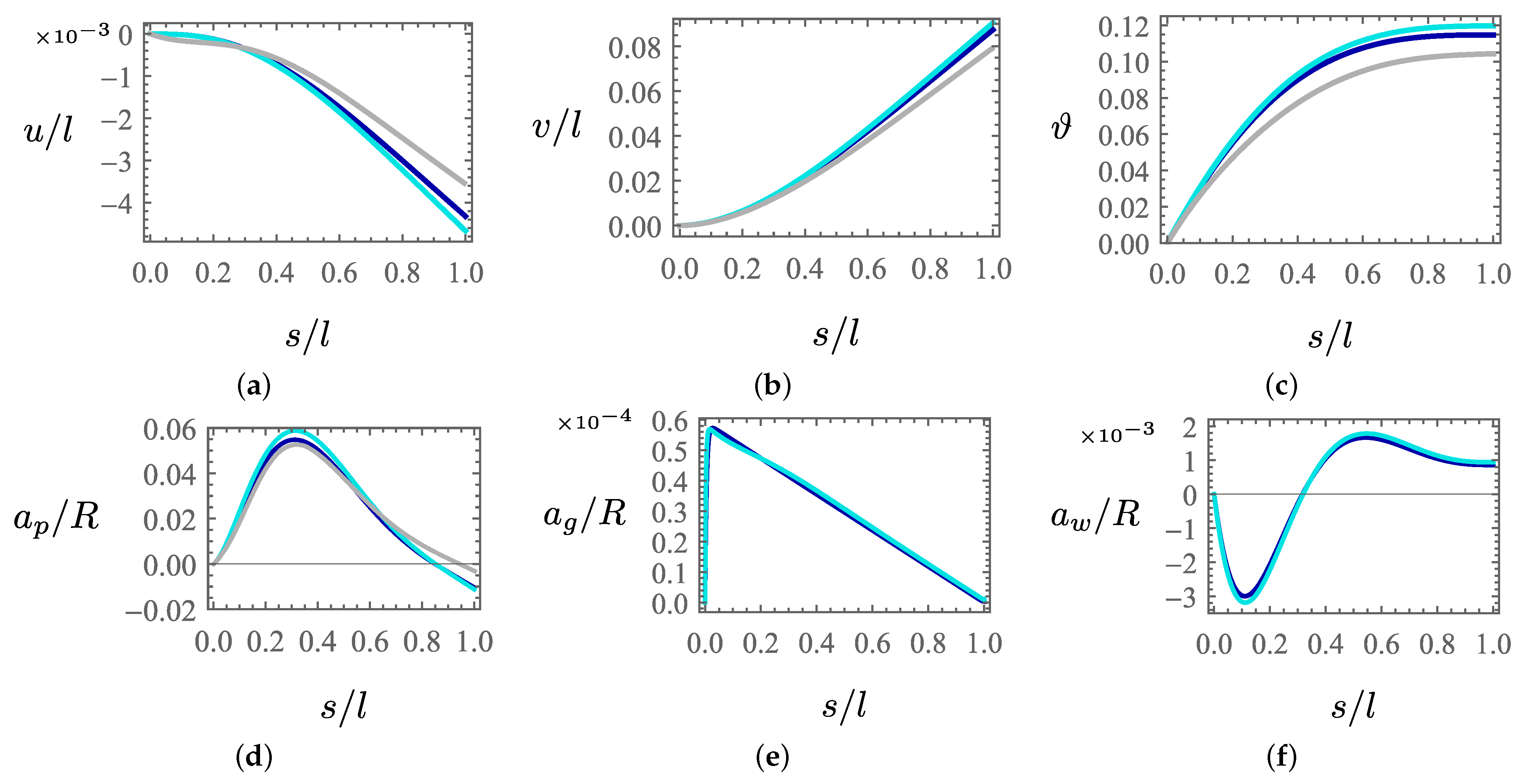
The outcomes for the first load case are shown as functions of $s/l$ in Figure 4, where (1) the perturbation solution is marked by the dark blue lines; (2) the numerical one obtained via the finite difference method is marked by light blue lines; and (3) that provided by the FEM model is marked by gray lines (note that variables $a_g$ and $a_w$ as given are not directly observable by the FEM model).

As expected, the effect of the distributed vertical load is evident on the variables v and $\vartheta$ (Figure 4b,c), which are directly activated at the linear order. However, due to the nonlinear coupling, the longitudinal displacement u is activated as well (Figure 4a), together with the local distortion variables (Figure 4d–f). In particular, the cross-section ovalization amplitude $a_p$ attains its maximum approximately at $s/l=0.35$, where the cross-section warping $a_w$ assumes zero value. Finally, the inter-layer sliding $a_g$, whose behavior is shown in Figure 4e, shows an almost linear behavior along the most part of the domain and a boundary layer close to the clamp (at $s=0$), where it suddenly goes to zero. It is remarked that the perturbation solution, with higher order corrections, well captures the response of the structure: marginal differences appear with the finite difference solution, since the curves are overlapped in the entire domain. Satisfying agreement is found in the comparison with the FEM solution, as well.

In Figure 5 the evolution of the displacement at the tip $v\left(l\right)/l$ (in abscissa) is shown when increasing the intensity of the load $\tilde{p}:=\frac{p_{v}l}{\pi R(G_e{h}_e+G_i{h}_i)}$ (in ordinate): the softening behavior due to the Brazier effect is well caught by the finite difference solution, and the perturbation solution correctly catches most of the curve except nearby the limit point. There, the agreement is less satisfying, perhaps due to the large distance of the limit point from the origin, and hence to the necessity of higher order approximation. The FE solution shows satisfying agreement as well, even if it is not very precise nearby the limit point, due to the approaching numerical instability. The dashed line in Figure 5 indicates the load condition corresponding to the previous Figure 4.

4.2. Concentrated Load

The response of the structure to the concentrated load $P_v$ at $s=l$ is now analyzed. The results are illustrated in Figure 6 in terms of the same quantities discussed in the previous case and the same color legend.

As observed before, the perturbation solution well approximates the one obtained via the finite difference approach and it is also in good agreement with the FEM solution. The applied load $P_v$ activates directly the variables v and $\vartheta$ (Figure 6b,c), which in turn activate the longitudinal displacement u (Figure 6a) and the local distortion variables (Figure 6d–f). In particular, the inter-layer sliding $a_g$ exhibits an almost constant evolution, except for the presence of the boundary layer at the clamp (Figure 6e); furthermore, for the same variable, the finite difference solution reveals a low amplitude oscillation around a mean value that is instead well captured by the perturbation solution.

In analogy with the distributed load case, in Figure 7 the evolution of the displacement at the tip $v\left(l\right)/l$ (in abscissa) is shown when increasing the intensity of the tip load $\tilde{P}:=\frac{P_v}{\pi R(G_e{h}_e+G_i{h}_i)}$ (in ordinate). The softening behavior is still more evident in the finite difference solution, even if both the perturbation and FEM solutions are in good agreement with it for most of the plot. The black dashed line still indicates the load condition corresponding to the previous Figure 6.

5. Conclusions

Nonlinear statics of a double-layered pipe under the action of transverse forces is addressed here through a perturbation method. The beam-like model, taken from the literature, provides nonlinear equilibrium equations in terms of kinematic descriptors, where those relevant to the classic Timoshenko beam are combined to further variables and introduced to account for local distortion. The perturbation scheme, tailored for the two loading conditions, which consist of distributed and tip forces, respectively, requires different scaling for the involved variables, in order to exploit their even or odd nature. The obtained closed-form solutions, evaluated up to the fourth perturbation order, guarantee very good agreement with those obtained via pure numeric tools, and concurrently, represent a valid tool to discuss the nature of the response, and potentially to optimize the choice of the relevant parameters.

In both the load conditions, the non-negligible contribution of the ovalization, which is directly coupled to the warping amplitude, appears as correctly determined by the asymptotic solution; the same happens for the small but significant effect of the longitudinal sliding, which shows a boundary layer close to the clamped cross-section. Moreover, the longitudinal displacement, which is triggered as a consequence of the nonlinear coupling, is non-negligible as well.

It is worth noting that in both the analyzed cases, good agreement of the outcomes provided by the perturbation method was obtained, even if the numerical values of the parameters slightly violated the hypotheses under which the scaling was chosen, being $E_e=10E_i$. This aspect represents a typical strength of the perturbation methods.

Moreover, the perturbation method also guides one to an enriching mechanical interpretation of the phenomena, as a consequence of the scaling proposed here, namely: (1) the external loads directly trigger the bending problem; (2) bending in turn induces ovalization, warping and axial displacement, as secondary and nonlinear effects; (3) the local distortion in turn gives high-order corrections to the leading global bending; (4) high-order correction to the local distortion is finally evaluated.

References

Reddy, J. An evaluation of equivalent-single-layer and layerwise theories of composite laminates. Compos. Struct.1993, 25, 21–35. [Google Scholar] [CrossRef]
Carrera, E. Theories and finite elements for multilayered, anisotropic, composite plates and shells. Arch. Comput. Methods Eng.2002, 9, 87–140. [Google Scholar] [CrossRef]
Timoshenko, S. History of Strength of Materials: With a Brief Account of the History of Theory of Elasticity and Theory of Structures; Dover: New York, NY, USA, 1983. [Google Scholar]
Hodges, D. Nonlinear Composite Beam Theory; American Institute of Aeronautics and Astronautics, Inc.: Reston, VA, USA, 2006. [Google Scholar]
Librescu, L.; Song, O. Thin-Walled Composite Beams. Theory and Applications; Springer: Dordrecht, The Netherlands, 2006. [Google Scholar]
Vlasov, V. Thin-Walled Elastic Beams; National Science Foundation and Department of Commerce: Washington, DC, USA, 1961.
Brazier, L. On the Flexure of Thin Cylindrical Shells and Other ’Thin’ Sections. Proc. R. Soc. Lond. A1927, 116, 104–114. [Google Scholar]
Luongo, A.; Zulli, D.; Scognamiglio, I. The Brazier effect for elastic pipe beams with foam cores. Thin Walled Struct.2018, 124, 72–80. [Google Scholar] [CrossRef]
Silvestre, N.; Camotim, D. Nonlinear Generalized Beam Theory for Cold-Formed Steel Members. Int. J. Struct. Stab. Dyn.2003, 3, 461–490. [Google Scholar] [CrossRef]
Ranzi, G.; Luongo, A. A new approach for thin-walled member analysis in the framework of GBT. Thin Walled Struct.2011, 49, 1404–1414. [Google Scholar] [CrossRef] [Green Version]
Piccardo, G.; Ranzi, G.; Luongo, A. A direct approach for the evaluation of the conventional modes within the GBT formulation. Thin Walled Struct.2014, 74, 133–145. [Google Scholar] [CrossRef]
Piccardo, G.; Ranzi, G.; Luongo, A. A complete dynamic approach to the Generalized Beam Theory cross-section analysis including extension and shear modes. Math. Mech. Solids2014, 19, 900–924. [Google Scholar] [CrossRef]
Latalski, J.; Zulli, D. Generalized Beam Theory for thin-walled beams with curvilinear open cross-sections. Appl. Sci.2020, 10, 7802. [Google Scholar] [CrossRef]
D’Annibale, F.; Ferretti, M.; Luongo, A. Shear-shear-torsional homogeneous beam models for nonlinear periodic beam-like structures. Eng. Struct.2019, 184, 115–133. [Google Scholar] [CrossRef]
Ferretti, M.; D’Annibale, F.; Luongo, A. Modeling beam-like planar structures by a one-dimensional continuum: An analytical-numerical method. J. Appl. Comput. Mech.2020. [Google Scholar] [CrossRef]
Luongo, A.; Zulli, D. Free and forced linear dynamics of a homogeneous model for beam-like structures. Meccanica2020, 55, 907–925. [Google Scholar] [CrossRef]
Zulli, D.; Luongo, A. Nonlinear dynamics and stability of a homogeneous model of tall buildings under resonant action. J. Appl. Comput. Mech.2020. [Google Scholar] [CrossRef]
Di Nino, S.; Luongo, A. Nonlinear aeroelastic behavior of a base-isolated beam under steady wind flow. Int. J. Non Linear Mech.2020, 119, 103340. [Google Scholar] [CrossRef]
Luongo, A.; Zulli, D. A non-linear one-dimensional model of cross-deformable tubular beam. Int. J. Non Linear Mech.2014, 66, 33–42. [Google Scholar] [CrossRef]
Zulli, D. A one-dimensional beam-like model for double-layered pipes. Int. J. Non Linear Mech.2019, 109, 50–62. [Google Scholar] [CrossRef]
Wolfram Research, I. Mathematica; Version 12.1; Wolfram Research, Inc.: Champaign, IL, USA, 2020. [Google Scholar]
COMSOL, I. COMSOL Multiphysics; COMSOL, Inc.: Stockholm, Sweden, 2015. [Google Scholar]
Figure 1.
The double-layered beam with an annular cross-section: (a) complete view; (b) details of the cross-section.
Figure 2.
Initial configuration of the beam.
Figure 3.
Physical meaning of the distortion variables: (a) assumed trial function for ovalization and amplitude ; (b) assumed trial function for warping and amplitude ; (c) assumed trial function for longitudinal sliding of the layers under opposite bending and amplitude .
Figure 4.
Response in the case of the uniformly distributed vertical load: (a) longitudinal displacement ; (b) ; (c) transversal displacement ; (d) amplitude of ovalization ; (e) amplitude of relative sliding ; (f) amplitude of warping . Blue lines: perturbation solution; light blue lines: finite difference method; gray lines: FEM.
Figure 5.
Distributed force: evolution of the tip displacements while increasing the amplitude of the load (). Black dashed line: load condition of Figure 4; blue line: perturbation solution; light blue line: finite difference method; gray line: FEM.
Figure 6.
Figure 7.
Tip force: evolution of the tip displacements while the increasing of the amplitude of the load (). Black dashed line: load condition of Figure 6; blue line: perturbation solution; light blue line: finite difference method; gray line: FEM.
Publisher’s Note: MDPI stays neutral with regard to jurisdictional claims in published maps and institutional affiliations.
Zulli, D.; Casalotti, A.; Luongo, A.