Article

Generalized Beam Theory for Thin-Walled Beams with Curvilinear Open Cross-Sections

by
Jarosław Latalski
1,† and
Daniele Zulli
2,*
1
Department of Applied Mechanics, Lublin University of Technology, 20-618 Lublin, Poland
2
Department of Civil, Construction-Architectural and Environmental Engineering, University of L’Aquila, Piazzale Pontieri, Loc. Monteluco, 67100 L’Aquila, Italy
*
Author to whom correspondence should be addressed.
Current address: 36 Nadbystrzycka Str., 20-618 Lublin, Poland.
Appl. Sci. 2020, 10(21), 7802; https://doi.org/10.3390/app10217802
Submission received: 16 September 2020 / Revised: 28 October 2020 / Accepted: 29 October 2020 / Published: 3 November 2020
(This article belongs to the Special Issue Homogenization Methods in Materials and Structures)

Abstract

:
The use of the Generalized Beam Theory (GBT) is extended to thin-walled beams with curvilinear cross-sections. After defining the kinematic features of the walls, where their curvature is consistently accounted for, the displacement of the points is assumed as linear combination of unknown amplitudes and pre-established trial functions. The latter, and specifically their in-plane components, are chosen as dynamic modes of a curved beam in the shape of the member cross-section. Moreover, the out-of-plane components come from the imposition of the Vlasov internal constraint of shear indeformable middle surface. For a case study of semi-annular cross-section, i.e., constant curvature, the modes are analytically evaluated and the procedure is implemented for two different load conditions. Outcomes are compared to those of a FEM model.

1. Introduction

Thin-walled beams are structural elements with three characteristic dimensions of different orders of magnitude: the thickness is small when compared to the dimensions of the cross-section, which in turn are small when compared to the beam length.
Starting from the second half of the 19th century, slender thin-walled members have found applications in civil and naval engineering as beams, columns, frame-works etc. Later they have been adopted to the needs of aeronautics and aerospace design, as well as, e.g., turbomachinery industry. They offer a number of advantages over the classical compact section beams. The most important ones are lightweight combined with strong rigidity and loads resistance, lower manufacturing costs due to reduced resource consumption and labor-saving design, lower transport and maintenance expenses etc.. Moreover, thanks to their specific layout they leave to the designer much more flexibility regarding the choice of the material and cross-section shape to meet any specific design requirements.
The slender thin-walled elements exhibit significantly different kinematic behavior when compared to solid section beams. In particular the profile warping occurs combined with elastic couplings involving bending and twisting; other local effects arise as well. Therefore, the recognized classical beam theories like Euler–Bernoulli and Timoshenko cannot be trustworthy to analyse thin-walled members.
The first successful attempt to model the kinematics of thin-walled beams was done by Vlasov [1]. He developed the Theory of Sectorial Area postulating the non-uniform torsion along the beam axis contributing to out-of-plane warping of the cross-section. This hypothesis was accompanied by further assumptions regarding the cross-section being rigid in its own plane and no shear deformability along the profile mid-line. Vlasov’s analytical model was widely adopted by the research community and extended over the years to account for other effects like geometric non-linearities in longitudinal deformations caused by large cross sectional rotation [2], shear deformability along the wall thickness [3], variable cross section specimens (stepped or tapered) [4,5], curved axis beams [6,7] or nonlinear warping effects [8].
A further generalization of Vlasov’s model was proposed by Capurso [9]. He revisited the original assumptions to include shear deformation over the cross-section midline by generalizing the description of warping. Later, significant research was focused on modern materials with directional properties like composites and laminates. The works by Librescu and Song [10] and Variational Asymptotic Beam Sectional (VABS) theory developed by Yu and Hodges [11] extending the original Vlasov model are particularly worth noting. Research on the dynamics of composite thin-walled beams with closed sections was also carried out by Latalski et al. [12,13].
According to the original assumptions on beam profile kinematics the Vlasov theory fails to take into account the effects of cross-section distortion and any local in-plane deformations of the walls. In this respect, The Generalized Beam Theory (GBT) is an alternative modeling concept that adds to the Vlasov’s model the distortion of the cross-section.
The method was originally developed by Schardt [14,15] to deal with buckling stability of prismatic cross-section columns. In its original formulation the slender thin-walled element was considered as an assembly of plate segments which are free to bend in the plane of the cross-section. The consequence of this assumption were in-plane deformations of the profile. The latter were assumed to be expressed as the superposition of a series of cross-sectional natural modes whose magnitudes varied along the member span. As a result the two-dimensional (2D) analysis within the shell framework theory is condensed into one-dimensional (1D) beam theory.
Since the mid 1990s, Schardt’s original theory received significant attention from the research community and was extended to take into account other cases and effects. Renton [16] proposed to use the Generalized Beam Theory to estimate the shear stiffnesses of various cross-sections as particular cases of a general analysis embracing torsion, bending, extension and shear of regular prismatic systems. Silvestre and Camotim [17] developed a geometrically nonlinear Generalized Beam Theory to consider large structural deformations. The proposed formulation was used to study the post-buckling behavior of steel columns with cold-formed thin-walled profiles. The presented analysis showed, among other things, the need to include shear and transverse extension modes to properly capture system kinematics. The relevant shear-deformable GBT structural model was elaborated and presented in authors later research [18,19]. Taig and Ranzi [20] adopted the GBT to study the response of prismatic thin-walled members stiffened at different cross-sections along their span.
Next, Ranzi and Luongo [21] revisited the standard GBT algorithm for the determination of the conventional modes, in which bending, shear and local modes are evaluated separately. Authors proposed to use the dynamic modes of an unconstrained planar frame similar in shape to the member profile to calculate cross-section in-plane deformation modes. Next, based on the enforcement of shear conditions, the out-of-plane warping component was evaluated.
Piccardo et al. [22,23,24] proposed the new method to evaluate a suitable basis of modes for the elastic analysis of thin-walled members. The suggested treatment relied on the solution of two distinct eigenvalue problems governing the in-plane and the out-of-plane free oscillations of a thin-walled beam cross-section. The first eigenvalue problem was solved posing an inextensibility condition for the planar frame beam having the shape of the TWB middle line. In the second eigenvalue analysis the transverse extension and membrane shear strain of the plate elements forming the cross-section were accounted for and modes orthogonal to the inextensional ones were calculated. The efficiency of the proposed method was confirmed by the outcomes of numerical examples.
The research was continued later by the authors to extend the theory to account for nonlinear effects exhibited by elastic thin-walled beams [25]. To this aim, both linear and nonlinear functions were used to describe the displacement field of the member cross-section. The admissible set of trial functions was determined requiring that the classic Vlasov’s kinematic hypotheses of the linear theory (i.e., (a) transverse inextensibility and (b) unshearability) were satisfied also in the nonlinear sense. An illustrative example of C-lipped cross-section beam with uniform thickness subjected to a uniform vertical pressure load was presented. The accuracy of GBT analytical results was confirmed by the outcomes of FE simulations.
Studying the invoked above references and other GBT related literature one observes the vast majority of research deals with polygon-like cross sections while the cases of non-prismatic open or closed profiles are very scarce. This results from the fact that curved geometries make the problem to find the cross-section deformation modes quite complex. The exception might be tubular beam designs studied by Schardt in [14], who presented solutions to the problem of uniform bending of a closed cylinder specimen. The analysis was enhanced by discussion of solution accuracy when approximating the cylinder profile by a regular polygon shape.
In recent years, Silvestre [26] investigated the buckling behavior of circular hollow section (CHS) members. He postulated to extend the cross section analysis and include axisymmetric and torsional modes apart from the set of classical orthogonal shell-type deformations of the profile. The presented discussion concerned the influence of member length on the critical stress magnitude and corresponding buckling mode shape. Comparison of the analytical GBT results to FE simulations by shell elements revealed very good consistency with respect to both local and global structural behavior. Afterwards, the author extended his research to account for elliptical cylindrical shells and tubes under compression [27]. The problem of variable curvature along the cross-section mid-line was solved by introducing parametric functions of tangential angle and their Fourier series expansions to approximate the local arch radius. The proposed formulation proved to be very effective since only three deformation modes (one local-shell, one distortional and one global) were required to accurately evaluate the buckling behavior of elliptical members for a wide range of specimen slenderness. The structural behavior of circular cross-section members was studied also by Nedelcu [28]. The author considered conical shells under three different boundary conditions and subjected to buckling load. In the proposed approach the member deformed configuration was approximated by a combination of the predetermined shell-type deformation modes.
Thereafter, Luongo and Zulli [29] adopted a GBT framework to analyse the ovalization of a tubular cross-section beam when subjected to bending. In the kinematic analysis of the member cross section, distortional and bi-distortional strains were introduced in addition to the regular strain measures of rigid cross-section beams. Several cases of static loadings applied at the free end were investigated followed by large-amplitude free vibrations analysis. This research was continued to account for tubular beams with a soft core, possibly made of foam materials [30]. The findings showed the inclusion of a foam core could improve performance of the pipes due to the shifted structural instability limit load. In the subsequent paper [31], Zulli adopted this model to capture the double-layered pipe designs. New terms representing longitudinal slipping of the two layers were added to the kinematic description of the structure profile. Next, a homogenization procedure was applied to obtain the nonlinear, coupled, elastic response function of the beam-like member.
An efficient method to model beams with arbitrary but open cross section shapes within Generalized Beam Theory was presented by Gonçalves and Camotim [32]. The core of this approach was a modified two-stage cross sectional analysis procedure. Within the first step the curved mid-line of the cross-section was finely approximated by a series of straight segments constituting the polyline. The second stage consisted in selection just a few of natural nodes of this polyline to generate the independent DOFs for warping analysis while the intermediate nodes of the profile were treated like in classic procedure. By this approach it was possible to describe the cross-section geometry accurately, without generating an excessive number of deformation modes. The method was applied to several cross-sections with curved walls and it was shown it assured sufficiently accurate results even with a rough selection of cross-section DOFs. The method proved to be particularly efficient for polygonal sections with rounded corners.
The presented above discussion and review of thin-walled structures bibliography demonstrates that the problem of structural behavior of thin-walled beams with curvilinear open profiles has not been comprehensively studied within the GBT framework. The main purpose of present contribution is to fill this gap and to derive the analytical model of a generic thin-walled curvilinear cross-sections beam within the GBT modelling framework. Therefore the outline of the paper is as follows. In Section 2.1 the analysis of the profile kinematics is presented and expressions for strains in curvilinear reference system are given. The constitutive law is introduced in Section 2.2, and the procedure for setting trial in-plane and out-of-plane warping functions is explained in Section 2.3. Next, in Section 2.4, the governing equations are derived by means of the Hamilton’s method. In 
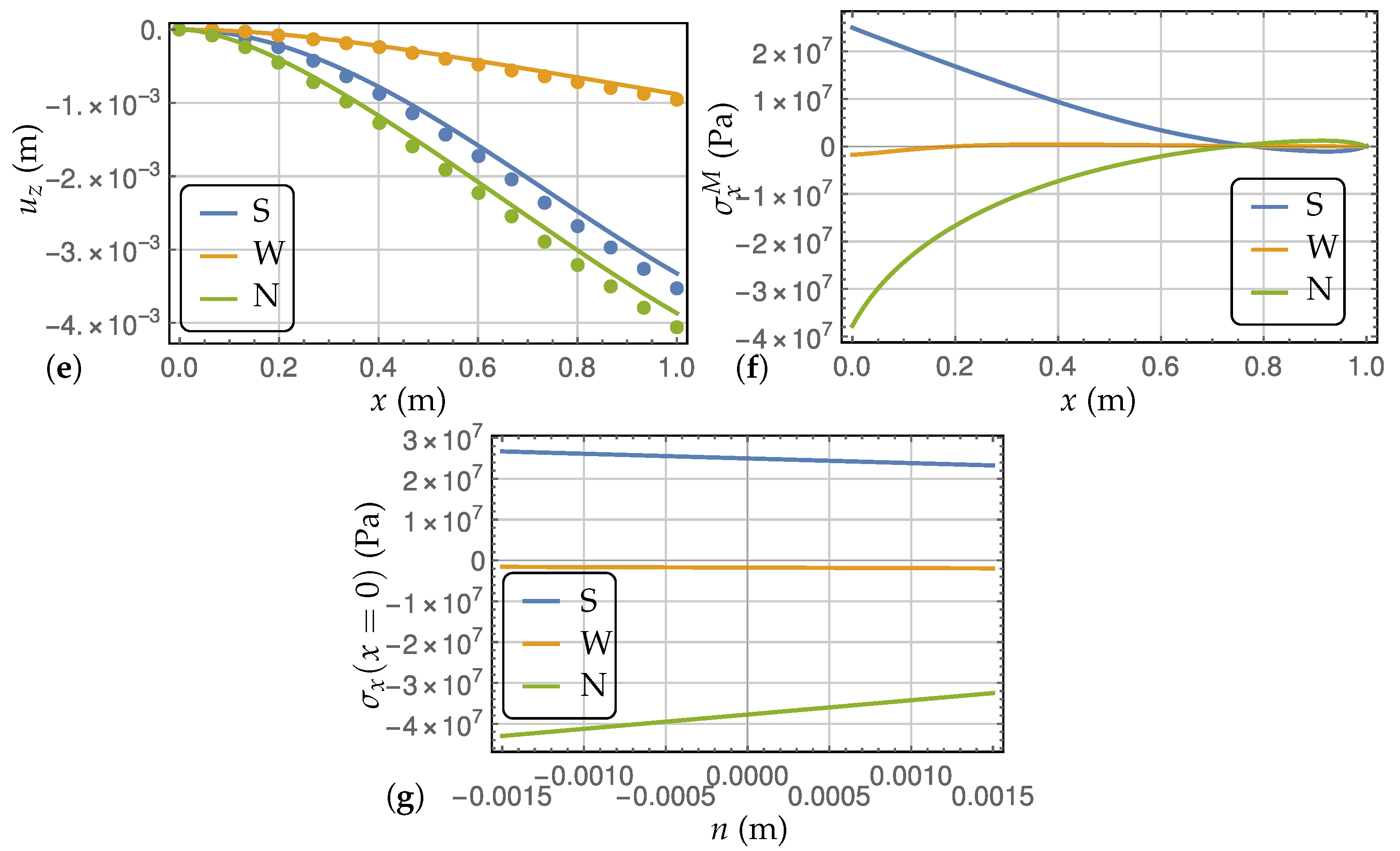
Section 3, the numerical examples of semi-annular specimen in two loading conditions are presented. The analytical results are compared to the outcomes of the FE simulations. Finally, the paper closes in Section 4 with the concluding remarks.

2. The Beam Model

A thin-walled beam made of isotropic, homogeneous and linearly elastic material is considered. The specimen is initially straight and its cross-sections, which are constituted by curved webs and flanges, are assumed open, while the closed and multi-cell cases are left for future developments. Furthermore, it is assumed that the profile of the beam is constant spanwise with no taper nor pretwist.
First, linear strain-displacement relationship is written and then, following the hypothesis of plane stress in profile walls, the constitutive law for linear elastic material is used to calculate strain energy. Finally, Hamilton’s principle is used and the equilibrium equations in terms of kinematic descriptors are obtained, imposing that the total potential energy attains a minimum in the class of compatible displacements. According to GBT framework, the displacements are considered as linear combinations of pre-established trial functions and kinematic descriptors which change along the axis line of the beam. The adopted cross-section modal shapes describe both rigid displacements, as in classical beam models, and changes in the shape of the profile characteristic for thin-walled members.

2.1. Geometry and Kinematics
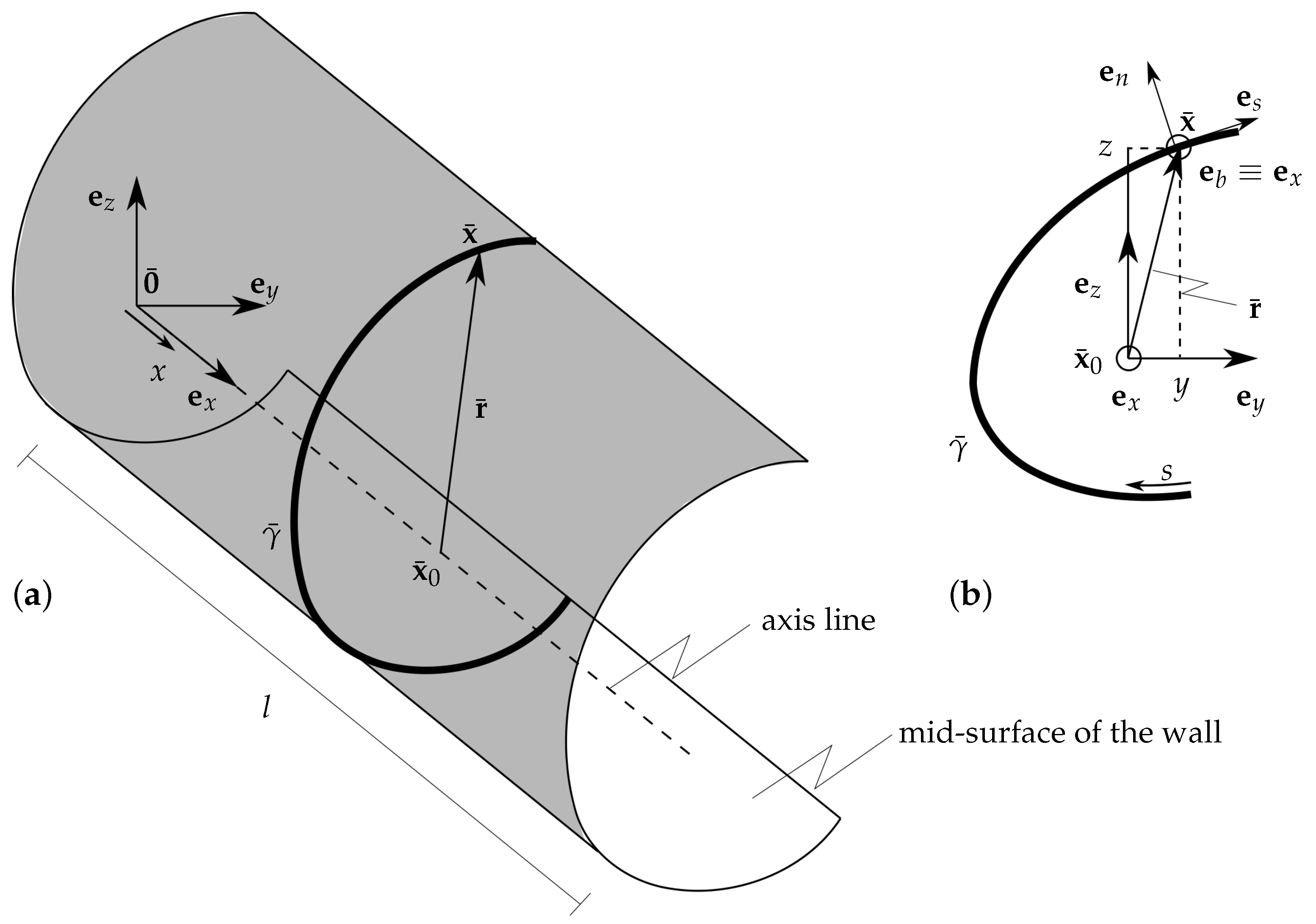
With reference to Figure 1, the axis line of the beam is defined in correspondence of the cross-sections centroids. It is a straight line given as:
x ¯ 0 ( x ) = 0 ¯ + x e x
where 0 ¯ is the position of the origin, which is the centre of the left tip cross-section, and x is an abscissa which runs in the interval [ 0 , l ] , where l is the length of the beam; the unit vectors ( e x , e y , e z ) are orthogonal to each other and define the canonical (global) basis. The initial position x ¯ of a generic point P located at the mid-surface of the wall is:
x ¯ ( x , s ) = x ¯ 0 ( x ) + r ¯ ( s )
where
r ¯ ( s ) = y ( s ) e y + z ( s ) e z
is the vector which defines the mid-curve γ ¯ of the cross-section, having curvilinear coordinate s as parameter. Specifically about the mid-curve γ ¯ of the cross-section, the parameter s is chosen so that d y d s 2 + d z d s 2 = 1 . Furthermore, it is convenient to set-up a local coordinate system along the curve and given by the tangent, normal and binormal unit vectors ( e s , e n , e b ) where—with respect to global basis—the relations follow:    
e s ( s ) = d y d s e y + d z d s e z e n ( s ) = d z d s e y + d y d s e z e b ( s ) = e x
and the curvature around e b is defined as:
k ¯ ( s ) = d y d s d 2 z d s 2 d z d s d 2 y d s 2
Through the beam deformation, the point P undergoes a displacement u , which can be expressed in terms of components on both the global and local bases, namely u x e x + u y e y + u z e z and u e s + v e n + w e b . According to Equation (4) the two sets of displacements are related as:
u = d y d s u y + d z d s u z v = d z d s u y + d y d s u z w = u x
In order to take into account the thickness h of the walls, the webs and flanges are considered as singly curved thin shells, whose mid-surface coincides with γ ¯ (Figure 2). The displacements of any generic point located off the mid-surface ( n 0 ) are obtained from the mid-surface counterpart ones using Kirchhoff’s thin plate assumption.
Thus, every line normal to the mid-surface at x ¯ before deformation remains normal after the deformation and relevant rotations about e s and e b directions are:
θ s = v x
θ b = v s + k ¯ u
respectively. It is worth noting how the second term in the right hand side of Equation (8) results from cross-section curvature about binormal axis [33].
As a consequence, any point out of the mid-surface performs displacement d which has the following components on ( e s , e n , e b ) :
d s = u n θ b d n = v d b = w + n θ s
respectively. Substituting Equations (7) and (8) into the above definitions, the local basis displacement components are as follows:
d s = u n v s + k ¯ u d n = v d b = w n v x
The infinitesimal strain components within the curved thin wall are defined as [33]:
ε x = d b x ε s = d s s k ¯ d n γ x s = d s x + d b s
where ε x , ε s are longitudinal strain along x , s , respectively, and  γ x s is the shear strain. After substituting Equation (10) in Equation (11), the strain components attain the following expressions:    
ε x = ε x M + ε x F ε s = ε s M + ε s F γ x s = γ x s M + γ x s F
where the pure membrane strain components, i.e., relevant to the mid-surface ( n = 0 ) and indicated with superscript M, and the flexural strain components, i.e., proportional to n and indicated with superscript F, are:
ε x M = w x ε s M = u s k ¯ v γ x s M = u x + w s
and
ε x F = n 2 v x 2 ε s F = n 2 v s 2 + k ¯ u s + k ¯ s u γ x s F = n 2 2 v x s + k ¯ u x
Following the idea of the Kantorovitch semi-variational method the individual components of the mid-curve γ ¯ points displacement are expressed as a linear combination of K triplets of trial functions ( U j ( s ) , V j ( s ) , W j ( s ) ) , j = 1 , , K , and unknown amplitude parameters a j ( x ) :
u ( s , x ) = j = 1 K U j ( s ) a j ( x ) v ( s , x ) = j = 1 K V j ( s ) a j ( x ) w ( s , x ) = j = 1 K W j ( s ) a j ( x )
where the prime indicates derivative with respect to x. The functions ( U j ( s ) , V j ( s ) , W j ( s ) ) represent the three components of the assumed j t h deformation field, defined on the section profile.
The use of Equation (15) in Equations (13) and (14) allows one to express the strain measures in terms of the kinematic descriptors a j ( x ) , for  j = 1 , , K :
ε x M = j = 1 K W j ( s ) a j ( x ) ε s M = j = 1 K d U j ( s ) d s k ¯ V j ( s ) a j ( x ) γ x s M = j = 1 K U j ( s ) + d W j ( s ) d s a j ( x )
and
ε x F = n j = 1 K V j ( s ) a j ( x ) ε s F = n j = 1 K d 2 V j ( s ) d s 2 + k ¯ d U j ( s ) d s + d k ¯ d s U j ( s ) a j ( x ) γ x s F = n j = 1 K 2 d V j ( s ) d s + k ¯ U j ( s ) a j ( x )

2.2. Constitutive Law

It is assumed that the beam is made of an isotropic, homogeneous and linearly elastic material. Moreover, the plane stress state hypothesis is adopted to a thin shell representing any individual beam wall. For thin-walled structures this assumption is realistic and provides reliable results. According to this formulation, the two-dimensional stresses are functions of solely two coordinates x and s, while all the transverse stresses are negligible:
σ n = τ s n = τ n x = 0
Thus, the corresponding 3D Hooke’s law is simplified to:
ϵ x = 1 E ( σ x ν σ s ) ϵ s = 1 E ( σ s ν σ x ) γ x s = τ x s G
where E , G , ν are the material Young’s and Kirchhoff’s moduli, and Poisson ratio, respectively. Equation (19), when solved in terms of stresses, becomes:
σ x = E 1 ν 2 ( ϵ x + ν ϵ s ) σ s = E 1 ν 2 ( ϵ s + ν ϵ x ) τ x s = G γ x s
Substituting Equation (12) in Equation (20), the expressions of the individual stress components can be decomposed to the sum of membrane and flexural related terms, as well:
σ x = σ x M + σ x F σ s = σ s M + σ s F τ x s = τ x s M + τ x s F
Finally, the use of Equations (16) and (17) allows one to express the stress components in (21) in terms of the trial functions ( U j ( s ) , V j ( s ) , W j ( s ) ) and kinematic descriptors a j ( x ) , j = 1 , , K . The final expressions are omitted for the sake of brevity.

2.3. Trial Functions and Vlasov’s Constraints

The regular Vlasov’s internal constraints specific for any open cross-section require that the profile mid-curve γ ¯ is inextensible and the middle surface of the thin-walled beam is shear indeformable. Thereby two relations follow:
ε s M = 0 γ x s M = 0
As a consequence, regarding Equation (16), every j-th set of assumed trial functions must satisfy the following conditions:
d U j ( s ) d s k ¯ ( s ) V j ( s ) = 0
U j ( s ) + d W j ( s ) d s = 0
In this study, the trial functions ( U j ( s ) , V j ( s ) , W j ( s ) ) , j = 1 , , K are evaluated in two stages as proposed by Ranzi and Luongo in [21]. At first, the in-plane deformation field components ( U j ( s ) , V j ( s ) ) are evaluated as the dynamical normal modes of the planar unconstrained inextensional (i.e., satisfying the first Vlasov’s condition) frame having the shape similar to profile mid-curve γ ¯ . Thereby the considered frame is constituted by a monodimensional curved beam element or assembly of them in case of piece-wise regularity of γ ¯ . Having found the in-plane deformation modes, at the next stage the third trial function W j ( s ) is determined. This represents the component relevant to the out-of-plane warping of the cross-section and it is consistently evaluated by integration of Equation (24). The emerging unknown integration constant is obtained by imposing the orthogonality condition of W j ( s ) to the uniform axial extension, i.e.,  γ ¯ W j ( s ) d s = 0 . Therefore, the triple of thus deduced deformation fields ( U j ( s ) , V j ( s ) , W j ( s ) ) satisfy both Vlasov’s conditions given by Equation (22).
In the above analysis a uniform mass per unit length is assigned to the referenced frame in order to evaluate the in-plane deformation components; the latter must also be consistent with Equation (23), i.e., the curved beam constituting γ ¯ is axially indeformable. Furthermore, a suitable normalization condition on the normal modes is imposed.
It is worth noting that, due to the lack of external constraints, among the set of determined in-plane modes, three independent rigid motions of the cross-section in its plane are present as well. These are two translations in directions e y and e z , respectively, and rotation about e x . Moreover, consistently with the internal constraint in Equation (24), the out-of-plane components relevant to the two translations in directions e y and e z turn out to describe rotations of the cross-section about axes e z and e y , respectively, as in an Euler–Bernoulli beam bending. Thus, it should be pointed out that, with the present approach, it is precluded the possibility of introducing independent bending rotations as it would be done in Timoshenko beam models.
An additional trial function, which describes the uniform extension in direction e x is defined as well, and it is assigned to ordering j = 1 . Therefore, the triplets ( U j ( s ) , V j ( s ) , W j ( s ) ) for j = 1 , , 4 describe rigid motions of the profile and are given as follows: j = 1 : ( 0 , 0 , 1 ) ; j = 2 : ( d y d s , d z d s , y ) ; j = 3 : ( d z d s , d y d s , z ) ; j = 4 : ( y d z d s z d y d s , y d y d s + z d z d s , ( y d z d s z d y d s ) d s + c 4 ) . The other triplets ( j > 4 ) describe in-plane deformation of the cross-section and its corresponding kinematically consistent out-of-plane warping.
It is worth mentioning that the Vlasov’s conditions (22) can be removed in the framework of GBT, as well: This is the case, for instance, of structures where shear-lag might occur, as shown in [22]; there, further trial functions are introduced, which account for both shear and extensional deformation.

2.4. Equilibrium Equations

Equilibrium equations in terms of generalized amplitudes a j ( x ) are obtained imposing the stationary condition to the sum of elastic and load potential energy (conservative external loads are assumed). In particular, the elastic potential energy has the following expression:
U e = 1 2 V σ x M ε x M + σ x F ε x F + σ s F ε s F + τ x s F γ x s F d V
where V is the total volume of the beam and the differential volume element being d V = d n d s d x . In the above the membrane components of strain in tangential direction s and shear mid-surface indeformability are omitted according to Vlasov’s conditions Equation (22).
After expressing the stress and strain components in Equation (25) in terms of the unknown amplitudes a j ( x ) , by means of the relevant equations from Section 2.1 and Section 2.2, the elastic potential energy becomes:
U e = 0 l 1 2 a · A a + a · B a + a · C a + a · F a d x
where a ( x ) : = ( a 1 ( x ) , , a K ( x ) ) T , the dot stands for scalar product, the prime indicates derivative with respect to x and the expressions of the elements of the individual matrices are:
A i , j = γ ¯ h 2 h 2 n 2 E 1 ν 2 d d s d V i d s + k U i d d s d V j d s + k U j d n d s B i , j = γ ¯ h 2 h 2 n 2 E 2 ( 1 + ν ) 2 d V i d s + k U i 2 d V j d s + k U j d n d s C i , j = γ ¯ h 2 h 2 E 1 ν 2 [ W i W j + n 2 V i V j ] d n d s F i , j = γ ¯ h 2 h 2 n 2 E ν ( 1 ν 2 ) d d s d V i d s + k U i V j d n d s
It is worth noting that A , B , C are symmetric matrices.
The load potential energy is evaluated for a general case of a force per unit area acting in correspondence of the mid-surface. The generally oriented force is defined by the three components vector p ( x , s ) = p x e x + p y e y + p z e z that yields the energy:
U l = 0 l γ ¯ [ p x u x + p y u y + p z u z ] d s d x
where the displacement components can be expressed in terms of a ( x ) as well, by means of Equations (6) and (15).
The minimum of the total potential energy is attained imposing that δ ( U e + U l ) = 0 , δ a j ( x ) , j = 1 , , K , where δ is the variation operator, which produces the following set of Euler-Lagrange equations:
C a + ( F + F T B ) a + A a = f
and boundary conditions in x = 0 , l :
a = 0 or C a + ( B F T ) a = g a = 0 or C a + F T a = 0
where the elements of f and g are:
f j = γ ¯ p y d y d s U j d z d s V j + p z d z d s U j + d y d s V j p x W j d s g j = [ γ ¯ p x W j d s ] x = 0 , l
Equations (29) and (30) represent a linear, ordinary differential boundary value problem with constant coefficients, governing the evolution of the functions a j ( x ) along the span of the beam. Even if it can be analytically solved using the well-known method of variation of constants, which provides the exact solution, numerical tools capable to solve BVP will be used to find the solution, for practical purposes. In spite of this, the outcomes will be referred to as analytical solution in the following part of the paper.
It is noteworthy that the case of branched cross-section can be addressed piecewise evaluating along γ ¯ the integrals in Equations (27) and (31).

3. Numerical Results

3.1. Definition of the Case-Studies

A thin-walled cantilever of length l = 1  m is considered for numerical analysis. The cross-section is semi-annular, with radius R = 0.1  m, uniform curvature k ¯ = 1 / R = 10 m 1 , and constant thickness of the wall h = 0.003  m (see Figure 3a). Defining the curvilinear abscissa s from the bottom end of the semi-annular, the curve γ ¯ turns out to be described by:
y ( s ) = 2 R π R   sin s R z ( s ) = R   cos s R
with s [ 0 , π R ] .
Two different load conditions are considered, namely load condition 1: p ( x , s ) = p e z in s [ π 2 R , π R ] (Figure 3a); load condition 2: p ( x , s ) = p e y in s [ 0 , π R ] (Figure 3b). In both cases p = 3 × 10 3 Pa. It is worth noting that the second load case respects full symmetry about the e y axis.
The material data used for the calculations correspond to the aluminium alloy having longitudinal elastic coefficient E = 84 GPa and Poisson ratio ν = 0.33 .

3.2. Trial Functions

With reference to Section 2.3, the in-plane trial functions ( U j ( s ) , V j ( s ) ) are analytically evaluated as the in-plane normal modes of a semi-annular inextensible Euler–Bernoulli beam matching the shape of the cantilever cross-section (Figure 3a), without any external constraints. Differently, in case of cross-sections with general expression of the curvature as a function of s, numerical techniques might be called for. Exclusively for this step, the mass per unit length m and the bending stiffness E I are assumed uniform and, conventionally, their values taken as m = 1 kg/m and E I = 1 Nm 2 . The normal modes of the arch beam turn out to be the solutions of the following eigenvalue problem (see [34]):
d U d s k ¯ V = 0
d V d s + k ¯ U Θ b = 0
k b = d Θ b d s
M = E I k b
d N d s k ¯ T + m λ U = 0
d T d s + k ¯ N + m λ V = 0
d M d s + T = 0
with natural boundary conditions in s = 0 , π R :
N = 0 T = 0 M = 0
where the above represent the normal and shear forces and bending moment, respectively.
In particular, Equation (33) states the vanishing of the axial strain of the arch beam, which corresponds to Vlasov’s condition of profile mid-plane inextensionality (see Equation (23) for comparison); Equation (34) states the vanishing of arch beam shear strain, where Θ b is the rotation of the cross-section of the arch about e b —this condition corresponds to former Kirchhoff’s assumption regarding wall bending. Equation (35) defines the bending curvature k b about e b , Equation (36) is the classical constitutive law for bending moment M and curvature k b , and Equations (37)–(39) are the balance equations for normal N and shear T forces, and bending moment M, respectively. The eigenvalue λ is the square of the circular frequency ω . It is worth noting that no constitutive law is used for N and T, they being the internal reactive forces to the constraints (33) and (34).
Assuming an exponential solution of type v ( s ) = v ^ e Ω s where v ( s ) = ( U , V , Θ b , k b , N , T , M ) T , after usual steps in modal analysis, the following bi-cubic dispersion equation is obtained:
E I Ω 6 + 2 E I k ¯ 2 Ω 4 + ( E I k ¯ 4 m λ ) Ω 2 + k ¯ 2 m λ = 0
Its roots Ω i ( λ ) , i = 1 , , 6 , after substitution in Equations (33)–(39), allow one to evaluate the relevant eigenvectors v ^ i and build the solution v ( s ) = i c i v ^ i e Ω i s , where c i are six undetermined constants. The latter expression is substituted in Equation (40) to get the first K natural frequencies (or λ ) and, for each of them, five of the six coefficients c i , while the sixth is given by the normalization condition.
As expected, λ = 0 is a solution of multiplicity 3, giving rise to three in-plane independent rigid motions. An additional rigid motion, required to describe the uniform displacement in direction e x , is prepended to them as reported at the end of Section 2.3.
Once the modal in-plane components U j ( s ) , V j ( s ) , j = 1 , , K are obtained, the out-of-plane ones W j ( s ) are evaluated as well, as  described in Section 2.3.
The first four modes, relevant to rigid motions, are shown in Figure 4 where, in the first and second row, the in-plane and out-of-plane components are drawn, respectively. In particular, in the first line, the in-plane components ( U j ( s ) , V j ( s ) ) are combined to show the actual displacement of the cross-section (in thick solid line), whereas, in the second row, the corresponding normal direction component W j ( s ) is plotted (as polar plot, still in thick solid line). Following the same rule, the first four in-plane deformation modes (i.e., which correspond to λ 0 ) are shown in the first row of Figure 5 and, in the second row, the corresponding out-of-plane components.

3.3. Equilibrium Configuration

Using the K = 8 trial functions discussed in Section 3.2, the equilibrium Equation (29) can be evaluated through Equation (27), and combined to the boundary conditions (30) relevant to the cantilever, i.e., geometric at x = 0 and natural at x = l . The obtained equations are then solved using a finite difference code based on the three-stage Lobatto IIIa formula, as implemented in the bvp4c library command in MATLAB [35], and the solution in terms of a j ( x ) , j = 1 , K , is used to calculate displacement and stress components in specific points of the thin-walled beam.
In particular, for the two load conditions, plots are shown for: kinematic descriptors a j ( x ) as functions of x [ 0 , l ] ; displacement components u x , u y , u z as functions of x for three points of the mid-curve γ ¯ , i.e., at positions where s = 0 (referred to as position S, i.e., the most southerly point), s = π R 2 (referred to as position W, i.e., the most westerly point), s = π R (referred to as position N, i.e., at the most northern point)—see also Figure A1 in Appendix A for reference; stress component σ x M as a function of x at the same three positions ( S , W , N ); stress component σ x as a function of n [ h 2 , h 2 ] at x = 0 in the same three positions. The GBT framework analytical solutions for u x , u y , u z are compared to the outcomes of a FEM model implemented in the Abaqus software (dotted lines in the plots). Details on the numerical model are given in Appendix A.
For the load condition 1 (load in e z direction), the solution is shown in Figure 6. From Figure 6a,b it can be observed that the component a 1 , corresponding to uniform extension, is always zero, as expected in a linear problem with structure subjected to transverse loads only. Moreover, amplitudes a j , j = 3 , , 6 have at least one order of magnitude larger than the remaining a 2 , a 7 , a 8 , revealing that global displacement along e y is almost zero and higher modes are actually not required for this case (it is verified, even if not reported here for the sake of brevity, that higher modes than K = 8 give vanishing contributions for the two analyzed cases). In particular, the components a 3 , a 4 , a 5 are those which give larger contributions, indicating that besides a rigid motion of the cross-section, a not-negligible deformation component related to a 5 (and in minor intensity a 6 ) is present.
In Figure 6c–e, the individual displacement components at the three points of the cross-section ( S , W , N ) are shown: the component u x comes only from warping of the cross-section and is much smaller than u z and u y . Significant in-plane rotation (about e x ) and change in shape of the cross-section are observed, as related to quite large a 4 and a 5 , respectively, as well as the expected slightly larger maximum displacement in direction e z (direction of the load). These outcomes reveal very good agreement with the FEM results. Consistently with Vlasov’s theory of non-uniform torsion [1], Figure 6f shows a change in sign of the axial stress component σ x M with respect to the contribution expected by simple bending: the latter is proportional to a 3 and would give negative value at S, zero value at W and positive value at N (Figure 4—component III-op); however, the change in sign is due to the large contribution of the out-of-plane distortion proportional to a 4 (Figure 4—component IV-op), whereas the non-zero value at position W is mainly due to the contribution of the out-of-plane distortion proportional to a 5 (Figure 5—component V-op). A not-negligible change in the values of σ x along the thickness of the cross-section is shown at positions N and S in Figure 6g, which contributes to the absolute value of the minimum and maximum stress, respectively.
For the load condition 2 (load in e y direction), due to the symmetry of the problem about axis e y , only modes respecting the same symmetry condition are used in the procedure, namely: II, V, VII in Figure 4 and Figure 5. The relevant amplitude components a 2 , a 5 , a 7 are shown in Figure 7a with clearly dominating role of the component a 2 corresponding to rigid motion of the cross-section. Furthermore, among them, a 7 is almost negligible as well. In Figure 7b,c, the symmetry of the problem causes the blue and green lines to be superimposed to each other, and satisfying agreement with FEM outcomes is noted. Distortion of the cross-section is evident, as confirmed by the displacement components u z in Figure 7d, which are opposite in sign for points S and N, respectively, as given by a 5 multiplying the V-ip trial function in Figure 5. Specifically for this displacement component, a non vanishing difference of GBT analytical and FEM numerical results is detected at the free tip relevant to positions N and S. The outcomes are anyway in very good agreement in most of the domain of the beam, i.e., for x [ 0 , 0.8 ] .
Figure 7e shows the axial stress component σ x M . The distribution is fully consistent with the contribution expected in simple bending test, with stress proportional to a 2 and multiplying the component II-op in Figure 4. Finally, a vanishing change in the value of resultant σ x along the thickness of the cross-section is shown at positions S and N in Figure 7f. This is due to the fact that the thickness of the profile wall in these points is perpendicular to the load direction thus the flexural component σ x F is immaterial.

4. Conclusions

A thin-walled beam with open and curved cross-section is considered in the paper, with the aim of formulating an analytical Generalized Beam Theory framework model for this specific case. Consistently, the displacements of the points of the walls are expressed as linear combinations of trial functions and unknown amplitudes. Then, by adopting the Hamilton’s principle, the equilibrium equations under external loads are evaluated taking into account the initial curvature of the members. As proposed in the literature [21], two components of trial functions are chosen as dynamical in-plane modes of the cross-section considered as a free beam. Consequently, the third out-of-plane component is evaluated imposing the validity of Vlasov’s internal constraint. Being the member cross-section in the shape of an arch, the trial functions are analytically evaluated solving the relevant eigenvalue problem, which provides both rigid (frequency zero) and deformation (frequency different than zero) motions. In case of elastic, isotropic and homogeneous material a case-study subjected to two load conditions is considered. The outcomes in terms of displacements are compared to those of a companion FEM model, showing generally good agreement. The provided results highlight the crucial contribution of the cross-section change in shape at equilibrium.

Author Contributions

Conceptualization, J.L. and D.Z.; Data curation, J.L. and D.Z.; Formal analysis, D.Z.; Investigation, J.L. and D.Z.; Methodology, J.L. and D.Z.; Validation, J.L.; Writing—original draft, J.L. and D.Z.; Writing—review & editing, J.L. and D.Z. All authors have read and agreed to the published version of the manuscript.

Funding

The research was financed in the framework of the project Regional Excellence Initiative funded by the Polish Ministry of Science and Higher Education (contract no. 030/RID/2018/19) and carried out at Lublin University of Technology.

Conflicts of Interest

The authors declare no conflict of interest.

Appendix A. FE Model

To verify the analytical results, the ABAQUS system finite element representation of the structure was developed. The beam under consideration was modelled by conventional linear quadrilateral shape shell elements with reduced integration (S4R). They are general-purpose elements capable to account for shear effects and provide correct results of displacements, strains, and stresses [36]. This type of elements is recommended for both thick and thin wall specimens approximating the Kirchhoff model as the thickness decreases. Moreover, this element accounts for finite membrane strains and arbitrary large rotations; therefore, it is suitable also for geometrically nonlinear analysis.
Alternatively, one can use continuum shell elements but they require the geometry to model explicitly the thickness of the shell, as it would be done with classical 3D solid elements. However, in contrast to the classical shell, continuum shell elements enforce the first order shear deformation constrains through particular element interpolation functions.
The beam structure was meshed into 100 elements along the span and 30 ones along the profile perimeter. Moreover, the nodal sets required to record the spanwise deflections at most southerly (S), most westerly (W) and most northern (N) positions of the profile were defined as shown in Figure A1.
Figure A1. Meshed FE model of the thin-walled cantilever and nodal points to record displacements.
Applsci 10 07802 g0a1

References

  1. Vlasov, V.Z. Thin-Walled Elastic Beams; National Technical Information Service: Jerusalem, Israel, 1961.
  2. Ghobarah, A.A.; Tso, W.K. A non-linear thin-walled beam theory. Int. J. Mech. Sci. 1971, 13, 1025–1038. [Google Scholar] [CrossRef]
  3. Simo, J.C.; Vu-Quoc, L. A geometrically-exact rod model incorporating shear and torsion-warping deformation. Int. J. Solids Struct. 1991, 27, 371–393. [Google Scholar] [CrossRef]
  4. Yang, Y.B.; Yau, J.D. Stability of beams with tapered I—Sections. J. Eng. Mech. 1987, 113, 1337–1357. [Google Scholar] [CrossRef]
  5. De Andrade, A.A.M. One-Dimensional Models for the Spatial Behaviour of Tapered Thin-Walled Bars with Open Cross-Sections: Static, Dynamic and Buckling Analyses. Ph.D. Thesis, University of Coimbra, Portugal, Coimbra, 2012. [Google Scholar]
  6. Yang, Y.B.; Kuo, S.R. Static stability of curved thin–walled beams. J. Eng. Mech. 1986, 112, 821–841. [Google Scholar] [CrossRef]
  7. Gendy, A.S.; Saleeb, A.F. Vibration analysis of coupled extensional/flexural/torsional modes of curved beams with arbitrary thin-walled sections. J. Sound Vib. 1994, 174, 261–274. [Google Scholar] [CrossRef]
  8. Di Egidio, A.; Luongo, A.; Vestroni, F. A non-linear model for the dynamics of open cross-section thin-walled beams—Part I: Formulation. Int. J. Non-Linear Mech. 2003, 38, 1067–1081. [Google Scholar] [CrossRef] [Green Version]
  9. Capurso, M. Influenza delle componenti di scorrimento nella deformazione delle travi di parete sottile con sezione aperta. G. Genio Civ. 1984, 122, 127–144. (In Italian) [Google Scholar]
  10. Librescu, L.; Song, O. Thin-Walled Composite Beams. Theory and Applications; Springer: Berlin/Heidelberg, Germany, 2006. [Google Scholar]
  11. Yu, W.; Hodges, D.H.; Volovoi, V.V.; Fuchs, E.D. A generalized Vlasov theory for composite beams. Thin-Walled Struct. 2005, 43, 1493–1511. [Google Scholar] [CrossRef]
  12. Latalski, J.; Warminski, J.; Rega, G. Bending-twisting vibrations of a rotating hub-thiun-walled composite beam system. Math. Mech. Solids 2017, 22, 1303–1325. [Google Scholar] [CrossRef]
  13. Latalski, J.; Warminski, J. Nonlinear vibrations of a rotating thin-walled composite piezo-beam with circumferentially uniform stiffness (CUS). Nonlinear Dyn. 2019, 98, 2509–2529. [Google Scholar] [CrossRef] [Green Version]
  14. Schardt, R. Verallgemeinerte Technische Biegetheorie: Lineare Probleme; Springer: Heidelberg, Germany, 1989. (In German) [Google Scholar]
  15. Schardt, R. Generalized Beam Theory—An adequate method for coupled stability problems. Thin-Walled Struct. 1994, 19, 161–180. [Google Scholar] [CrossRef]
  16. Renton, J.D. Generalized Beam Theory applied to shear stiffness. Int. J. Solids Struct. 1991, 27, 1955–1967. [Google Scholar] [CrossRef]
  17. Silvestre, N.; Camotim, D. Nonlinear Generalized Beam Theory for cold-formed steel members. Int. J. Struct. Stab. Dyn. 2003, 3, 461–490. [Google Scholar] [CrossRef]
  18. Silvestre, N.; Camotim, D. Influence of shear deformation on the local and global buckling behaviour of composite thin-walled members. In Thin-Walled Structures—Advances in Research, Design and Manufacturing Technology; Loughlan, J., Ed.; IOP Publishing Ltd.: Bristol, Italy, 2004; pp. 659–668. [Google Scholar]
  19. Silvestre, N.; Camotim, D. Shear deformable Generalized Beam Theory for the analysis of thin-walled composite members. J. Eng. Mech. 2013, 139, 1010–1024. [Google Scholar] [CrossRef]
  20. Taig, G.; Ranzi, G. Generalised Beam Theory (GBT) for stiffened sections. Int. J. Steel Struct. 2014, 14, 381–397. [Google Scholar] [CrossRef]
  21. Ranzi, G.; Luongo, A. A new approach for thin-walled member analysis in the framework of GBT. Thin-Walled Struct. 2011, 49, 1404–1414. [Google Scholar] [CrossRef] [Green Version]
  22. Piccardo, G.; Ranzi, G.; Luongo, A. A complete dynamic approach to the Generalized Beam Theory cross-section analysis including extension and shear modes. Math. Mech. Solids 2014, 19, 900–924. [Google Scholar] [CrossRef]
  23. Piccardo, G.; Ranzi, G.; Luongo, A. A direct approach for the evaluation of the conventional modes within the GBT formulation. Thin-Walled Struct. 2014, 74, 133–145. [Google Scholar] [CrossRef]
  24. Ferrarotti, A.; Piccardo, G.; Luongo, A. A novel straightforward dynamic approach for the evaluation of extensional modes within GBT ‘cross-section analysys’. Thin-Walled Struct. 2017, 114, 52–69. [Google Scholar] [CrossRef]
  25. Piccardo, G.; Ferrarotti, A.; Luongo, A. Nonlinear Generalized Beam Theory for open thin-walled members. Math. Mech. Solids 2016, 22, 1907–1921. [Google Scholar] [CrossRef]
  26. Silvestre, N. Generalised Beam Theory to analyse the buckling behaviour of circular cylindrical shells and tubes. Thin-Walled Struct. 2007, 45, 185–198. [Google Scholar] [CrossRef]
  27. Silvestre, N. Buckling behaviour of elliptical cylindrical shells and tubes under compression. Int. J. Solids Struct. 2008, 45, 4427–4447. [Google Scholar] [CrossRef] [Green Version]
  28. Nedelcu, M. GBT formulation to analyse the buckling behaviour of isotropic conical shells. Thin-Walled Struct. 2011, 49, 812–818. [Google Scholar] [CrossRef]
  29. Luongo, A.; Zulli, D. A non-linear one-dimensional model of cross-deformable tubular beam. Int. J. Non-Linear Mech. 2014, 66, 33–42. [Google Scholar] [CrossRef]
  30. Luongo, A.; Zulli, D.; Scognamiglio, I. The Brazier effect for elastic pipe beams with foam cores. Thin-Walled Struct. 2018, 124, 72–80. [Google Scholar] [CrossRef]
  31. Zulli, D. A one-dimensional beam-like model for double-layered pipes. Int. J. Non-Linear Mech. 2019, 109, 50–62. [Google Scholar] [CrossRef]
  32. Gonçalves, R.; Camotim, D. GBT deformation modes for curved thin-walled cross-sections based on a mid-line polygonal approximation. Thin-Walled Struct. 2016, 103, 231–243. [Google Scholar] [CrossRef]
  33. Axisa, F.; Trompette, P. Modelling of Mechanical Systems Vol 2 Structural Elements; Elsevier Butterworth-Heinemann: London, UK, 2005. [Google Scholar]
  34. Benedettini, F.; Alaggio, R.; Zulli, D. Nonlinear coupling and instability in the forced dynamics of a non-shallow arch: Theory and experiments. Nonlinear Dyn. 2012, 68, 505–517. [Google Scholar] [CrossRef]
  35. The MathWorks Inc. MATLAB; Version R2019b; The MathWorks Inc.: Natick, MA, USA, 2019. [Google Scholar]
  36. Smith, M. ABAQUS/CAE User’s Manual; Dassault Systèmes: Providence, RI, USA, 2020. [Google Scholar]
Figure 1. Thin-walled beam in initial configuration (a) and details of the mid-curve γ ¯ of the cross-section (b).
Applsci 10 07802 g001
Figure 2. Local sketch of the singly curved thin shell.
Applsci 10 07802 g002
Figure 3. Cross-section and load conditions in case-studies: (a) load condition 1; (b) load condition 2.
Applsci 10 07802 g003
Figure 4. In-plane (ip) and out-of-plane (op) components of the trial functions, from I to IV (rigid modes). Blue dashed line: initial configuration; black solid line: trial functions.
Applsci 10 07802 g004
Figure 5. In-plane (ip) and out-of-plane (op) components of the trial functions, from V to VIII (deformation modes). Blue dashed line: initial configuration; black solid line: trial functions.
Applsci 10 07802 g005
Figure 6. Solution for the load condition 1; S: s = 0 ; W: s = π R 2 ; N: s = π R ; (a) amplitudes a j , j = 1 , , 4 ; (b) amplitudes a j , j = 5 , , 8 ; (c) displacement u x ; (d) displacement u y ; (e) displacement u z ; (f) stress component σ x M ; (g) stress component σ x at x = 0 . Solid lines–analytical solution, dotted lines–FE solution.
Applsci 10 07802 g006aApplsci 10 07802 g006b
Figure 7. Solution for the load condition 2; S: s = 0 ; W: s = π R 2 ; N: s = π R ; (a) amplitudes a j , j = 2 , 5 , 7 ; (b) displacement u x ; (c) displacement u y ; (d) displacement u z ; (e) stress component σ x M ; (f) stress component σ x at x = 0 . Solid lines–analytical solution, dotted lines–FE solution.
Applsci 10 07802 g007aApplsci 10 07802 g007b
Publisher’s Note: MDPI stays neutral with regard to jurisdictional claims in published maps and institutional affiliations.

