Abstract
With the advancement of industrial intelligence, defect recognition has become an indispensable part of facilitating surface quality in the steel manufacturing process. To assure product quality, most previous studies were typically trained with many defect samples. Nonetheless, a large quantity of defect samples is difficult to obtain, owing to the rare occurrence of defects. In general, deep learning-based methods underperformed as they have inherent limitations due to inadequate information, thereby restraining the application of models. In this study, a two-level Gaussian pyramid is applied to decompose raw data into different resolution levels simultaneously filtering the noises to acquire compact and representative features. Subsequently, a multi-receptive field fusion-based network (MRFFN) is developed to learn the hierarchical features and synthesize the respective prediction scores to form the final recognition result. As a result, the proposed method is capable of exhibiting an outstanding performance of 99.75% when trained using a lightweight dataset. In addition, the experiments conducted using the disturbance defect dataset showed the robustness of the proposed MRFFN against common noises and motion blur.
1. Introduction
Towards smart factory for Industry 4.0, steel strip has become a ubiquitous material in most manufacturing workshops. In reality, owing to external factors such as equipment fatigue, human negligence, and external force, the steel surface may contain various types of defects. Consequently, these surface defects potentially affect the capability of steel products such as wear resistance, fatigue strength, and residual life [1,2], leading to huge economic losses for manufacturers and posing a high risk to worker safety. As such, defect recognition is an essential task for assuring product quality in manufacturing. Traditionally, defect inspection is performed manually by experienced laborers. However, this inspection task is time-consuming, inefficient, highly subjective, and unreliable under the heavy workload in the high-speed production line. Specifically, inspectors can only cover approximately 0.05% of total steel production [3], and the metal surface defects recognition rate is about 80%, despite most of them being trained professionally [4].
To overcome the shortcomings of human visual inspection, automated surface inspection (ASI) has drawn extensive attention from the computer vision community and the related research has grown rapidly in recent years. This paper attempts to tackle the surface defect inspection task on hot-rolled steel strips using a lightweight dataset. Succinctly, a two-level Gaussian pyramid with two multi-receptive field networks is introduced. Specifically, the Gaussian pyramid is applied to provide more meaningful samples for training models, at the same time suppressing the background noises from the raw images. Then, two pre-trained GoogLeNets [5] are fine-tuned separately, in which the shallower layers contain higher learning rate factors to improve the convergence speed of the model, while avoiding the training model falling into the local optimal situation. In addition, higher-level model is employed with fewer training parameters owing to the Gaussian pyramid process. Lastly, the prediction scores of both networks will be fused as the final prediction result. To further demonstrate the robustness of the proposed method, several experiments were carried out against Gaussian white noise, salt and pepper noise, and motion blur based on the disturbance defect dataset results. In brief, the main contributions of this work are summarized as follows:
- A multi-receptive field fusion-based network with a two-level Gaussian pyramid is introduced to extract more representative information from limited data.
- The shallower layers of the multi-receptive field fusion-based network (MRFFN) are applied with a higher learning rate to accelerate the convergence of the training process contemporary to avoid training models falling into the local optimal. Moreover, the higher-level model is fine-tuned with fewer training parameters to prevent the overfitting phenomenon, an inherent limitation.
- The proposed MRFFN achieves a pleasing performance compared with the state-of-the-art, which was trained by a relatively larger dataset. Furthermore, the MRFFN has shown its robustness against disturbance defect datasets, including Gaussian white noise, salt and pepper noise, and motion blur.
The remainder of the article is organized as follows. Section 2 reviews the related works based on defect recognition. Section 3 elaborates the details of the Gaussian pyramid and the proposed MRFFN. In Section 4, the evaluation of the proposed method will be presented. Section 5 reports and discusses the experimental results. Lastly, Section 6 concludes the article.
2. Related Work
2.1. Methods on Defect Recognition
Vision-based defect recognition can be loosely divided into designed-feature-based methods and learned-feature-based methods [6]. In particular, the former can be further separated into four types, statistical methods, filter-based methods, structural methods, and model-based methods, according to the defects texture [7]. Typically, most scholars indicated that the operator relied on the perception of the defects and achieved a pleasing performance. For example, Gan et al. [8] extracted the distribution features of leather defects, such as mean, variance, skewness, kurtosis, and lower and higher quartile values. The authors aimed to select the most suitable features and to eliminate the redundant information using the Kolmogorov–Smirnov test and percentile thresholding approach. However, the experimental results indicated that the above-mentioned methods are sensitive to imbalanced training data and the diversity of the defect area. Kumar et al. [9] applied a gray-level co-occurrence matrix (GLCM) to extract the defect features of welding and fed them into an artificial neural network (ANN) for classification. Wang et al. [10] proposed an optimal multi-feature-set fusion with an improved random forest algorithm (OMFF-RF), which applied GLCM and a histogram of oriented gradient (HOG) as the feature extractors. However, this method might be easily affected by background noises. Chondronasios et al. [11] utilized gradient-only co-occurrence matrices (GOCM) for extruded aluminum profiles classification.
On the other hand, Amid et al. [12] implemented a decision tree as the binary classification for defect and defect-free in the first stage, and introduced a multi-class SVM with an extended LBP-based operator to yield a sufficient performance in which the time consumed was acceptable for steel manufacturers. Liu et al. [13] improved the efficiency of the local binary pattern (LBP) algorithm by providing an improved multi-block local binary pattern algorithm. Besides, Yan et al. [14] applied a completed local ternary pattern (CLTP) as the feature extractor and adopted a binary-tree-based SVM as the classifier for weld defect detection. Succinctly, this method requires manual coordination for complicated weld images. On a similar note, Song et. al. [1] implemented an adjacent evaluation completed local binary pattern (AECLBP) to eliminate the interference of noise. Nevertheless, the experimental results showed that AECLBP is sensitive to Gaussian noise. To overcome the above-mentioned challenge, Chu et al. [15] proposed multi-type statistical features and enhanced twin support vector machines that are insensitive to affine transformation in scale and rotation. In a nutshell, most of the aforementioned approaches have a great influence on noise interference and affine transformation.
Thus far, plenty of works that adopted the concept of convolutional neural networks (CNNs) have been developed since the pioneering work carried out by LeCun [16] in 1998. Undoubtedly, learned-feature-based methods can describe the feature automatically with lower prior knowledge and achieve a breakthrough performance in most aspects. For instance, Masci et al. [17] used a Max-Pooling Convolutional Neural Networks for steel defect classification. Khumaidi et al. [18] applied CNN with the Gaussian kernel to eliminate noises from raw data. Besides, Lee et al. [19] proposed a VGG-like model with a class activation map to observe the explainability of the CNN and received an outstanding performance in steel surface defect tasks. In a similar fashion, Yang et al. [20] optimized the pre-trained VGG16 and visualized the intermediate activations of the CNN model. In addition, He et al. [21] introduced the classification priority network (CPN) with multi-group convolutional neural network (MG-CNN), which yielded promising results in hot-rolled steels. However, the above-discussed work requires a large number of training samples. Fu et al. [22] intended to improve the recognition results by fine-tuning the pre-trained SqueezeNet structure and adopted high learning rates for shallower layers so as to emphasize the low-level features. An analysis regarding the robustness of the proposed method used the addition of camera noise, non-uniform illumination, and motion blur. Furthermore, Chen et al. [23] trained three different deep CNNs and ensembled the prediction of the models to form the final result. The proposed methodology tended to prevail the state-of-the-art by yielding a near-perfect recognition rate. Nevertheless, the ensemble approach brought about a fatal weakness, viz., a large computational cost. In short, the above-mentioned approaches rely on plentiful training samples in which the defect data are inherently limited.
2.2. Autoencoder-Based-Methods for Light Defect Dataset
Toward the advancement of computational equipment, especially in the graphics processing unit (GPU), deep learning (DL) techniques have been widely adopted by researchers and received pleasing results for defect recognition tasks [24,25,26]. However, a large amount of training samples are unattainable in most situations, which will constitute the overfitting phenomenon during the deep model training process. Thereupon, autoencoder-based methods are proposed to overcome the shortcomings of DL techniques. Besides, He et al. [27] utilized a pre-trained Inception-V4 with a group of AutoEncoders to enhance the generalization of the model under inadequate training data. He et al. [28] applied a categorized deep convolutional generative adversarial network (cDCGAN) to generate mimic samples and cooperated with ResNet-18 to exploit unlabeled samples. Unfortunately, the limitation of autoencoder-based methods has been highlighted, where a massive amount of fake samples will exacerbate the misleading of DL models. In addition, Gao et al. [29] improved the CNN by integrating it with Pseudo-Label (namely PLCNN) to reduce the requirement for labeled training samples. On a similar note, Yun et al. [30] optimized the variational autoencoder (VAE) by a new convolutional VAE (CCVAE) to resolve the data imbalanced problem. Le et al. [31] adopted the Wasserstein generative adversarial nets (WGANs) for data augmentation and ensembled the pre-trained Inception and MobileNet to deal with the issues of imbalanced and small training data. Furthermore, Gao et al. [32] adopted a GAN-based DL method to reconstruct the defect images into higher-quality images to enhance the performance of the DL method. In short, the autoencoder-based methods can provide more vivid samples simultaneously for a denoising purpose. Yet, the elapsed time for generating fake images and the diversity of fake images should be determined in advance, otherwise it will bring counter-effect while training the model.
2.3. Deep-Learning-Based Methods for Light Defect Dataset
The inferior performance of DL-based methods under lightweight datasets has become a research hotspot in recent years. Although autoencoder-based methods can generate ample fake samples for the training model, the limitations of the above methods should also be considered. Briefly, the autoencoder-based methods still require a large number of training samples to form a pseudo-imagination, and the generated images should also be checked manually owing to the unstable training process which cannot facilitate the high-speed automated inspection tasks. In recent years, numerous pieces of literature have demonstrated the feasibility of DL-approaches in lightweight training sample tasks. For instance, Zhang et al. [33] froze the entire convolutional layers of the pre-trained VGG16 model and fine-tuned the fully connected layers with a new dense layer to reduce the computational load of the learning process. In this method, data augmentation techniques are applied to expand the training data and to simultaneously enhance the robustness of the model to the affine transformations. In addition, Tabernik et al. [34] designed a segmentation network to capture small defects and applied 1 × 1 kernel to the decision network as a channel reduction. The aforementioned study demonstrated a distinguished performance against the sensitivity to the number of training samples compared with the state-of-the-art segmentation networks. Feng et al. [35] attempted to reduce data dimensions and noise by applying principal component analysis (PCA), and adopted a deep neural network (DNN) to predict stainless steel defects. However, the results indicated that the PCA pre-processing led to nonlinear information losses, which had a deleterious influence on the training process. Furthermore, Ajmi et al. [36] implemented data augmentation techniques, simultaneously replacing the channel substitution with a Canny edge image and an Adaptive Gaussian thresholding image on the Weld X-ray image dataset. This method seems to provide a great improvement for providing more specific information to the training model. Additionally, Gao et al. [37] utilized a three-level Gaussian pyramid to provide multilevel information and adopted three VGG16 networks as the feature extractors. However, the experimental results demonstrated that the pre-trained model with lower trainable parameters yielded a better performance compared with the zero-fixed layers, which illustrates that the aforementioned method is prone to the overfitting phenomenon in the case of inadequate training samples. Similarly, the higher-level data contain relatively less information after applying several Gaussian pyramid processes. Thus, the overfitting problem will be exacerbated in the higher-level training model, which contains large-scale training parameters. To tackle this problem, Wan et al. [38] adopted a maximum and average feature extraction module, where they froze the first 15 layers of the pre-trained VGG19 to reduce the size of the training model.
3. Proposed Method
In this section, the principle of the Gaussian pyramid and the reason for selecting GoogLeNet as the backbone architecture will be explained. Furthermore, the multi-receptive field fusion-based network was proposed in which the models can learn different information from the small dataset.
3.1. Principle of Gaussian Pyramid
In light of the fact that data collection is limited, it is hard to assemble ample training samples for the large-scale network. A classical decomposition method known as the Gaussian pyramid [39] is exploited herein. The Gaussian pyramid decomposes the input data into a lower dimensionality contemporary, suppressing the redundant noise from the raw data. Specifically, assuming that the input image has a dimension of M × N, the original image is convolved by the Gaussian kernel and is downsampled into lower-dimensional images. The arbitrary pixel at spatial location (i, j) can be determined as follows:
where 0 ≤ i ≤ , 0 ≤ j ≤ is the size of the downsampled image, and w(u, v) represents the Gaussian window, which can be obtained by the following equation:
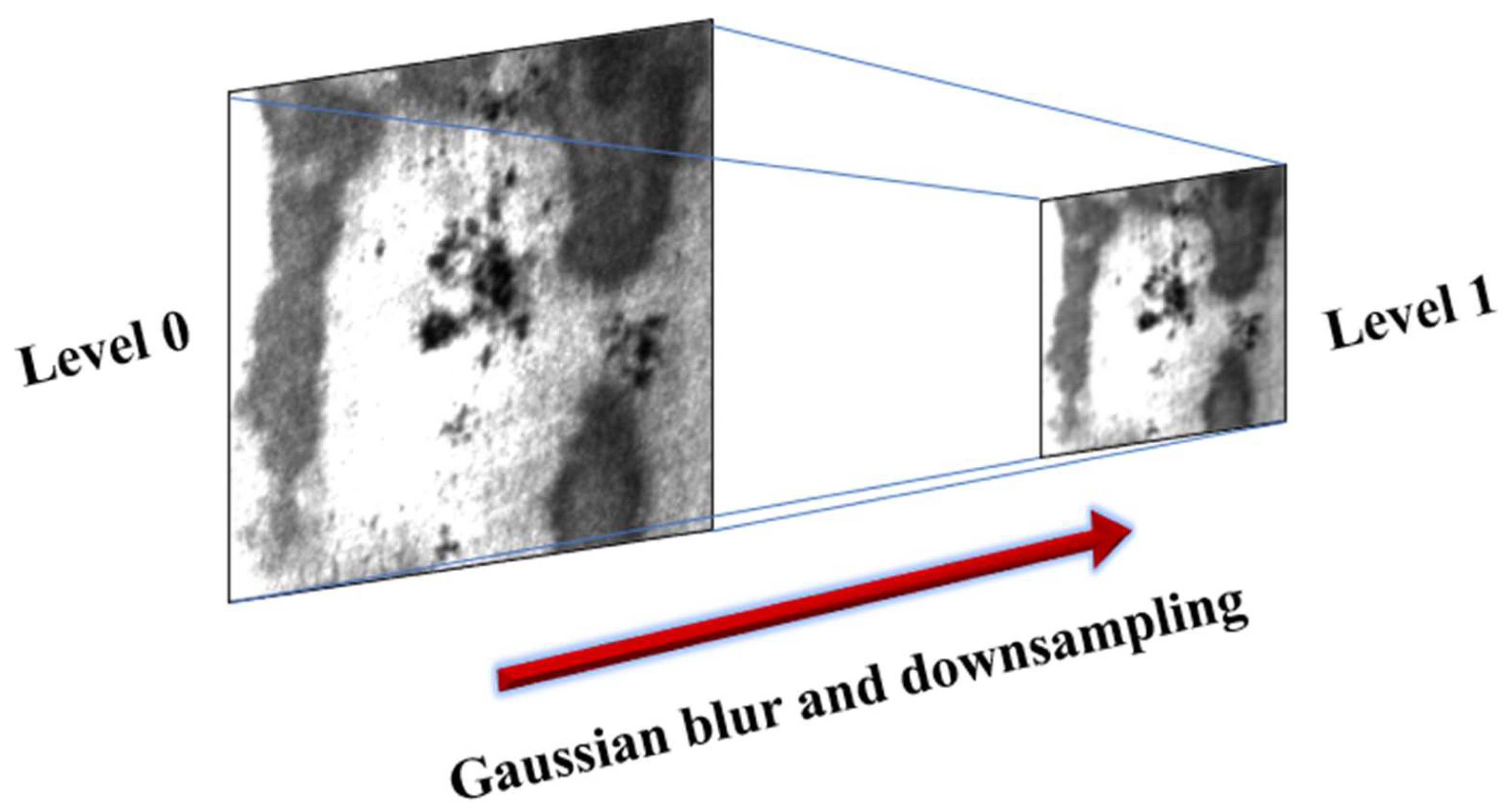
where parameter refers to variance. Here, the Gaussian kernel is applied as 5 × 5 to provide global information simultaneously and to retain important details for the training model. Multiple low-pass filters are applied to extract discriminant features from high-dimensional data and provide multiscale sub-images {, , , …, } for the training model, where 1, 2, 3,..., n represent the levels of the Gaussian pyramid. Here, a two-level Gaussian pyramid is utilized to decompose the source dataset into two different resolution sub-images, as shown in Figure 1, and the reason behind the application of a two-level Gaussian pyramid will be discussed in Section 5.1.
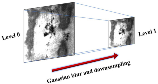
Figure 1.
The results of the Gaussian pyramid. Level 0 represents the raw image and level 1 represent the downsampled image, which contains only half of the level 0 resolution.
3.2. GoogLeNet-based Defect Recognition
So far, numerous novel works have attempted to utilize the deep CNN model to better characterize the complex defect features [23,37,40], and they yielded a favorable performance on surface defect inspection. However, these deep CNN models include tons of weights and biases that impair the efficiency of DL approaches, as well as inadequate training datasets. To take advantage of deep CNN contemporary and to address the drawback of increasing the network depth, GoogLeNet was introduced by Christian Szegedy [5] in 2015. Unlike most other deep networks, GoogLeNet implements a series of inception modules in which the 1 × 1, 3 × 3, and 5 × 5 convolutional layers are layered to each other to extract multiscale discriminative features. Meanwhile, to prevent the computational blow-up, 1 × 1 convolution layers are employed as a bottleneck before proceeding 3 × 3 and 5 × 5 convolutions, as shown in Figure 2. Recently, GoogLeNet has been widely adopted in various aspects and has exhibited a breakthrough recognition performance [41,42]. In this respect, GoogLeNet seems to have a deeper, yet lighter structure in comparison with AlexNet [43] and VGG-Net [44], which contain 6.8 million training parameters.
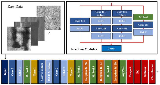
Figure 2.
The architecture of the pre-trained GoogLeNet. Conv represents the convolutional layer, M. Pool represents the max pooling layer, Norm represents the local response normalization, and Avg Pool represents the average pooling.
Additionally, the complex circumstances of the hot-rolled plates bring about an overwhelming challenge to surface defect recognition. For instance, local anomalies such as inclusion, patches, and scratches exhibit large spots or stripes, which are more conspicuous in comparison with global defects. On the contrary, global defects such as pitted surface, crazing, and rolled-in scale appear in a scattered manner in the form of speckles, bumps, or cracks, which are highly difficult to detect with the model. In brief, the large diversity of the surface defect appearance tends to be a great challenge for the feature extraction process. Thus, this study adopted pre-trained GoogLeNet as the backbone architecture to deal with the issues of limited data and large appearance diversity. Concisely, the details of the pre-trained GoogLeNet structure are shown in Table 1.

Table 1.
The details of the pre-trained GoogLeNet structure.
3.3. Multi-Receptive Field Fusion-Based Network (MRFFN)
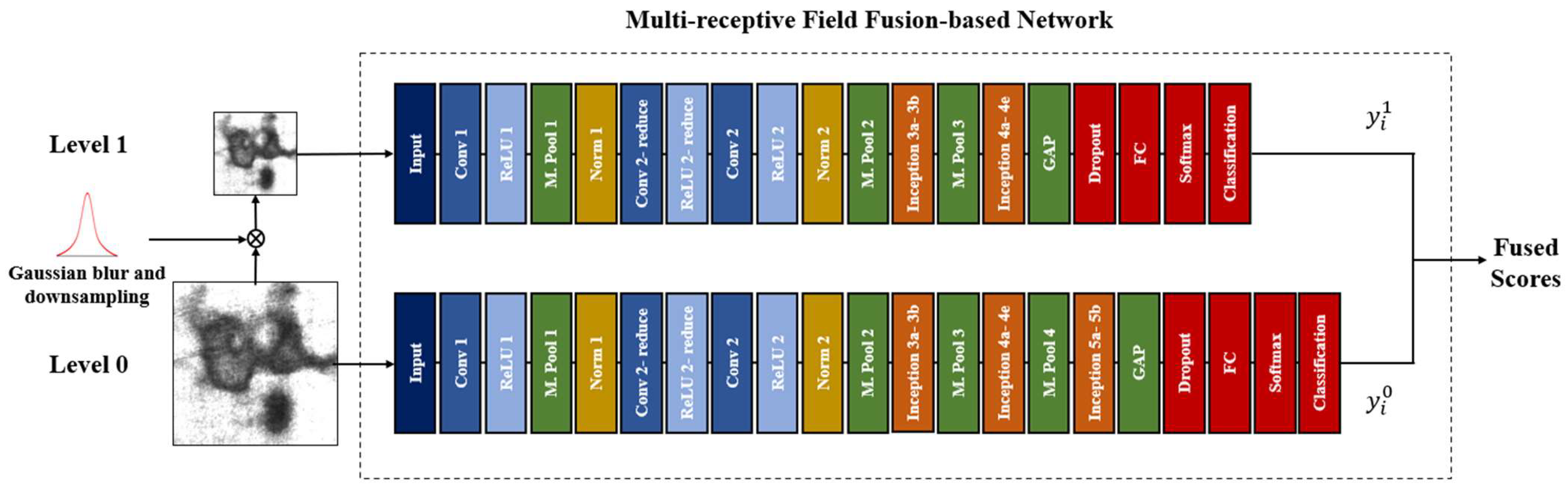
As it is difficult to collect sufficient defect samples for the deep network, the main challenge in this study is to extract more significant features from limited data. Concretely, two pre-trained GoogLeNets are adopted as the backbone architecture of the MRFFN. Here, the input size of the level 0 model is modified to 200 × 200, which contains the exact same resolution as the input images. Thereafter, the Gaussian pyramid downsamples the original images into a spatial resolution of 100 × 100 pixels, providing less information for the training model. This, however, appears to be inadequate for the deep structure like GoogLeNet to tackle the lower resolution images. Thus, the input size of the level 1 model is set to 100 × 100 pixels to prevent the risk of an overfitting phenomenon. Besides, the last two inception modules (i.e., inception module 5a and inception module 5b) of the pre-trained GoogLeNet have been discarded to scale down the computational load of the level 1 model. The overall framework of the proposed method is shown in Figure 3.

Figure 3.
The overall framework of the proposed method. First, the original images are decomposed by the Gaussian pyramid. Then, level 0 and level 1 are trained individually by the low-level and high-level images. Lastly, the confidence scores of both networks are fused to obtain the final result.
Succinctly, the GoogLeNet was pre-trained with 1.2 million samples from 1000 categories (e.g., animal, flower, tool, building, and fruit) and thus equipped with optimal weights for the classification task. However, the target object herein is steel surface defects, which have a large discrepancy to that of pre-trained samples. Hence, to better characterize the pattern of the steel surface defects, the shallower layers of both the level 0 and level 1 models are adopted with higher learning rate factors. Here, the learning rate factors of the Conv 1, Conv 2-reduce, Conv 2, inception module 3a, inception module 3b, and inception module 4a are applied as 9, while the other layers remain the same. By increasing the learning rate factors of the shallower layers, the convergence speed of the training models can be improved while reducing the gradient vanishing problem. Furthermore, the average pooling of both models is replaced with the global average pooling (GAP) to extract the global information of each feature map. Meanwhile, the fully connected layer of the original network is replaced with a new fully connected layer that has the same output as the NEU dataset classes. Lastly, the final prediction scores can be derived by fusing both the level 0 and level 1 network prediction results using the equation below:
where and indicate the highest and the second-highest predictions scores on the arbitrary testing image, and and indicate the probabilities of the class i defect according to level 0 and level 1 models, respectively. In order to avoid contains two highest prediction scores, the weights of level 0 and level 1 models are set as 0.6 and 0.4, while and are the same, and the explanation will be shown in Section 5.2.
4. Experimental Results
This section will introduce the experiment environment including the dataset description, hyperparameters, and the comparison of the result based on the NEU dataset and disturbance defect dataset.
4.1. Implementation Details
All of the experiments were carried out on MATLAB R2021a in Intel Core i7-10700F 2.90 GHz processor, RAM 64.0 GB, GPU NVIDIA RTX 3090. In this experiment, 50 images of each defect were randomly selected as the training data, and the remaining images served as the testing data. Notice that the image augmentation (IA) techniques were adopted herein to improve the performance of the proposed method under data-limited scenarios. Based on some experimental results, image reflection operation was heuristically selected only as the image augmentation technique to improve the training progress. Specifically, the training samples were randomly reflected horizontally or vertically with 50% probability. The models were trained for 300 epochs with an initial learning rate of 0.0001, and the mini-batch sizes were set as 300. All of the experiments were optimized by the Adam [45] algorithm and were repeated ten times to obtain reliable results.
4.2. Datasets Analysis
In this study, a typical steel surface defect dataset, namely Northeastern University (NEU) dataset [1], was utilized to evaluate the performance of the proposed method. The NEU dataset consists of six typical surface defects, viz., crazing (Cr), inclusion (In), patches, (Pa), pitted surface (PS), rolled-in scale (RS), and scratches (Sc). In total, the NEU dataset contains 1800 grayscale images with a spatial resolution of 200 × 200 pixels, and approximately 300 defect images were collected in each class. The examples of the NEU dataset are shown in Figure 4. From these examples, it can be seen that the complex variance of the surface defects and the influence of the illumination are challenging issues for describing the dataset.
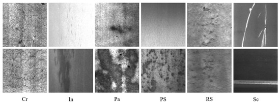
Figure 4.
The examples of the NEU dataset, where Cr, In, Pa, PS, RS, and Sc denote the crazing, inclusion, patches, pitted surface, rolled-in scale, and scratches defects, respectively.
To illustrate the complex variance of defects, Hao et al. [2] demonstrated the ratio distribution and size distribution of steel surface defects based on the NEU-DET dataset. Intuitively, up to about three-quarters of the surface defects were measured to have a ratio of the long side to the short side between one to three. Meanwhile, most of the surface defects were small in scale according to the distribution of the ratio of the defect area to the image area. In short, these results indicated that the inter-class defects had a limited diverse appearance. Besides, defects such as pitted surface, inclusion, and scratches contain large differences in appearance. For instance, according to Figure 4, it is obvious that the inclusion and pitted surface defects contained noticeable changes in their size and grayscale. Moreover, the appearance of the scratches defect might be horizontal, vertical, or slanting stripes. Hence, the intra-class diversity and inter-class similarity might exacerbate the misleading of the training model.
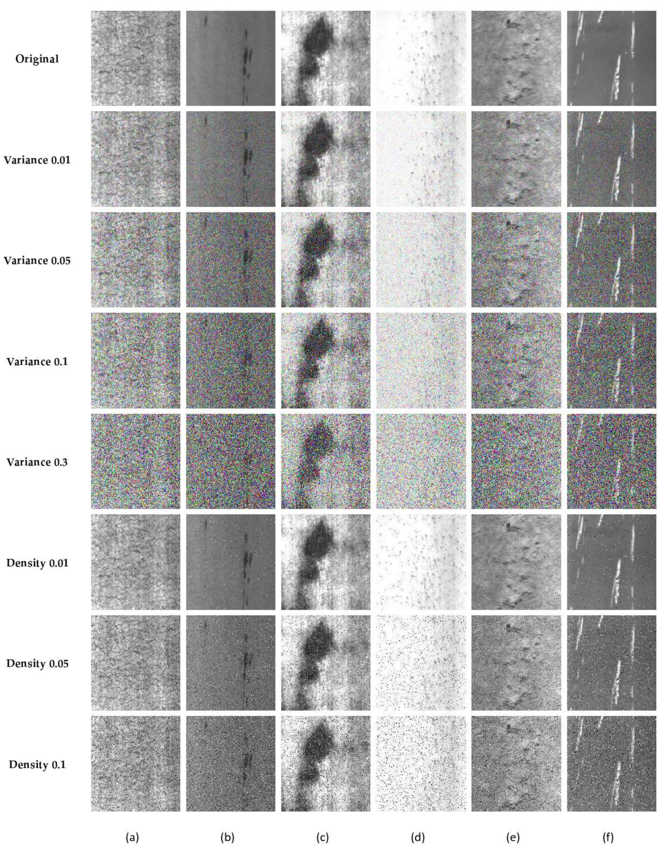
Furthermore, the disturbance defect dataset is constructed herein to evaluate the robustness of the MRFFN. The interference defect dataset involves two common noises in the actual production environment, which are Gaussian white noise and salt and pepper noise. According to Luo et al. [46], due to the high temperature of the image sensor or the lack of illuminance, the occurrence of Gaussian noise will occur during data collection. Besides, the transmission error by the camera will generate random black or white points (salt and pepper noise) and disturb the feature learning progress. Moreover, the high speed of the production line should be considered as it may cause a motion blur effect while capturing images. Hence, this study provides three common interference situations in the image acquisition process, including Gaussian white noise, salt and pepper noise, and motion blur. First, the variance of the zero-mean Gaussian white noise is set as 0.01, 0.05, 0.1, and 0.5 accordingly. Second, the density of salt and pepper noise is set as 0.01, 0.05, 0.1, and 0.5. Lastly, the length of the motion is set as 5, 10, 15, and 20 with a stochastic angle between 0° and 360°, as shown in Figure 5. For the interference defect dataset, 50 samples for each type of defect are randomly picked as the training samples and the remaining samples are regarded as the testing samples.
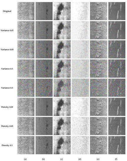
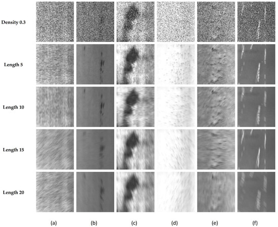
Figure 5.
The examples of the disturbance defect dataset. (a) Crazing, (b) Inclusion, (c) Patches, (d) Pitted Surface, (e) Rolled-in Scale (f) Scratches.
4.3. Parametric Measures
In this section, four indicators will be introduced to evaluate the performance of the experimental results. These indicators include the accuracy, recall, precision, and F1-score and are often used for measuring classification tasks, and can be mathematically defined as follows:
where TP, TN, FP, and FN denote the true positive, true negative, false positive, and false negative, respectively. Accuracy can be regarded as the rate of correct prediction among all of the tested samples. Recall can be defined as the correct prediction rate of positive samples among the labelled positive samples, and precision is the correct prediction rate of the true positive samples among the predicted positive samples. Furthermore, the F1-score is reported herein to harmonize the performance between recall and precision, where value of 1 indicates highest performance and the worst score is 0.
4.4. Comparison with State-of-the-Art Based on NEU Dataset
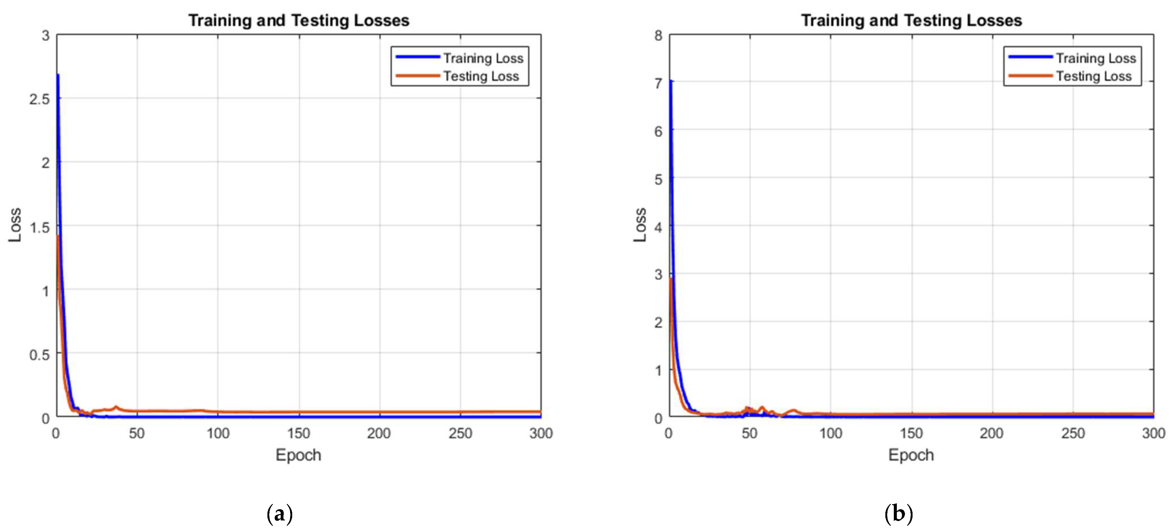
Figure 6 shows the training and testing losses of the level 0 and level 1 models. It can be seen that both networks have a high convergence speed in the first 100 epochs. While comparing the training progress between the level 0 and level 1 models, the testing loss of the level 0 model is much closer to the training loss. This result indicates that the level 1 model contains a higher risk of the overfitting phenomenon owing to less information being provided for the training model. Lastly, the testing loss gradually stabilized after training for 100 epochs, and the experimental results indicate that the testing loss almost remained the same during 200 to 300 epochs. Hence, this result suggests that 300 epochs are suitable for training the models.

Figure 6.
The training and testing losses of the models. (a) Training progress of the level 0 model and (b) training progress of the level 1 model.
Furthermore, this section compares the effectiveness of the proposed MRFFN with the state-of-the-art, which includes the ML-based, conventional CNN, and the fusion-based method. In particular, these methods were trained by a relatively larger dataset to better illustrate the performance of the MRFFN under data-limited tasks, and the table of comparison is shown in Table 2. Obviously, the low-level and high-level models obtained different performances, in which the low-level model was 0.27% higher than the high-level model. This result indicates that some representative information was eliminated while applying the Gaussian filter. Thus, the limitation of the Gaussian pyramid should be considered in order to prevent the deterioration of the training progress with limited data. Furthermore, the level 0 model tends to prevail over methods trained by 50 or 150 samples/defect [1,24,37,47]. This result indicates that the fine-tuned structure could better learn the meaningful features from the raw data. Furthermore, the results of the MRFFN shows that the combination of the level 0 and level 1 models can improve the performance of the models. The accuracy of MRFFN is 0.31% higher than the level 0 model and is 0.58% higher than the level 1 model. This shows that both networks are complementary to each other. This result also reveals that the proposed MRFFN yielded the best performance compared with the state-of-the-art [1,19,24,37,47]. Thus, it is convincing to state that the proposed method is able to generate more meaningful information from the raw data contemporary and to extract the important features effectively. Lastly, the performance of MRFFN increased by 0.14% when applying the image augmentation technique.
Table 2.
Comparison of results with the state-of-the-art based on the NEU dataset (%).
To investigate the classification results of the proposed MRFFN among six kinds of defects, the confusion matrix is provided in Table 3. From the confusion matrix, the first row represents the ground truth of the defect category, and the value in each column indicates the prediction results of the proposed method. According to the confusion matrix, the proposed MRFFN can easily recognize the patches defect, which yields a perfect precision and recall result. Besides, the MRFFN has achieved high recall (100%, 99.6%, and 100%) among crazing, pitted surface, and rolled-in scale, which is challenging to detect. However, the result demonstrates that the MRFFN gets confused by the inclusion and pitted surface defects, in which 0.72% of inclusion samples are misclassified as the pitted surface, and 0.20% of the pitted surface samples are misclassified as inclusion.
Table 3.
The confusion matrix of MRFFN + IA based on the NEU dataset (%).
4.5. Performance on Disturbance Defect Dataset
4.5.1. Recognition Results on the Disturbance Defect Dataset
In the real-world manufacturing process, the images captured may not be the same as in the public dataset. For example, low luminance, different viewpoint problems, and inevitable factors (i.e., vibration and white noise) will directly influence the quality of the images. To further evaluate the robustness of the proposed MRFFN, the disturbance defect dataset is utilized in this experiment as the training and testing set. Hence, this section will discuss the robustness of the proposed method with three common interference conditions: motion blur, Gaussian white noise, and salt and pepper noise. This discussion will be separated into two parts: (a) the improvement of the proposed method, which is trained by the interference defect dataset, and (b) a comparison of the results between the conventional pre-trained DL models and the MRFFN.
Based on the results below, the proposed method trained by the original dataset underperformed on the interference dataset. However, while retraining the model with the noise input samples, the proposed method consistently outperformed most conditions. According to Table 4 and Table 5, MRFFN achieved a remarkable performance, with an accuracy of over 90% on Gaussian white noise and salt and pepper noise tasks. The accuracy gaps between each experiment were about 1% to 3%. However, the proposed method was slightly inferior once the variance and density reached 0.3. The accuracy gaps between variance 0.1 and variance 0.3, and density 0.1 and density 0.3 increased significantly, implying that the inspection tasks become more arduous when the disturbance factors become higher. Nonetheless, the proposed method works well in motion blur tasks, as shown by the results in Table 6. In these results, it can be seen that MRFFN retains 96.33% accuracy even the motion length comes to 20 and the accuracy gaps between each experiment are about 1%. Lastly, MRFFN with image augmentation promoted the accuracies of the MRFFN, especially for high noises and motion blur tasks. For instance, the performance of MRFFN increased by 2.6% in variance 0.3 task, 3.45% in density 0.3 task, and 1.03% on motion length 20 tasks.
Table 4.
The performance of the proposed method on Gaussian white noise.
Table 5.
The performance of the proposed method on salt and pepper noise.
Table 6.
The performance of the proposed method on motion blur.
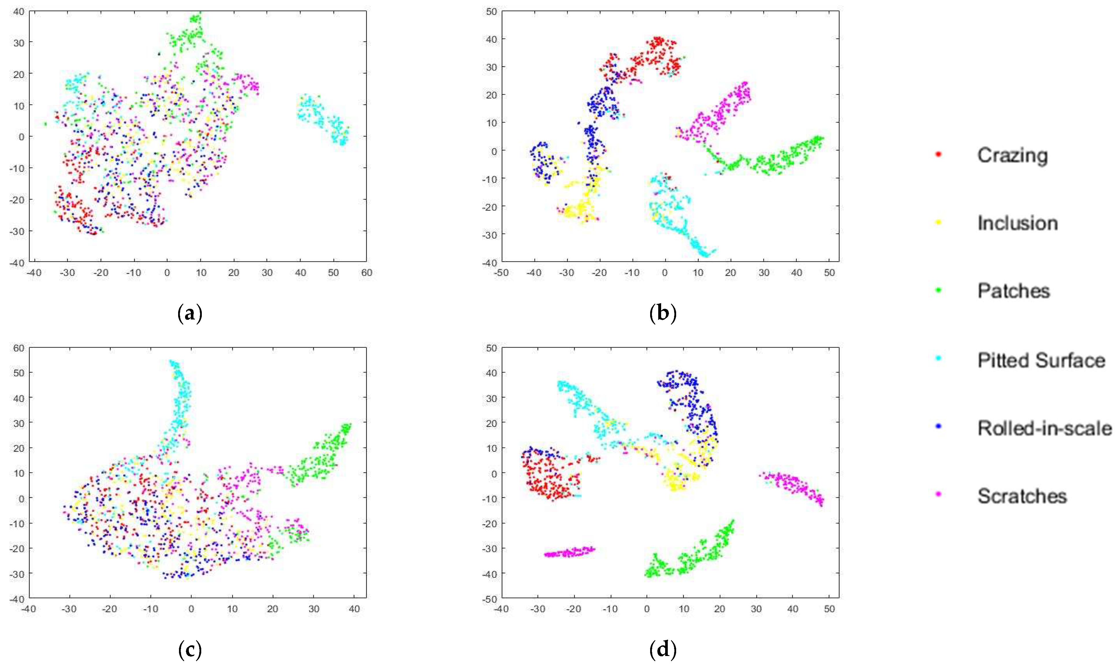
In addition, to visualize the classification performance on the disturbance defect dataset, a nonlinear dimensionality reduction technique, namely t-distributed stochastic neighbor embedding (t-SNE), was adopted to visualize the classification performance on the disturbance defect dataset. Concretely, t-SNE reduced the data dimensionality so that it was easier to interpret and analyze. Besides, the proposed MRFFN adopted multiple inception modules to extract multiscale features and applied the max pooling layer to downsample the aggregate features. Lastly, a fully connected layer was applied to extract all of the discriminative information from the above layers. Hence, the activations of the fully connected layer from both the level 0 and level 1 networks were applied as the feature vectors of the feature visualization to provide a better interpretation of the activations for the decision of interest. Figure 7 and Figure 8 demonstrate the data distribution of the proposed MRFFN on Gaussian white noise and salt and pepper noise datasets. According to the t-SNE maps, it is observed that the original MRFFN could roughly differentiate the majority classes of pitted surface and patches defects. However, the majority classes of crazing, inclusion, rolled-in scale, and scratches were thoroughly mixed with each other. Thus, it can be clearly explained why the original MRFFN yielded the worst performance on the disturbance defect dataset. On the other hand, when the disturbance defect dataset retrained the proposed MRFFN, six clusters could be found clearly in Figure 7, Figure 8 and Figure 9. Therefore, these results indicate that MRFFN shows its robustness when the models are retrained by the disturbance defect dataset.
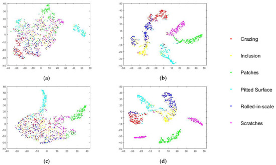
Figure 7.
Feature visualization via t-SNE on Gaussian white noise (Variance 0.3). The feature vectors are extracted from the activations of the fully connected layer. (a) The original level 0 model. (b) The retrained level 0 model. (c) The original level 1 model. (d) The retrained level 1 model.
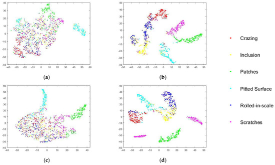
Figure 8.
Feature visualization via t-SNE on salt and pepper noise (Density 0.3). The feature vectors are extracted from the activations of the fully connected layer. (a) The original level 0 model. (b) The retrained level 0 model. (c) The original level 1 model, (d) The retrained level 1 model.
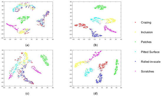
Figure 9.
Feature visualization via t-SNE on motion blur (Motion length 0.3). The feature vectors are extracted from the activations of the fully connected layer. (a) The original level 0 model. (b) The retrained level 0 model. (c) The original level 1 model. (d) The retrained level 1 model.
Furthermore, the experiments were conducted to evaluate the robustness of the MRFFN by comparing it with the other conventional pre-trained DL models, including AlexNet, VGG16, and ResNet-18. According to Table 4, it can be seen that the recognition accuracies of the MRFFN were 98.04% to 85.65%, while the other conventional DL models were 96.45% to 67.24%, 97.73% to 53.35%, and 97.60% to 73.02%, respectively. Obviously, the proposed method outperformed the other DL methods and retained an excellent performance for the variance 0.3 task. For instance, the recognition accuracy gaps of the DL-methods between each variance task were 4.79% to 5.79%, 5.49% to 6.86%, and 13.29% to 33.89% accordingly, while the proposed MRFFN yielded lower accuracy gaps (2.41%, 1.84%, and 8.14%) on the Gaussian white noise tasks. On a similar note, the proposed method had a lower sensitivity to the salt and pepper noise and motion blur compared with the conventional DL methods, which retained an excellent performance of 87.09% and 96.40% accuracies on the density 0.3 and length 20 tasks. To sum up, these results indicate that MRFFN was able to learn more representative features from the limited data, meanwhile suppressing the redundant noise from the raw data.
4.5.2. In-Depth Analysis the Impact of Various Disturbance Factors
To provide an outlook of the influence of each disturbance factor, the proposed method’s confusion matrix on different interference datasets was provided in this experiment. From the confusion matrix, the first row represented the ground truth of the defect category, and the value in each column indicates the prediction result of the proposed method. First, the inclusion achieved the lowest recall (79.60%) and precision (74.62%) among the six kinds of defects based on Table 7. In the variance 0.3 subset, 5.64% inclusion samples were misclassified as rolled-in scale and 13.64% rolled-in scale samples were wrongly classified as inclusion. In addition, 10.20% of inclusion samples were misclassified as pitted surface and 5.92% pitted surface samples were wrongly predicted as inclusion. According to Figure 7b,d, it can be discerned that the minority classes of rolled-in scale, inclusion, and pitted surface were mixed with each other. Thus, the similarity between inclusion, rolled-in scale, and pitted surface was exacerbated while applying Gaussian white noise to the raw data. Furthermore, 5.96% of crazing samples were categorized as rolled-in scale as there were “inter-class” similarity and “intra-class” diversity among the two defects [7]. In Table 8, the overall performance of the proposed method was as similar as the Gaussian white noise dataset. Still, the inclusion achieved the lowest recall (82.00%) and precision (79.74%) results. In addition, the proposed method was influenced by the “inter-class” similarity and “intra-class” between crazing and rolled-in scale defects in the salt and pepper noise subset.
Table 7.
The confusion matrices when adopting the MRFFN+IA method on variance 0.3 task containing six types of defects (%), where Cr, In, Pa, PS, RS, and Sc denote the crazing, inclusion, patches, pitted surface, rolled-in scale, and scratches defects respectively.
Table 8.
The confusion matrices when adopting the MRFFN+IA method on density 0.3 task containing six types of defects (%), where Cr, In, Pa, PS, RS, and Sc denote the crazing, inclusion, patches, pitted surface, rolled-in scale, and scratches defects respectively.
Based on the t-SNE maps in Figure 8b,d, some nodes of inclusion and rolled-in scale, inclusion and pitted surface are very close. Hence, these results lead to misclassifying the MRFFN among the inclusion, pitted surface, and rolled-in scale defects while applying salt and pepper noise. Lastly, the results from Table 9 demonstrate that the models can easily predict the crazing, patches and rolled-in scale defects since these defects achieve high recall. On the contrary, the pitted surface defect achieves the lowest recall among six kinds of defect. (94.12%). According to the examples in Figure 5, it can be observed that the motion blur will stretch the pitted surface defects into long strips which look similar to the inclusion defects. In Figure 9b,d, there are minority classes of pitted surface and scratches, which were misclassified as inclusion class. Hence, the motion blur disturbance factor will deteriorate the misclassification between the pitted surface, scratches, and the inclusion defects.
Table 9.
The confusion matrices when adopting the MRFFN+IA method on motion length 20 task containing six types of defects (%), where Cr, In, Pa, PS, RS, and Sc denote the crazing, inclusion, patches, pitted surface, rolled-in scale, and scratches defects respectively.
5. Discussion
5.1. The Performance of the Higher-Level Gaussian Pyramid
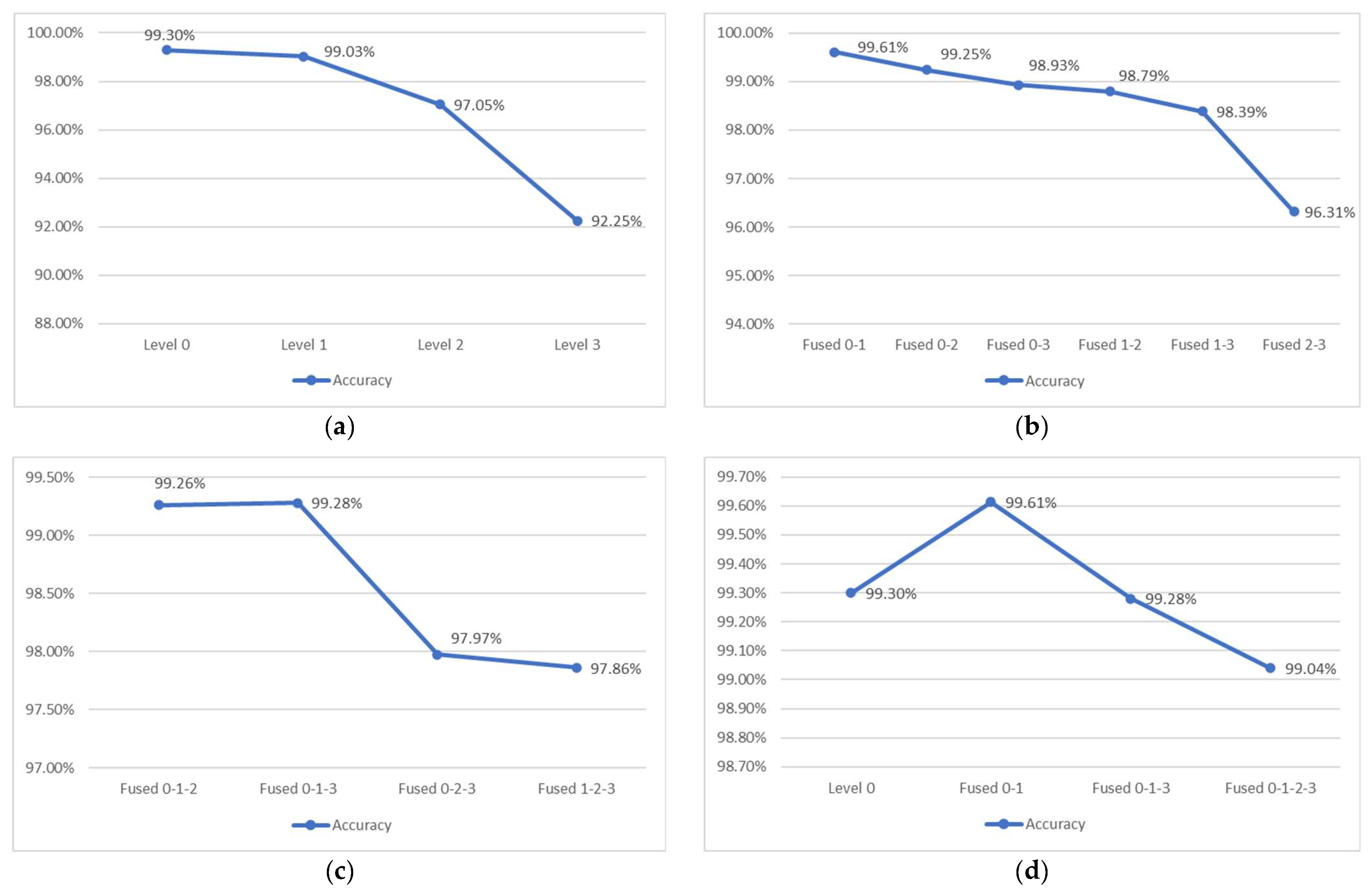
In the proposed method, the Gaussian pyramid can provide a multi-level of sub-images. However, the high-level images are obtained through several low pass filtering and downsampling processes, which implies that the higher level contains more information loss. To investigate whether the model could extract important features from the higher level, this section will discuss the performance of each model and fusion network. Here, the level 1 structure was adopted as the level 2 and level 3 structures, which removed the last two inception modules from the pre-trained GoogLeNet and applied a higher learning rate factor for the shallower layers. According to Figure 10a, the accuracies of the individual networks decreased as higher levels of the Gaussian pyramid were applied, the accuracy gaps between level 1, level 2, and level 3 increased significantly, which indicates that some important features were removed in the high level of the Gaussian pyramid. While comparing the performance between individual networks and fused two networks, the fused 0–1 network achieved the highest accuracy (99.61%) among the fused two networks based on the results in Figure 10b. In contrast, the fused 0–2 and fused 0–3 networks were 0.05% and 0.37% lower than the level 0 network, and the fused 1–2 and fused 1–3 networks were 0.24% and 0.64% lower that the level 1 network. In Figure 10c, the overall performance of the fused three networks was lower than the level 0 network, and the accuracies dropped significantly while applying level 2 and level 3 as the main proportions. These results indicate that the level 2 and level 3 networks were misleading the prediction of the fusion network. Lastly, the greatest performances of the individual network, fused two networks, fused three networks, and fused all networks are compared in Figure 10d. It shows a noticeable peak at the fused 0–1 network, which illustrates that the fused 0–1 yielded the highest accuracy among all of the networks. Besides, the results of the fused three networks, which contained larger training parameters, were not as good as the fused 0–1 network. These results indicate that the fused 0–1 network is able to promote the performance of the individual network, simultaneously surpassing the other large-scale fusion network. As a result, this study utilized level 0 and level 1 of the Gaussian pyramid as the proposed method.
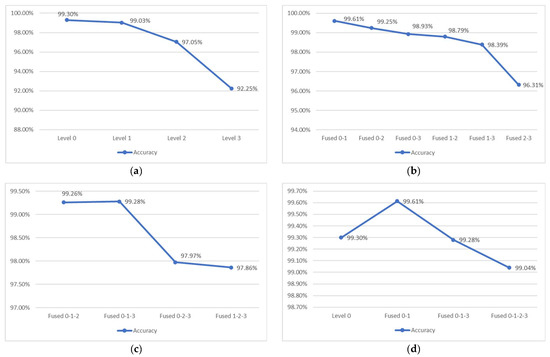
Figure 10.
The accuracies distribution of individual and fused networks based on NEU dataset. (a) Individual network (b). Fused two networks. (c) Fused three networks. (d) Greatest performance of individual and fused networks.
5.2. The Performance of Different Fusion Weights
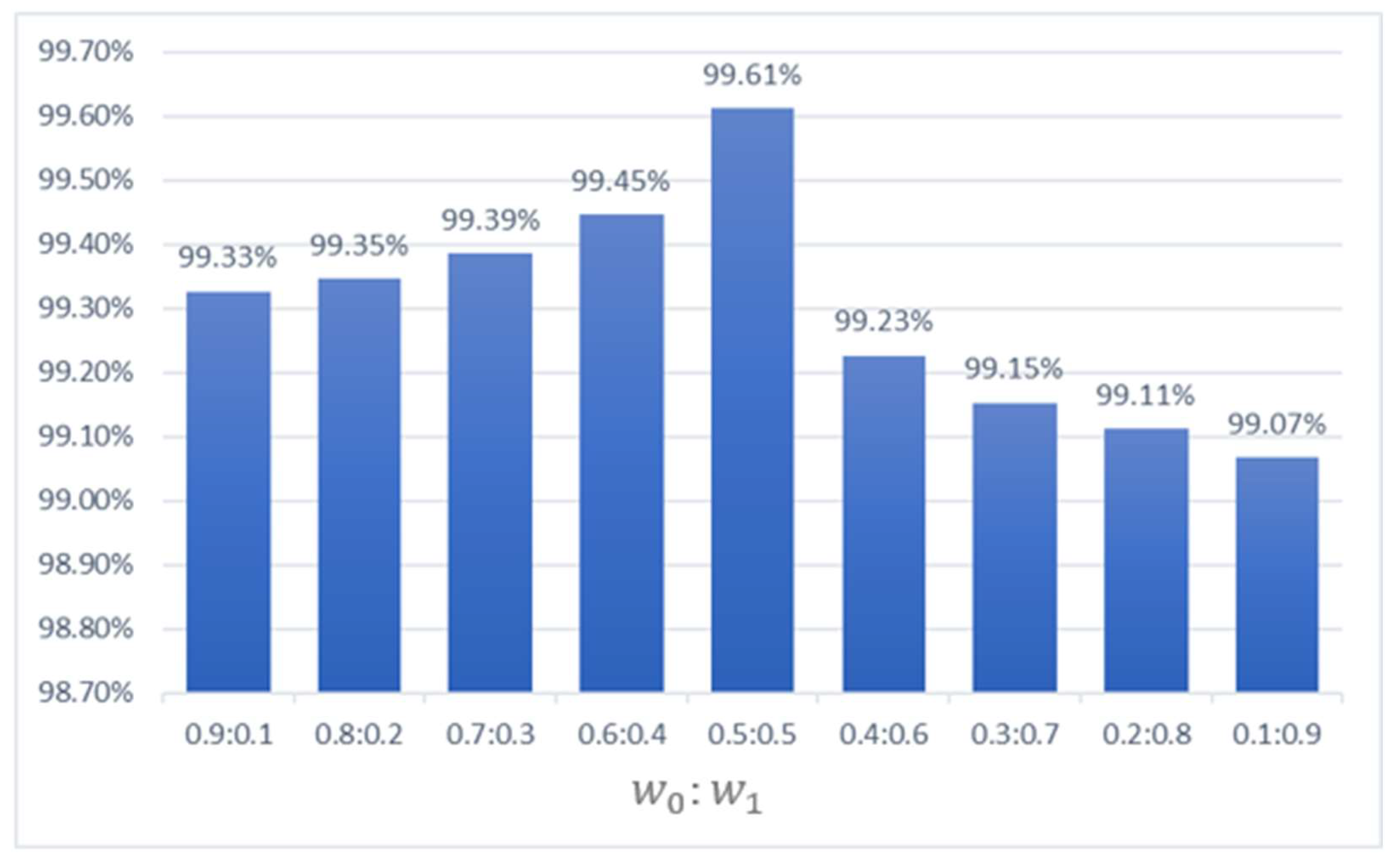
In Section 3.3, the equation of the final prediction result is introduced and both networks had an average weight while calculating the final scores. This section will discuss the performance of fusion networks under different weight circumstances. Here, the weight of the arbitrary network decreased from 0.9 to 0.1 while the other weight increased from 0.1 to 0.9, respectively. In this experiment, all the implementation details were taken according to Section 3.1 and by applying 50 samples from the NEU dataset as the training set. Based on the experiment results, the level 1 models were able to enhance the performance of the level 0 models. According to the report in Section 3.3, the level 0 models had an average accuracy of 99.30%. Hence, the accuracy of the fusion networks was improved when comparing the results below with the level 0 models. Obviously, once the weight of the level 0 models was greater than or equal to the level 1 models, the overall results of the fusion networks was higher than the level 0 models. In Figure 11, it can be seen that the accuracy of the fusion network was increasing when the weight of the level 0 models decreased. The results show that the fusion network had the highest accuracy of 99.61% when applying an average weight for both networks. However, once the level 1 models had a greater influence than the level 0 models, the performance of the fusion networks decreased gradually. Thus, these results indicated that the average weight was the most conducive for improving the performance of both networks. Lastly, in order to solve the divergent results between the fusion networks, the weights of the level 0 and level 1 models were set as 0.6:0.4 when the final results contained the two highest scores, as it achieved the second-highest accuracy among the other weights.
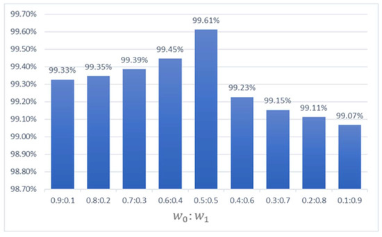
Figure 11.
The performance of different fusion weights. and denote as the fusion weight of level 0 and level 1 models.
6. Conclusions
This paper proposes a novel method to improve the automated defect inspection on a hot rolled steel strip by introducing the multi-receptive field fusion-based network (MRFFN). Here, the Gaussian pyramid is applied to provide more meaningful information from the limited data. Subsequently, two lightweight multi-receptive field networks have been proposed to learn multilevel information. Besides, high learning rate factors are implemented for the shallower layers to accelerate the convergence of the training process and to prevent the gradient vanishing while training the deep networks. The experimental results based on the NEU dataset indicate that the proposed MRFFN only requires small training samples to achieve high accuracy compared with the state-of-the-art. Furthermore, the robustness of the proposed method has been evaluated on the disturbance defect dataset. It can be observed that the proposed method performs significantly better in comparison with the conventional CNN model against Gaussian white noise, salt and pepper noise, and motion blur.
However, there are some limitations in this article. Firstly, the Gaussian pyramid takes several low pass filtering and downsampling processes for the raw images, which implies that the high-level images obtain relatively less information for the training model. Thus, the performance of the training model should be considered to assure that important features are retained in the high-level images. Additionally, the proposed MRFFN requires two deep networks that contain a massive training parameter. Hence, it may impede the efficiency of the inspection speed and require powerful hardware for the high computational load. Therefore, for the future, attention can be devoted to the following direction.First, the PCA can be adopted to eliminate the redundant information from the raw data. Then, a deformable feature extraction technique can be introduced to learn the multiscale features to acquire a more accurate description of image content.
Author Contributions
Conceptualization, K.-C.W.; methodology, K.-C.W., W.-P.T. and S.-T.L.; formal analysis, W.-P.T., S.-T.L.; writing—original draft preparation, W.-P.T. and S.-T.L.; writing—review and editing, C.-C.C., P.-C.H., M.-H.T., Y.-T.T. and S.-H.C. All authors have read and agreed to the published version of the manuscript.
Funding
This research was funded by the Ministry of Science and Technology, Taiwan (MOST 108-2221-E-158-003, MOST 109-2622-E-035-022, MOST 109-2221-E-035-001-MY2, and MOST 109-2221-E-035-065-MY2).
Institutional Review Board Statement
Not applicable.
Informed Consent Statement
Not applicable.
Data Availability Statement
Publicly available datasets were analyzed in this study. The defect dataset can be found here: http://faculty.neu.edu.cn/songkechen/zh_CN/zdylm/263270/list/index.htm, accessed on 9 October 2021.
Acknowledgments
The authors would like to thank for the invaluable feedback from the editors and reviewers.
Conflicts of Interest
The authors declare no conflict of interest.
References
- Song, K.; Yan, Y. A noise robust method based on completed local binary patterns for hot-rolled steel strip surface defects. Appl. Surf. Sci. 2013, 285, 858–864. [Google Scholar] [CrossRef]
- Hao, R.Y. A steel surface defect inspection approach towards smart industrial monitoring. J. Intell. Manuf. 2020, 32, 1833–1843. [Google Scholar] [CrossRef]
- Neogi, N.; Mohata, D.K.; Dutta, P.K. Review of vision-based steel surface inspection systems. EURASIP J. Image Video Process. 2014, 2014, 50. [Google Scholar] [CrossRef] [Green Version]
- Zhang, J.Q.; Kang, X.; Ni, H.J.; Ren, F.J. Surface defect detection of steel strips based on classification priority YOLOv3-dense network. Ironmak. Steelmak. 2020, 48, 547–558. [Google Scholar] [CrossRef]
- Szegedy, C.; Liu, W.; Jia, Y.Q.; Sermanet, P.; Reed, S.; Anguelov, D.; Erhan, D.; Vanhoucke, V.; Rabinovich, A. Going Deeper with Convolutions. In Proceedings of the 2015 IEEE Conference on Computer Vision and Pattern Recognition (CVPR), Boston, MA, USA, 7–12 June 2015; pp. 1–9. [Google Scholar]
- Gao, Y.; Liu, X.; Wang, X.V.; Wang, L.; Gao, L. A Review on Recent Advances in Vision-based Defect Recognition towards Industrial Intelligence. J. Manuf. Syst. 2021. online ahead of print. [Google Scholar] [CrossRef]
- Xie, X.H. A Review of Recent Advances in Surface Defect Detection using Texture analysis Techniques. Electron. Lett. Comput. Vis. Image Anal. 2008, 7, 1–22. [Google Scholar] [CrossRef] [Green Version]
- Gan, Y.S.; Chee, S.S.; Huang, Y.C.; Liong, S.T.; Yau, W.C.; Ruiz, R. Automated leather defect inspection using statistical approach on image intensity. J. Ambient. Intell. Humaniz. Comput. 2020, 12, 1–17. [Google Scholar]
- Kumar, J.; Srivastava, S.P.; Anand, R.S.; Arvind, P.; Bhardwaj, S.; Thakur, A. GLCM and ANN based Approach for Classification of Radiographics Weld Images. In Proceedings of the 2018 IEEE 13th International Conference on Industrial and Information Systems (ICIIS), Rupnagar, India, 1–2 December 2018. [Google Scholar]
- Wang, Y.L.; Xia, H.B.; Yuan, X.F.; Li, L.; Sun, B. Distributed defect recognition on steel surfaces using an improved random forest algorithm with optimal multi-feature-set fusion. Multimed. Tools Appl. 2017, 77, 16741–16770. [Google Scholar] [CrossRef]
- Chondronasios, A.; Popov, I.; Jordanov, I. Feature selection for surface defect classification of extruded aluminum profiles. Int. J. Adv. Manuf. Technol. 2016, 83, 33–41. [Google Scholar] [CrossRef]
- Amid, E.; Aghdam, S.R.; Amindavar, H. Enhanced Performance for Support Vector Machines as Multiclass Classifiers in Steel Surface Defect Detection. Int. J. Electr. Comput. Energetic Electron. Commun. Eng. 2012, 6, 1096–1100. [Google Scholar]
- Liu, Y.; Xu, K.; Xu, J.W. An Improved MB-LBP Defect Recognition Approach for the Surface of Steel Plates. Appl. Sci. 2019, 9, 4222. [Google Scholar] [CrossRef] [Green Version]
- Yan, K.; Dong, Q.; Sun, T.T.; Zhang, M.; Zhang, S.Y. Weld Defect Detection based on Completed Local Ternary Patterns. In ICVIP 2017: Proceedings of the International Conference on Video and Image Processing 2017; ACM: New York, NY, USA, 2017; pp. 6–14. [Google Scholar]
- Chu, M.X.; Gong, R.F.; Gao, S.; Zhao, J. Steel surface defects recognition based on multi-type statistical features and enhanced twin support vector machine. Chemom. Intell. Lab. Syst. 2017, 171, 140–150. [Google Scholar] [CrossRef]
- Lecun, Y.; Bottou, L.; Bengio, Y.; Haffner, P. Gradient-based learning applied to document recognition. In Proceedings of the IEEE 1998, Pasadena, CA, USA, 29 May 1998; Volume 86, pp. 2278–2324. [Google Scholar]
- Masci, J.; Meier, U.; Ciresan, D.; Schmidhuber, J.; Fricout, G. Steel defect classification with Max-Pooling Convolutional Neural Networks. In Proceedings of the 2012 International Joint Conference on Neural Networks (IJCNN), Brisbane, Australia, 10–15 June 2012. [Google Scholar]
- Khumaidi, A.; Yuniarno, E.M.; Purnomo, M.H. Welding defect classification based on convolution neural network (CNN) and Gaussian kernel. In Proceedings of the 2017 International Seminar on Intelligent Technology and Its Applications (ISITIA), Surabaya, Indonesia, 28–29 August 2017. [Google Scholar]
- Lee, S.Y.; Tama, B.A.; Moon, S.J.; Lee, S.C. Steel Surface Defect Diagnostics Using Deep Convolutional Neural Network and Class Activation Map. Appl. Sci. 2019, 9, 5449. [Google Scholar] [CrossRef] [Green Version]
- Yang, Y.T.; Pan, L.H.; Ma, J.X.; Yang, R.Z.; Zhu, Y.S.; Yang, Y.Z.; Zhang, L. A High-Performance Deep Learning Algorithm for the Automated Optical Inspection of Laser Welding. Appl. Sci. 2020, 10, 933. [Google Scholar] [CrossRef] [Green Version]
- He, D.; Xu, K.; Zhou, P. Defect detection of hot rolled steels with a new object detection framework called classification priority network. Comput. Ind. Eng. 2019, 128, 290–297. [Google Scholar] [CrossRef]
- Fu, G.Z.; Sun, P.Z.; Zhu, W.B.; Yang, J.X.; Cao, Y.L.; Yang, M.Y.; Cao, Y.P. A deep-learning-based approach for fast and robust steel surface defects classification. Opt. Lasers Eng. 2019, 121, 397–405. [Google Scholar] [CrossRef]
- Chen, W.; Gao, Y.P.; Gao, L.; Li, X.Y. A New Ensemble Approach based on Deep Convolutional Neural Networks for Steel Surface Defect classification. Procedia CIRP 2018, 72, 1069–1072. [Google Scholar] [CrossRef]
- Ren, R.X.; Hung, T.; Tan, K.C. A Generic Deep-Learning-Based Approach for Automated Surface Inspection. IEEE Trans. Cybern. 2018, 48, 929–940. [Google Scholar] [CrossRef]
- Wang, T.; Chen, Y.; Qiao, M.; Snoussi, H. A fast and robust convolutional neural network-based defect detection model in product quality control. Int. J. Adv. Manuf. Technol. 2018, 94, 3465–3471. [Google Scholar] [CrossRef]
- Wang, Y.B.; Huang, J.K.; Wang, Y.; Feng, S.H.; Peng, T.; Yang, H.Y.; Zou, J. A CNN-Based Adaptive Surface Monitoring System for Fused Deposition Modeling. IEEE/ASME Trans. Mechatron. 2020, 25, 2287–2296. [Google Scholar] [CrossRef]
- He, H.; Xu, K.; Wang, D.D. Design of multi-scale receptive field convolutional neural network for surface inspection of hot rolled steels. Image Vis. Comput. 2019, 89, 12–20. [Google Scholar] [CrossRef]
- He, Y.; Song, K.C.; Dong, H.W.; Yan, Y.H. Semi-supervised defect classification of steel surface based on multi-training and generative adversarial network. Opt. Lasers Eng. 2019, 122, 294–302. [Google Scholar] [CrossRef]
- Gao, Y.P.; Gao, L.; Li, X.Y.; Yan, X.G. A semi-supervised convolutional neural network-based method for steel surface defect recognition. Robot. Comput. Integr. Manuf. 2020, 61, 101825. [Google Scholar] [CrossRef]
- Yun, J.P.; Shin, W.C.; Koo, G.W.; Kim, M.S.; Lee, C.K.; Lee, S.J. Automated defect inspection system for metal surfaces based on deep learning and data augmentation. J. Manuf. Syst. 2020, 55, 317–324. [Google Scholar] [CrossRef]
- Le, X.Y.; Mei, J.H.; Zhang, H.D.; Zhou, B.Y.; Xi, J.T. A learning-based approach for surface defect detection using small image datasets. Neurocomputing 2020, 408, 112–120. [Google Scholar] [CrossRef]
- Gao, Y.P.; Gao, L.; Li, X.Y. A Generative Adversarial Network Based Deep Learning Method for Low-Quality Defect Image Reconstruction and Recognition. IEEE Trans. Ind. Inform. 2021, 17, 3231–3240. [Google Scholar] [CrossRef]
- Zhang, C.; Shi, W.; Li, X.F.; Zhang, H.J.; Liu, H. An Improved Bare PCB Defect Detection Approach Based on Deep Feature Learning. J. Eng. 2018, 2018, 1415–1420. [Google Scholar] [CrossRef]
- Tabernik, D.; Šela, J.; Skvarč, J.; Skočaj, D. Segmentation-Based Deep-Learning Approach for Surface-Defect Detection. J. Intell. Manuf. 2020, 31, 759–776. [Google Scholar] [CrossRef] [Green Version]
- Feng, S.; Zhou, H.Y.; Dong, H.B. Using deep neural network with small dataset to predict material defects. Mater. Des. 2019, 162, 300–310. [Google Scholar] [CrossRef]
- Ajmi, C.; Zapata, J.; Martínez-Álvarez, J.J.; Doménech, G.; Ruiz, R. Using Deep Learning for Defect Classification on a Small Weld X-ray Image Dataset. J. Nondestruct. Eval. 2020, 39, 68. [Google Scholar] [CrossRef]
- Gao, Y.P.; Gao, L.; Li, X.Y.; Wang, X.V. A Multilevel Information Fusion-Based Deep Learning Method for Vision-Based Defect Recognition. IEEE Trans. Instrum. Meas. 2020, 69, 3980–3991. [Google Scholar] [CrossRef]
- Wan, X.; Zhang, X.Y.; Liu, L.L. An Improved VGG19 Transfer Learning Strip Steel Surface Defect Recognition Deep Neural Network Based on Few Samples and Imbalanced Datasets. Appl. Sci. 2021, 11, 2606. [Google Scholar] [CrossRef]
- Adelson, E.H.; Anderson, C.H.; Bergn, J.R.; Burt, P.J.; Ordern, J.M. Pyramid methods in image processing. RCA Eng. 1984, 29, 33–41. [Google Scholar]
- Chen, H.Y.; Pang, Y.; Hu, Q.D.; Liu, K. Solar Cell Surface Defect Inspection Based on Multispectral Convolutional Neural Network. J. Intell. Manuf. 2020, 31, 453–468. [Google Scholar] [CrossRef] [Green Version]
- Zhong, Z.Y.; Jin, L.W.; Xie, Z.C. High Performance Offline Handwritten Chinese Character Recognition Using GoogLeNet and Directional Feature Maps. In Proceedings of the 2015 13th International Conference on Document Analysis and Recognition (ICDAR), Tunis, Tunisia, 23–26 August 2015; pp. 846–850. [Google Scholar]
- Singla, A.; Yuan, L.; Ebrahimi, T. Food/Non-food Image Classification and Food Categorization using Pre-Trained GoogLeNet Model. In Proceedings of the MADiMa’16: Proceedings of the 2nd International Workshop on Multimedia Assisted Dietary Management 2016, Amsterdam, The Netherlands, 16 October 2016; pp. 3–11. [Google Scholar]
- Krizhevsky, A.; Sutskever, I.; Hinton, G.E. ImageNet Classification with Deep Convolutional Neural Networks. Adv. Neural Inf. Process. Syst. 2012, 25, 1097–1105. [Google Scholar] [CrossRef]
- Simonyan, K.; Zisserman, A. Very Deep Convolutional Networks for Large-Scale Image Recognition. In Proceedings of the International Conference on Learning Representations (ICLR), San Diego, CA, USA, 7–9 May 2015. [Google Scholar]
- Kingma, D.P.; Ba, J. A method for stochastic optimization. In Proceedings of the 3rd International Conference on Learning Representations (ICLR), San Diego, CA, USA, 7–9 May 2015. [Google Scholar]
- Luo, Q.W.; Fang, X.X.; Su, J.J.; Zhou, J.; Zhou, B.X.; Yang, C.; Liu, L.; Gui, W.; Tian, L. Automated Visual Defect Classification for Flat Steel Surface: A Survey. IEEE Trans. Instrum. Meas. 2020, 69, 9329–9349. [Google Scholar] [CrossRef]
- Xiao, M.; Jiang, M.M.; Li, G.Y.; Xie, L.; Yi, L. An evolutionary classifier for steel surface defects with small sample set. EURASIP J. Image Video Process. 2017, 2017, 48. [Google Scholar] [CrossRef] [Green Version]


Publisher’s Note: MDPI stays neutral with regard to jurisdictional claims in published maps and institutional affiliations. |
© 2021 by the authors. Licensee MDPI, Basel, Switzerland. This article is an open access article distributed under the terms and conditions of the Creative Commons Attribution (CC BY) license (https://creativecommons.org/licenses/by/4.0/).