Hardware-in-the-Loop Test of a Prosthetic Foot

Abstract

For a targeted development process of foot prostheses, a profound understanding of the dynamic interaction between humans and prostheses is necessary. In engineering, an often employed method to investigate the dynamics of mechanical systems is Hardware-in-the-Loop (HiL). This study conducted a fundamental investigation of whether HiL could be an applicable method to study the dynamics of an amputee wearing a prosthesis. For this purpose, a suitable HiL setup is presented and the first-ever HiL test of a prosthetic foot performed. In this setup, the prosthetic foot was tested on the test bench and coupled in real-time to a cosimulation of the amputee. The amputee was modeled based on the Virtual Pivot Point (VPP) model, and one stride was performed. The Center of Mass (CoM) trajectory, the Ground Reaction Forces (GRFs), and the hip torque were qualitatively analyzed. The results revealed that the basic gait characteristics of the VPP model can be replicated in the HiL test. Still, there were several limitations in the presented HiL setup, such as the limited actuator performance. The results implied that HiL may be a suitable method for testing foot prostheses. Future work will therefore investigate whether changes in the gait pattern can be observed by using different foot prostheses in the HiL test.

1. Introduction

An important purpose of prostheses is to emulate the function of a lost limb and facilitate the independent life of the user [1]. In this paper, the focus is placed on foot prostheses. The purpose of the foot in walking and standing is diverse. Active balancing, body weight support, adapting to different terrain, and pushing off the ground for propulsion are some of the foot’s functions [2]. Mimicking the foot’s function with a prosthetic foot is challenging, which causes an altered gait pattern of amputees compared to able-bodied humans [3]. The remaining intact body parts are used to compensate for the lost functionality, which leads to excessive loading. Typical consequences for prosthesis wearers are a shorter stance time on the amputated leg, slower gait velocities, and increased energy consumption. Furthermore, changes in foot placement and a lift of the hip during swing phase are observed. As a result, this compensatory behavior can lead to serious long-term consequences, such as osteoarthritis, osteoporosis, and back pain [4]. To improve prosthetic feet further and minimize these side effects, the understanding of how amputees adapt to different prosthetic feet needs to be enhanced. Testing procedures that include the dynamic interaction between the amputee and a prosthesis are therefore desired.

In the industry, a variety of test methods are commonly used. For the approval of prostheses, standardized test procedures are defined in ISO 10328, ISO 22523, ISO 22675, and ISO 16955 [5,6]. These procedures include strength tests and tests of the dynamic loading conditions during heel to toe movement. However, these tests do not consider the interaction between the prosthesis and the user, i.e., how certain properties benefit a user. Further testing methods commonly applied can be classified into model-based, human-based, and robot-based testing [7]. While model-based testing can be performed in the early development stage, the modeling process is complex and the validation of the models is difficult [1,8]. Human-based testing offers a great insight into the gait dynamics of amputees and the dynamic interplay between a user and the prosthesis [7,9]. However, the drawbacks of human-based testing are that the results are subjective and not repeatable [10,11]. In addition, the safety of the subjects is always paramount, leading to a limitation of possible testing scenarios. Robot-based testing is an objective and repeatable approach to test prosthetic feet [10]. These tests do not take the dynamic interplay between the prosthesis and the amputee into account, however. This means that the loading trajectory of the robot does not adapt depending on the resulting forces of the prosthesis, which a human would do (posture, walking speed, etc.).

All of these test methods have their advantages and shortcomings. Ideally, a testing procedure is robot-based—due to the objectivity, the possibility to measure different quantities easily, the test repeatability and because no test subjects are required—while still emulating the dynamics of the prosthesis wearer. A novel approach for testing of foot prostheses could therefore be Hardware-in-the-Loop (HiL). HiL is a combination of model-based and robot-based testing, where the amputee is modeled and the prosthetic foot is tested experimentally. Human modeling is extremely complex and requires a great understanding of gait dynamics. The modeling of the human gait requires some simplifications. Nevertheless, a HiL approach allows studying the dynamic interaction without the need for test subjects. The modeled amputee and the prosthetic foot exchange information in real-time to couple them, that is to analyze their dynamic interplay. This idea is visualized in Figure 1.

While the idea of testing prosthetic feet using HiL was already proposed before by [7,11], the realization/implementation has not been performed yet. This paper therefore literally aims at taking this first step, i.e., implementing a HiL test for prosthetic feet. Specifically, the aim of this article is to show the basic feasibility of conducting a HiL test that is able to replicate the dynamic interaction between an amputee and a prosthesis. This first proof-of-concept makes use of a simple human gait model that is able to emulate the gait characteristics during the stance phase. A modified version of the Virtual Pivot Point (VPP) model is used in this work to simulate the amputee, and one gait cycle is performed. We hypothesized that the results of the HiL test would qualitatively resemble the gait characteristics of the VPP model and therefore emulate human gait dynamics.

The remainder of the paper is structured as follows. The groundwork with an introduction to HiL and human gait modeling is laid in Section 2. In Section 3, the implementation is described. For that purpose, the model of the amputee is explained and the Equations of Motion (EoMs) are derived. Furthermore, the parameters used and the experimental setup are described. The results of one gait cycle are presented and discussed critically in Section 4. Finally, a brief summary of the paper is given and a conclusion is drawn in Section 5.

2. State-of-the-Art

This section introduces HiL and sets the notation for this article. For the realization of the HiL setup, the amputee needs to be modeled. This work makes use of a gait model found in the literature of biomechanics.

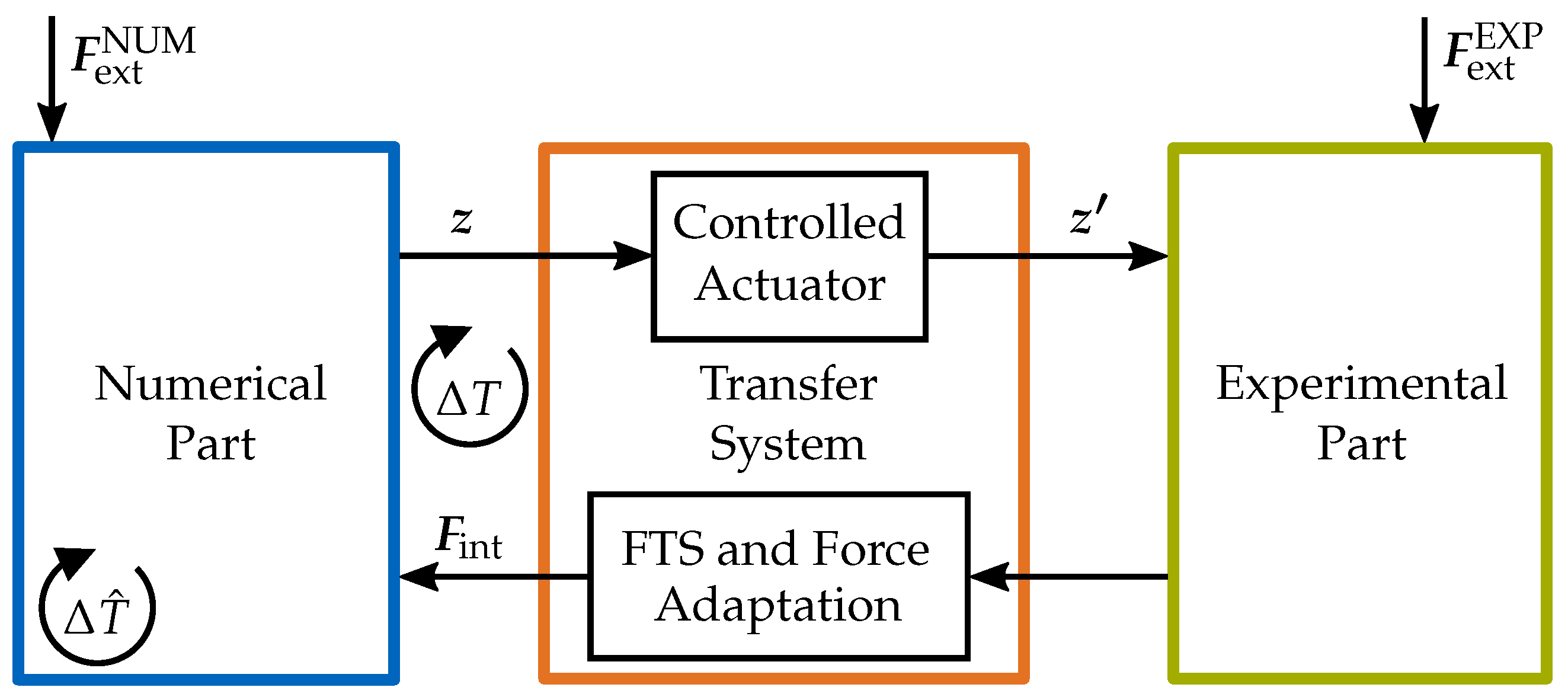
2.1. Fundamentals of Hardware-in-the-Loop

In Hardware-in-the-Loop (HiL), critical components are tested experimentally (experimental part) and coupled in real time with a simulation of the surrounding mechanical system (numerical part). Due to the coupling, the critical components are tested with realistic boundary impedance, and the loading of the components in the test is the same as it will be in real operation. In this work, mechanical-level HiL (denoted as HiL) was employed, which is also called real-time hybrid substructuring/simulation in the literature [13]. In mechanical-level HiL, the dynamical interaction between components of a system is analyzed by the exchange of force and displacement/velocity information. The coupling is performed by the transfer system, which comprises a controlled actuator, a Force–Torque Sensor (FTS), and a Digital Signal Processor (DSP).

The standard signal flow to couple the numerical and experimental parts is as follows; cf. Figure 2. The explanations are given for the special case of one numerical and one experimental part, as this is the case in this work.

The numerical model solves for the interface Degrees of Freedom (DoFs) (Vectors are indicated by variables written in bold. Variables printed in normal type are scalars.) $\mathbf{z}$ using a numerical time integration scheme, typically with a fixed sampling time of $\Delta \widehat{T}$. The actuator performs the position command and excites the experimentally tested component by the achieved motion ${\mathbf{z}}^{\prime }$. Due to this loading, interface forces ${\mathit{F}}_{\mathbf{int}}$ build and can be measured by the FTS. The block Force Adaptation denotes any filtering of the measured signals or transformations of the coordinate system. The measured interface forces are used for the next time integration step. The numerical, as well as the experimental part can be excited by external forces, which are denoted by ${\mathit{F}}_{\mathrm{ext}}^{\mathrm{NUM}}$ and ${\mathit{F}}_{\mathrm{ext}}^{\mathrm{EXP}}$, respectively. The exchange of displacement and force information is performed at a fixed sampling time, which is the synchronization time step $\Delta T$.

HiL testing of foot prostheses has not been reported so far, and the purpose of this work was to set the foundation for such tests. This application of HiL is particularly challenging because of the transition from noncontact to contact, requiring a very robust control of the transfer system.

2.2. Basic Human Gait Models

Based on data from gait laboratories, various walking and running models have been proposed to describe the gait pattern. The HiL test requires a model of the amputee that implements basic gait characteristics. Furthermore, the model needs to be solved in real time, i.e., within the sample time $\Delta \widehat{T}$. For this first proof-of-concept study, a model with low complexity while still being able to represent basic gait characteristics was sought.

Walking is a repetitive motion, and the movement and time interval between two successive events is called the Gait Cycle (GC). In this work, the GC starts when the Center of Mass (CoM) is above the left foot and terminates one stride later, i.e., at the next midstance of the left foot. During this GC, the left, as well as the right foot pass through the stance phase ($60\%$ of the GC) and the swing phase ($40\%$ of the GC). The CoM motion resembles a sinusoidal motion with a magnitude of $0.032\pm 0.008 \mathrm{m}$ during a GC [14]. A further fundamental gait characteristic is the shape of the Ground Reaction Forces (GRFs) in the horizontal (x) and vertical (y) direction. The GRFs are the forces that the ground exerts on the body. In the horizontal direction, a point symmetric force profile is observed, where decelerating forces (negative x direction) are measured in the first part of the stance phase and accelerating forces are measured in the second half of the stance phase (positive x direction). Typically, the shape of the GRFs in the vertical direction exhibits a double-hump shape, with a minimum between the two humps (m-shape) [14,15,16,17].

This work made use of the two-dimensional Virtual Pivot Point (VPP) model by Maus et al. [18], which is based on the Spring-Loaded Inverted Pendulum (SLIP) template model [19].

The model is illustrated in Figure 3. The upper body is represented as a trunk, where the whole body mass is concentrated. The legs are modeled by massless springs. This model was based on the observations that the GRFs intersecting in one or more points above the CoM, resulting in a constellation similar to a physical pendulum [20]. This intersection point is observed in humans on treadmills (Note that the VP is only observed during the single support phase in humans [21]. However, the VPP model assumes that the GRFs are also redirected into the VPP during the double-support phase.) and animals such as dogs and chickens. The principle is named the Virtual Pendulum (VP), as it stabilizes the trunk orientation. The VP principle was implemented in the VPP model. In this model, the GRFs are actively redirected into the VPP by the implementation of an additional hip torque ${\tau }_{\mathrm{V}\mathrm{P}\mathrm{P},\mathrm{j}}$ (with $\mathrm{j}=\{\mathrm{L},\mathrm{R}\}$ for the left and right leg) [18,22].

The resulting hip torque is calculated for each leg $\mathrm{j}=\{\mathrm{L},\mathrm{R}\}$ independently during contact with the ground by:

$$\begin{array}{c}\hfill {\tau }_{\mathrm{V}\mathrm{P}\mathrm{P},\mathrm{j}}=F_{\tau ,\mathrm{j}}{l}_{\mathrm{j}}\mathrm{with}{F}_{\tau ,\mathrm{j}}=F_{\mathrm{s},\mathrm{j}}tan\left({\gamma }_{\mathrm{V}\mathrm{P}\mathrm{P},\mathrm{j}}\right)=k_{\mathrm{j}}(l_0,\mathrm{j}-l_{\mathrm{j}})tan\left({\gamma }_{\mathrm{V}\mathrm{P}\mathrm{P},\mathrm{j}}\right).\end{array}$$

(1)

Here, $l_0,\mathrm{j}$ and $l_{\mathrm{j}}$ describe the initial and current leg length, and the leg stiffness is denoted by $k_{\mathrm{j}}$. The required $F_{\tau ,\mathrm{j}}$ to redirect the leg forces $F_{\mathrm{s}},\mathrm{j}$ into the VPP depend on the angle ${\gamma }_{\mathrm{V}\mathrm{P}\mathrm{P},\mathrm{j}}$ between the leg axis and the connection of the foot point $x_{\mathrm{F}\mathrm{P},\mathrm{j}}$ to the VPP location (the equations describing the calculation of $l_{\mathrm{j}}$, ${\gamma }_{\mathrm{V}\mathrm{P}\mathrm{P},\mathrm{j}}$, etc., are given in Appendix A). The total GRFs result:

$$\begin{array}{cc}\hfill GR{F}_{\mathrm{j}}& =\sqrt{F_{\mathrm{s},\mathrm{j}}^2+F_{\tau ,\mathrm{j}}^2}=F_{\mathrm{s},\mathrm{j}}\sqrt{1+{tan}^2\left({\gamma }_{\mathrm{V}\mathrm{P}\mathrm{P},\mathrm{j}}\right)}\hfill \end{array}$$

(2)

$$\begin{array}{cc}\hfill GR{F}_{\mathrm{j},x}& =GR{F}_{\mathrm{j}}{\displaystyle \frac{x_{\mathrm{h}}-x_{\mathrm{F}\mathrm{P},\mathrm{j}}}{l_{\mathrm{j}}}}\hfill \end{array}$$

(3)

$$\begin{array}{cc}\hfill GR{F}_{\mathrm{j},y}& =GR{F}_{\mathrm{j}}{\displaystyle \frac{y_{\mathrm{h}}}{l_{\mathrm{j}}}},\hfill \end{array}$$

(4)

where the indices ${(·)}_x$ and ${(·)}_y$ denote the projections of the forces into the x and y direction and the index ${(·)}_{\mathrm{h}}$ denotes the hip joint. The GRFs are calculated when the leg is on the ground, i.e., between Touch Down (TD) and Take Off (TO). As the legs are massless, they do not contribute to the dynamics during the swing phase and their GRFs are zero. After TO, the VPP model assumes that the leg is instantaneously repositioned with a TD angle ${\alpha }_0$. This TD angle is defined by the user.

Using Equations (3) and (4), as well as the gravitational forces on the CoM $m_{\mathrm{V}\mathrm{P}\mathrm{P}}$ and the moment of inertia $J_{\mathrm{V}\mathrm{P}\mathrm{P}}$, the EoMs result:

$$\begin{array}{cc}\hfill m_{\mathrm{V}\mathrm{P}\mathrm{P}}\ddot{x}& ={GRF}_{\mathrm{L},x}+{GRF}_{\mathrm{R},x}\hfill \end{array}$$

(5)

$$\begin{array}{cc}\hfill m_{\mathrm{V}\mathrm{P}\mathrm{P}}\ddot{y}& ={GRF}_{\mathrm{L},y}+{GRF}_{\mathrm{R},y}-m_{\mathrm{V}\mathrm{P}\mathrm{P}}g\hfill \end{array}$$

(6)

$$\begin{array}{cc}\hfill -J_{\mathrm{V}\mathrm{P}\mathrm{P}}{\ddot{\varphi }}_{\mathrm{V}\mathrm{P}\mathrm{P}}& =r_{\mathrm{V}\mathrm{P}\mathrm{P}}\left(sin\left({\varphi }_{\mathrm{V}\mathrm{P}\mathrm{P}}\right)({GRF}_{\mathrm{L},y}+{GRF}_{\mathrm{R},y})-cos\left({\varphi }_{\mathrm{V}\mathrm{P}\mathrm{P}}\right)({GRF}_{\mathrm{L},x}+{GRF}_{\mathrm{R},x})\right).\hfill \end{array}$$

(7)

The principle of angular momentum can also be set up differently, as is described in Appendix B. The VPP model is able to replicate the CoM motion, the shape of the GRFs, as well as the shape of the hip torque observed in humans [18]. Due to the VPP controller (hip torques ${\tau }_{\mathrm{V}\mathrm{P}\mathrm{P},\mathrm{j}}$), the model is able to stabilize the trunk and overcome some disturbances, such as small steps. Still, this is a simple conceptual model representing human gait dynamics.

3. Experimental Setup and Parameters

This section presents the full HiL setup used to perform one stride. The numerical part, which consisted of the modeled amputee, the transfer system used, and the experimental part, are described. Additionally, all parameters are given.

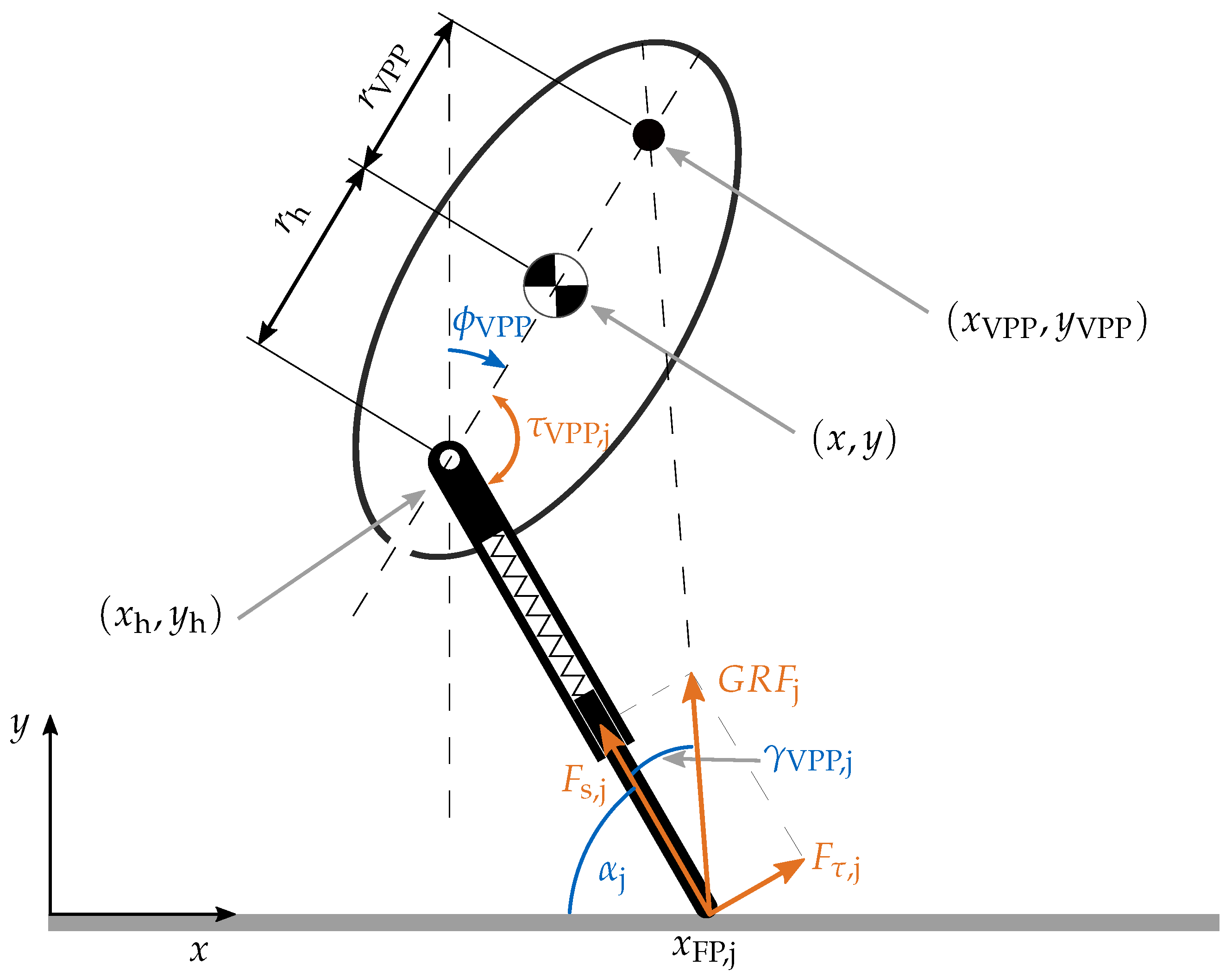
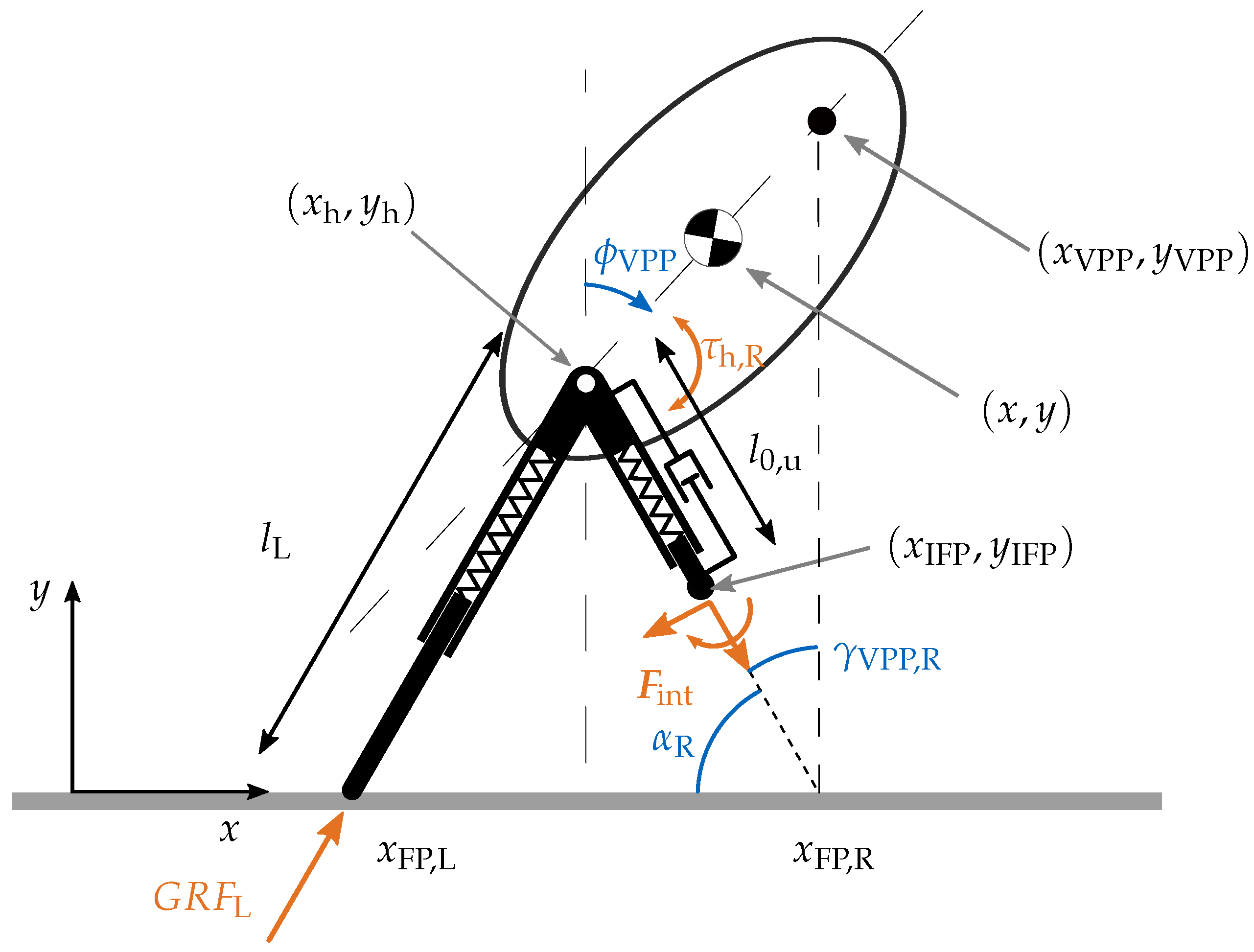
3.1. Modeling an Amputee Using the VPP Model

The VPP model, which is described in Section 2.2, models the gait dynamics of an able-bodied person. Because the HiL setup requires a model of an amputee, this model needs to be modified. These modifications are described in the following.

3.1.1. Model of the Amputated Leg

To model the amputee, the right leg (index R) is cut at the ankle, which is the interface location in this HiL setup. The total leg length of the right leg is $l_{\mathrm{R}}$, which results from the height of the prosthetic foot ${\mathrm{h}}_{\mathrm{f}}$ and the leg length of the remaining leg $l_{\mathrm{u}}$ (resting spring length $l_{0,\mathrm{u}}$; index ${(·)}_{\mathrm{u}}$ denotes the upper part of the amputated leg). In the HiL setup, the prosthetic foot needs to be moved according to the end point of the amputated leg. However, it is numerically not trivial to calculate this position. This is because the amputated leg and the prosthetic foot are as two springs in series, which have to experience the same force. Since the stiffness of the prosthetic foot is not known, the interface location between the amputated leg and the prosthetic foot cannot be calculated. Therefore, an additional DoF is inserted by adding a point mass $m_{\mathrm{I}\mathrm{F}\mathrm{P}}$ at the ankle [24]. Taking a very small value for that mass compared to the model mass ($m_{\mathrm{I}\mathrm{F}\mathrm{P}}\ll m_{\mathrm{V}\mathrm{P}\mathrm{P}}$), the system dynamics are barely modified. This point is called the Interface Point (IFP) at the location $(x_{\mathrm{I}\mathrm{F}\mathrm{P}},y_{\mathrm{I}\mathrm{F}\mathrm{P}})$. The mass IFP forms a vibratory system and introduces artificial high-frequency dynamics. To dampen these oscillations of this point mass, an additional damper with damping constant $d_{\mathrm{u}}$ is inserted in the remaining leg. The modified VPP model is shown in Figure 4.

As described in Section 2.1, measured interface forces ${\mathit{F}}_{\mathbf{int}}$ are the input to the simulation model (in this model, the external forces ${\mathit{F}}_{\mathrm{ext}}^{\mathrm{NUM}}$ only include the gravitational forces). As this model is a two-dimensional model, the vector ${\mathit{F}}_{\mathbf{int}}$ comprises two forces and one torque. In this application, this is a force parallel to the leg axis $F_{\mathrm{int},\Vert }$, a force orthogonal to the leg axis $F_{\mathrm{int},\perp }$, and a torque about the z axis $M_{\mathrm{int}}$.

The motion of the interface mass point is restricted to the leg axis, and the gravitational forces acting on it are neglected. The internal dynamics of the leg with the added IFP and damper are written as:

$$m_{\mathrm{I}\mathrm{F}\mathrm{P}}{\ddot{l}}_{\mathrm{u}}=F_{\mathrm{int},\Vert }-d_{\mathrm{u}}{\dot{l}}_{\mathrm{u}}-k_{\mathrm{u}}(l_{\mathrm{u}}-l_{0,\mathrm{u}})=F_{\mathrm{int},\Vert }-F_{\mathrm{u}}.$$

(8)

In this equation, the forces of the spring-damper element are abbreviated as $F_{\mathrm{u}}$. Note that the dissipated energy of the damper is assumed to be negligible compared to the total system energy of the modeled amputee and therefore not compensated.

3.1.2. Center of Pressure Shift

The idea of the VPP model is that the GRFs always point to the VPP. To calculate the required hip torque, the location where the GRFs are applied needs to be known. In the simple VPP model of Section 2.2, the point of application of the GRFs was easy to find since the leg was supposed to make contact with the ground at a single point $x_{\mathrm{F}\mathrm{P},\mathrm{j}}$ corresponding to the intersection between the ground and the leg axis. When a foot is considered, the point of application of the forces is not necessarily anymore on the axis of the leg since the point of contact between the foot and the ground can travel during the stance phase. In human walking, a shift of this point from the heel to the toes during the stance phase can be observed, and this point is called the Center of Pressure (CoP) [25]. The CoP of the right foot is henceforth denoted by $x_{\mathrm{C}\mathrm{o}\mathrm{P},\mathrm{R}}$, and the foot point $x_{\mathrm{F}\mathrm{P},\mathrm{R}}$ marks the intersection of the leg axis with the ground. The location of the CoP is necessary for the calculations of the modeled amputee due to the required angle ${\gamma }_{\mathrm{V}\mathrm{P}\mathrm{P},\mathrm{R}}$. This angle is defined as the angle between the leg axis (here: connection $x_{\mathrm{C}\mathrm{o}\mathrm{P},\mathrm{R}}$ and $(x_{\mathrm{h}},y_{\mathrm{h}})$) and the connection between the CoP and the VPP (here: connection $x_{\mathrm{C}\mathrm{o}\mathrm{P},\mathrm{R}}$ and $(x_{\mathrm{V}\mathrm{P}\mathrm{P}},y_{\mathrm{V}\mathrm{P}\mathrm{P}})$). The geometry and the forces acting on the foot are illustrated in Figure 5.

How the CoP shifts from the heel to the toes needs to be prescribed (The CoP location could also be determined from a torque equilibrium about the ankle joint using the measured forces and torques. This approach offers some difficulties: firstly, the inertial forces need to be determined, and secondly, our experiments revealed that the noise in the force measurement leads to a noisy calculation of the CoP location). This work assumed a CoP shift depending on the angle ${\alpha }_{\mathrm{R}}$ between the leg and the ground. The implemented relationship is written as:

$$\begin{array}{cc}\hfill x_{\mathrm{C}\mathrm{o}\mathrm{P},\mathrm{R}}& =\left\{\begin{array}{cc}\frac{l_{\mathrm{h}}}{\frac{\pi }{2}-{\alpha }_0}{\alpha }_{\mathrm{R}}+c_1,\hfill & \mathrm{for}{\alpha }_{\mathrm{R}}\le \frac{\pi }{2}\hfill \\ \frac{l_{\mathrm{ff}}}{{\alpha }_{\mathrm{T}\mathrm{O}}-\frac{\pi }{2}}{\alpha }_{\mathrm{R}}+c_2,\hfill & \mathrm{for}{\alpha }_{\mathrm{R}}>\frac{\pi }{2},\hfill \end{array}\right.\hfill \end{array}$$

(9)

using the TD angle ${\alpha }_0$, as well as the geometric dimensions of the foot $l_{\mathrm{h}}$ and $l_{\mathrm{ff}}$ (see Figure 5b). Furthermore, an assumption of the TO angle ${\alpha }_{\mathrm{T}\mathrm{O}}$ is required. The constants $c_1$ and $c_2$ are found using $x_{\mathrm{C}\mathrm{o}\mathrm{P},\mathrm{R}}=x_{\mathrm{F}\mathrm{P},\mathrm{R}}$ at ${\alpha }_{\mathrm{R}}=\frac{\pi }{2}$. This CoP shift is also implemented for the left, intact leg ($x_{\mathrm{F}\mathrm{P},\mathrm{L}}$ is replaced by $x_{\mathrm{C}\mathrm{o}\mathrm{P},\mathrm{L}}$ in the equations).

Note that, in this model, the ankle joint is modeled as being stiff. This is because an amputee loses the bi-articular muscles at the ankle joint in an amputation and is not able to actively apply an ankle torque.

3.1.3. Equations of Motion

These modifications result in a new set of EoMs: While the dynamics of the left leg (index L) still contribute to the EoMs as in Equations (5)–(7), the contributions of the right leg (index R) change. In the VPP model, forces orthogonal to the leg axis solely result from the hip torque. In the HiL tests with the real prosthetic foot, however, there are forces acting at the CoP orthogonal to the leg axis. These forces are measured by the FTS, i.e., $F_{\mathrm{int},\perp }\ne 0\mathrm{N}$, which results in a hip torque $F_{\mathrm{int},\perp }{l}_{\mathrm{R}}$. To satisfy the VPP concept, the GRFs need to be redirected to the VPP by the VPP controller. According to Equation (1), the total hip torque ${\tau }_{\mathrm{h},\mathrm{R}}$ to redirect the forces along the leg axis $F_{\mathrm{int},\Vert }$ (corresponds to $F_{\mathrm{s},\mathrm{j}}$ in Equation (1)) into the VPP:

$$\begin{array}{cc}\hfill {\tau }_{\mathrm{h},\mathrm{R}}& =-F_{\mathrm{int},\Vert }tan\left({\gamma }_{\mathrm{V}\mathrm{P}\mathrm{P},\mathrm{R}}\right)l_{\mathrm{R}}\hfill \end{array}$$

(10)

$$\begin{array}{cc}\hfill & ={\tau }_{\mathrm{V}\mathrm{P}\mathrm{P},\mathrm{R}}-F_{\mathrm{int},\perp }{l}_{\mathrm{R}}.\hfill \end{array}$$

(11)

Equation (11) shows that the total hip torque comprises the contributions of the VPP controller (${\tau }_{\mathrm{V}\mathrm{P}\mathrm{P},\mathrm{R}}$) and the torque resulting from $F_{\mathrm{int},\perp }$. Solving Equation (11) for ${\tau }_{\mathrm{V}\mathrm{P}\mathrm{P},\mathrm{R}}$ and dividing by $l_{\mathrm{R}}$, the orthogonal forces applied at the foot point by the VPP controller $F_{\tau ,\mathrm{R}}=\frac{{\tau }_{\mathrm{V}\mathrm{P}\mathrm{P},\mathrm{R}}}{l_{\mathrm{R}}}$ are:

$$\begin{array}{c}\hfill F_{\tau ,\mathrm{R}}=F_{\mathrm{int},\perp }-F_{\mathrm{int},\Vert }tan\left({\gamma }_{\mathrm{V}\mathrm{P}\mathrm{P},\mathrm{R}}\right).\end{array}$$

(12)

Overall, the EoMs for the model of the amputee are written as:

$$\begin{array}{cc}\hfill m_{\mathrm{V}\mathrm{P}\mathrm{P}}\ddot{x}& ={GRF}_{\mathrm{L},x}+F_{\mathrm{u},x}-F_{\mathrm{int},\perp ,x}+F_{\tau ,\mathrm{R},x}\hfill \end{array}$$

(13)

$$m_{\mathrm{V}\mathrm{P}\mathrm{P}}\ddot{y}={GRF}_{\mathrm{L},y}-F_{\mathrm{u},y}-F_{\mathrm{int},\perp ,y}+F_{\tau ,\mathrm{R},y}-m_{\mathrm{V}\mathrm{P}\mathrm{P}}g$$

(14)

$$\begin{array}{cc}\hfill -J_{\mathrm{V}\mathrm{P}\mathrm{P}}{\ddot{\varphi }}_{\mathrm{V}\mathrm{P}\mathrm{P}}& =r_{\mathrm{V}\mathrm{P}\mathrm{P}}\left(sin\left({\varphi }_{\mathrm{V}\mathrm{P}\mathrm{P}}\right){GRF}_{\mathrm{L},y}-cos\left({\varphi }_{\mathrm{V}\mathrm{P}\mathrm{P}}\right){GRF}_{\mathrm{L},x}\right)\hfill \\ \hfill & +r_{\mathrm{h}}\left(cos\left({\varphi }_{\mathrm{V}\mathrm{P}\mathrm{P}}\right)(F_{\mathrm{u},x}-F_{\mathrm{int},\perp ,x}+F_{\tau ,\mathrm{R},x})\right)\hfill \\ \hfill & +r_{\mathrm{h}}\left(sin\left({\varphi }_{\mathrm{V}\mathrm{P}\mathrm{P}}\right)(F_{\mathrm{u},y}+F_{\mathrm{int},\perp ,y}-F_{\tau ,\mathrm{R},y})\right)+{\tau }_{\mathrm{h},\mathrm{R}},\hfill \end{array}$$

(15)

In the principle of angular momentum, the first line in Equation (15) is the contribution of the left, intact leg and the second and third lines are the contributions of the right, amputated leg.

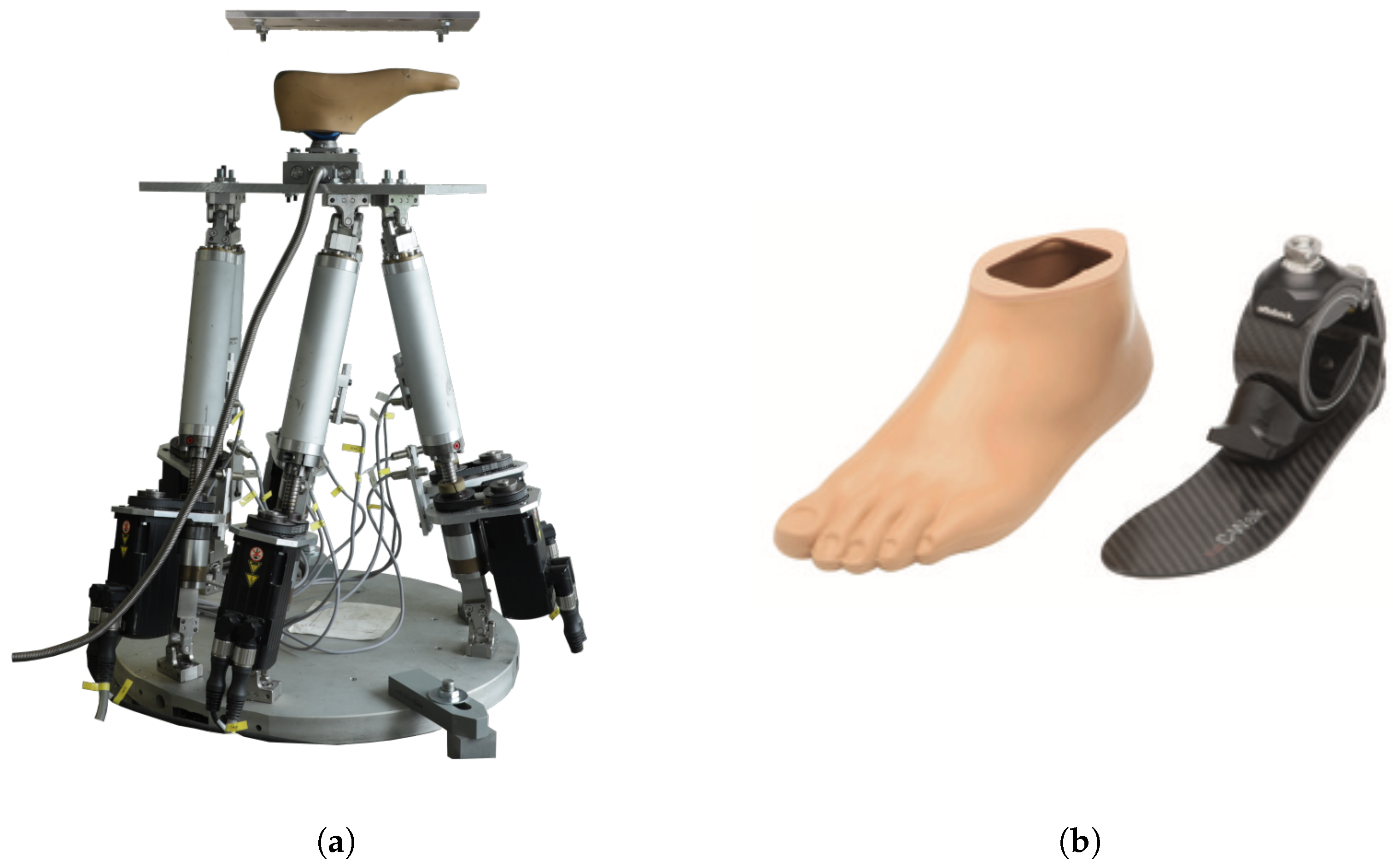
3.2. Transfer System

The transfer system in a HiL test comprises an actuator, a DSP, and an FTS. The actuator used was an in-house built Stewart Platform. Parallel robots have a high load capacity, a high rigidity, and a high positioning accuracy [26]. The Stewart Platform was controlled with a decentralized controller, i.e., each leg was controlled individually. The upper plate of the Stewart Platform has six DoFs (three translations, three rotations). A cascaded control scheme was implemented and a velocity feedforward controller used to improve the actuator agility. Details about the controller implementation can be found in [27].

The implementation of the modeled amputee and the actuator control were performed in MATLAB^®/Simulink^®(Version R2016b, The MathWorks Inc., Natick, MA, USA). In the real-time application, these ran on a MicroLabBox dS1202 from dSPACE, which was used as the DSP. The application was controlled from the host PC via ControlDesk^® (Version 6.0).

The Kistler multicomponent dynamometer (Type 9129AA, Kistler Instrumente GmbH, Sindelfingen, Germany) was used as the FTS [28]. This sensor is built with piezoelectric sensors, which are well suited to measure highly dynamic processes. The experimental setup is visualized in Figure 6a.

3.3. Experimental Part

The prosthetic foot used in the test was the Ottobock 1C40 C-Walk. This is an Energy Storage And Return (ESAR) foot [1]. During the stance phase, the carbon spring stores deformation energy, which is unloaded during take off to propel the body forward. The prosthetic foot is depicted in Figure 6b.

3.4. Parameters

This section summarizes the parameters used to conduct one stride with the presented HiL setup. The parameters are given in

Table 1. Parameters and initial conditions used in the HiL test.

Variable	Value	Variable	Value
$l_{0,\mathrm{L}}$, $l_{0,\mathrm{R}}$	1 m	$l_{0,\mathrm{u}}$	0.84 m
$m_{\mathrm{V}\mathrm{P}\mathrm{P}}$	30 kg	$h_{\mathrm{f}}$	0.16 m
$J_{\mathrm{V}\mathrm{P}\mathrm{P}}$	3 kgm2	$m_{\mathrm{I}\mathrm{F}\mathrm{P}}$	0.005 kg
$k_{\mathrm{L}}$	$5.4\times {10}^3\mathrm{N}/\mathrm{m}$	$k_{\mathrm{u}}$	$1.1\times {10}^3\mathrm{N}/\mathrm{m}$
${\alpha }_0$	${75}^{\circ }$	$d_{\mathrm{u}}$	4.69 $\mathrm{k}\mathrm{g}$/s
$r_{\mathrm{V}\mathrm{P}\mathrm{P}}$	0.25 m	$r_{\mathrm{h}}$	0.1 m
$x_0$	0 m	${\dot{x}}_0$	0.97633 m/s
$y_0$	1.0709 m	${\dot{y}}_0$	0 m/s
${\varphi }_{\mathrm{V}\mathrm{P}\mathrm{P},0}$	0 rad	${\dot{\varphi }}_{\mathrm{V}\mathrm{P}\mathrm{P},0}$	−0.0071 $\mathrm{r}\mathrm{a}\mathrm{d}$/s
Solver	Euler	$\Delta \widehat{T}$	0.0002 s
		$\Delta T$	0.001 s

.

The stability of gait models is highly sensitive to the chosen parameters and initial conditions. Due to several hardware limitations of the Stewart Platform, such as limited work space (due to limited actuator stroke), limited maximum actuator velocity/acceleration, and limited maximum force, a scaled model of the amputee had to be found. Using an optimization algorithm, the model parameters and initial conditions (index ${(·)}_0$) as summarized in the table were found for the VPP model. With this set of parameters, the VPP model was able to walk continuously for >50 steps. However, this parameter set is biomechanically not meaningful, because this would be a very lightweight person on long legs. Additionally, the TD angle was quite steep compared to human walking.

The numerical simulation needed to run with a small sample time such that the simulation was numerically stable. Furthermore, the sample time $\Delta \widehat{T}$ could not be too small because the model still had to be solved in real time. In the preliminary analysis, a sample time of $\Delta \widehat{T}=0.0002\mathrm{s}$ proved successful. Furthermore, the sampling of the interface forces was performed with $\Delta \widehat{T}=0.0002\mathrm{s}$. The actuator control ran with a sample time of $\Delta T=0.001\mathrm{s}$.

4. Experimental Results

With the HiL setup and the parameters presented in Section 3, one stride was performed. The following experimental results reflect the measured data during this GC. The stride begins with the single support phase of the left, intact leg. With the TD of the right, amputated leg, the body weight is shifted to the amputated leg, and the prosthetic foot is loaded. With the TO of the left leg, the right leg takes over the full body weight. Then, the left leg touches down again, and the HiL test is concluded at midstance of the left leg. The goal of this study was to investigate whether an experimental test using the presented HiL setup was feasible and, if so, whether basic gait characteristics according to the VPP model could be replicated in the test.

This test was performed three times, and similar results could be observed in each of the trials. For the sake of clarity, only one of the trials is presented.

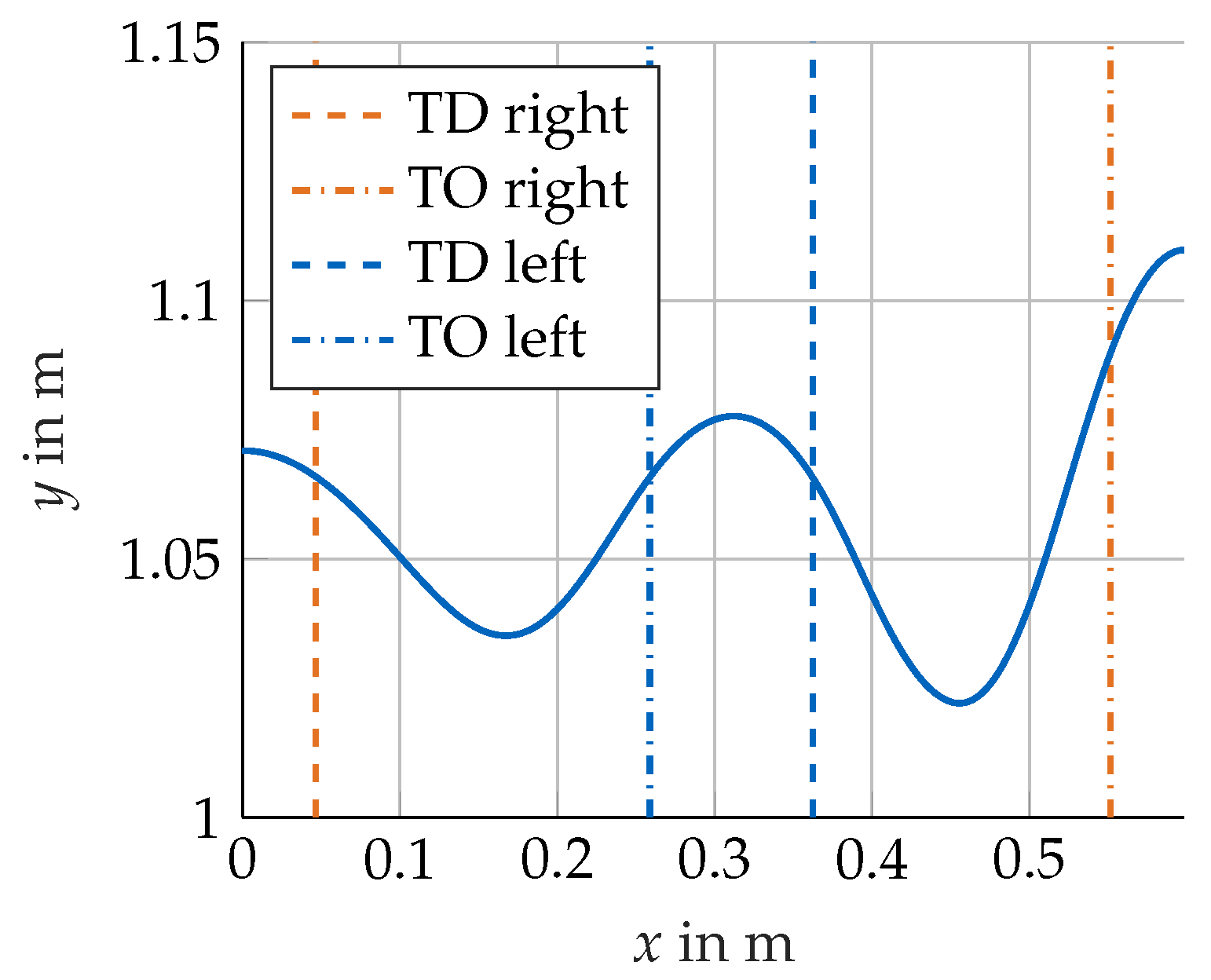
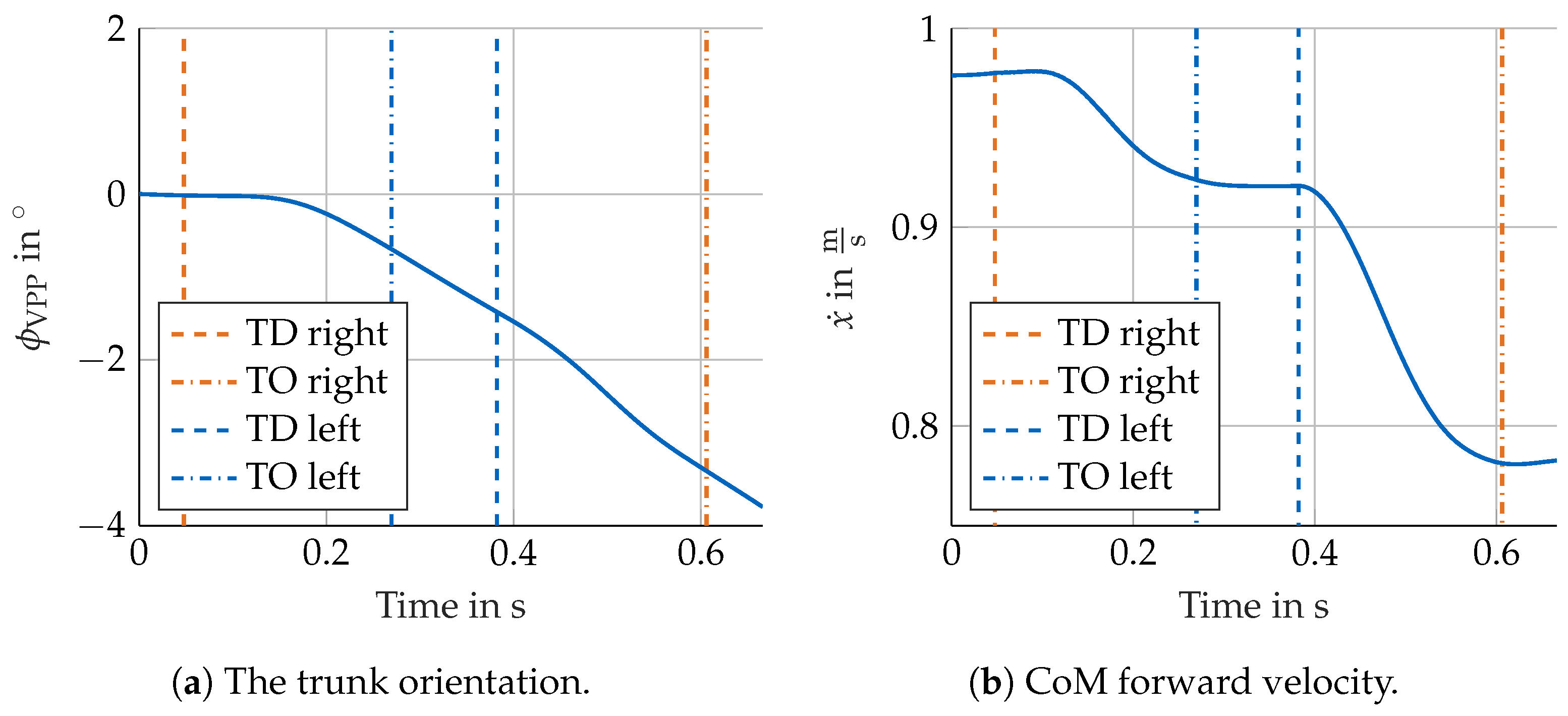
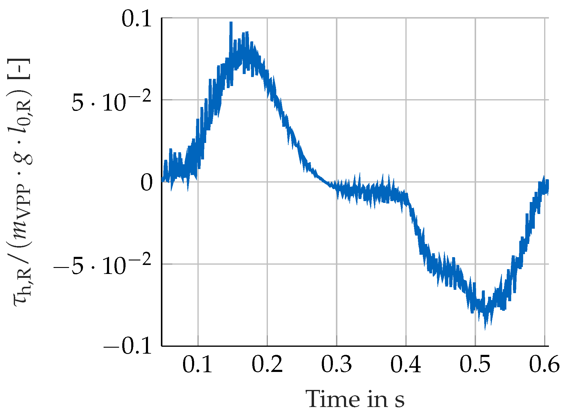
4.1. Results of One Gait Cycle

Firstly, the trajectory of the CoM was analyzed. The results of the HiL test are shown in Figure 7. The CoM trajectory exhibited a sinusoidal shape in y direction. The maxima were when the CoM was above one leg (midstance). For the left left leg, this was at $x=0\mathrm{m}$ and $x\approx 0.6\mathrm{m}$, and right midstance occurred at $x\approx 0.3\mathrm{m}$. The oscillation magnitude was $\approx 0.04\mathrm{m}$, which corresponds well with the observations made in human walking ($0.032\pm 0.008\mathrm{m}$ [14]). In continuous human walking (and also for stable walking models), the motion trajectory oscillates with a constant magnitude. In this HiL test, the magnitude increased, or in other words, the CoM was lifted excessively for $x>0.45\mathrm{m}$. In this phase, the prosthetic foot rolled over the forefoot. Since the ankle joint is not flexible, the CoM needed to be lifted.

Next, the orientation of the trunk was analyzed. The results are visualized in Figure 8a. The figure reveals that the trunk rotated backwards throughout the whole GC. For continuous walking, an oscillations of the trunk about $0{}^{\circ }$ was expected. This suggests that the model is about to fall backwards and that the parameters used for the simulation do not lead to a continuous gait pattern. The duration of the GC was $0.67\mathrm{s}$, which corresponds to the duration of the GC in a pure simulation of the VPP model with the same biomechanical parameters and initial conditions. The proportion of the stance phase of the right leg in the GC was $85\%$. In normal human walking, this is only $60\%$. The single support phase of the right leg was relatively short with $17\%$ of the GC. The reason might lie in the relatively slow forward velocity of the model that was selected to meet the hardware limitations of the Stewart Platform: when humans walk slowly, the stance time, as well as the double-stance phase increase, because the body needs to be balanced more [14].

The modeled amputee, as shown in Figure 8b, initially walked at a speed of $0.98\mathrm{m}/\mathrm{s}$ (the preferred walking speed of able-bodied people is $1.36\mathrm{m}/\mathrm{s}$). During the GC, the forward velocity decreased to $0.78\mathrm{m}/\mathrm{s}$. Together with Figure 8a (backward movement of the trunk, ${\varphi }_{\mathrm{V}\mathrm{P}\mathrm{P}}<0^{\circ }$), this revealed that the model lost energy and could not walk stably with the selected parameters and initial conditions. There are several reasons for this: The initial values of the gait model were found based on an optimization of the VPP model that did not include the CoP shift. Due to this forward shift, the time span where the CoM was behind the foot point (in x direction) was prolonged. Since the CoM decelerated as long as the CoM was behind the foot, the system energy decreased. A further reason why energy was lost is the added damper. The amount of dissipated energy was not compensated. With respect to the system energy, this energy dissipation was small (≈5%). Due to the three-dimensional foot, the CoM was lifted in the second half of the right leg’s stance phase (cf. Figure 7). The conversion of kinetic energy into potential energy is a further reason why the CoM velocity decreased. Furthermore, there was energy lost in the foot impact and by the deformation of the prosthetic foot. Based on these results, one can assume that the model would not be able to complete a second stride and would tip over backwards.

Another important characteristic of human gait is the GRFs, as illustrated in Figure 9a. The GRFs in the vertical direction (${GRF}_{\mathrm{R},y}$) represent the typical m-shape with two maxima and one minimum in between. Similar to observations made in human walking, the maximum values featured a magnitude of approximately $110\%$ of the body weight. The GRFs in anterior/posterior direction (${GRF}_{\mathrm{R},x}$) met the expectations: the absolute value of the maximum forces (≈$50\mathrm{N}$) was lower than $25\%$ of the body weight, and the measured forces changed sign from negative to positive over the course of the stance phase [15]. Hence, the shape of the GRFs was as expected and observed in humans. However, the second hump of the GRFs in y exhibited a steep initial rise, which resembled an impact. The reason for this sharp increase lies in the performance limitations of the Stewart Platform and the high stiffness of the prosthetic foot. The commanded and the real displacement of one leg of the Stewart Platform during this HiL test are visualized in Figure 9b.

When the prosthetic foot rolled over its forefoot, the forces increased, and the VPP model would lift (at $t>0.4\mathrm{s}$). Even though the Stewart Platform was driven at its limits (maximum motor voltage), it was not able to follow the desired motion, and the GRFs increased sharply. In case a more powerful hardware setup is used, this limitation could be circumvented.

Within the implementation of the VPP model, a hip torque was included to stabilize the trunk. The hip torque of the right hip ${\tau }_{\mathrm{h},\mathrm{R}}$ (see Equation (10)) is depicted in Figure 10 normalized over the body weight and leg length. A positive hip torque was seen in the first half of the stance phase, which prevented the trunk from falling forward, and a negative hip torque was applied in the second half to counteract a backward rotation of the torso. This general tendency met the expectations based on human gait analysis [17].

4.2. Discussion

The results revealed that the gait characteristics of the HiL test qualitatively resembled those of the VPP model. This implies that the dynamic interaction between the prosthetic foot and the amputee can be replicated by a HiL setup. Nevertheless, there were some limitations in the current implementation that prevented accurate mimicking of human gait characteristics.

The biomechanical parameters used in this study had to be selected based on several hardware limitations of the Stewart Platform and the suspension frame. These parameters represent a light person ($m_{\mathrm{V}\mathrm{P}\mathrm{P}}=30\mathrm{k}\mathrm{g}$) with long legs ($l_{0,\mathrm{j}}=1\mathrm{m}$) and a relatively steep angle of attack (${\alpha }_0={75}^{\circ }$), which is biomechanically not meaningful. Neither, this test was able to replicate the gait dynamics of amputees observed in gait laboratories (asymmetry, energy consumption, etc.). Nevertheless, this study did not claim to quantitatively emulate a walking amputee, but rather to investigate whether a HiL test of a human wearing a prosthetic foot was feasible.

The VPP model was a good basis to model the amputee for this first proof-of-concept study. In the future, making further adaptations to the implemented VPP model is desirable. For example, the initial conditions should be tuned. Furthermore, the trajectory of how the CoP shifts from the heel to the toes could be implemented based on observations in humans. Furthermore, using more complex models that more realistically model human gait is targeted. A suitable model could be the neuromuscular–skeletal model by Geyer and Herr [29], which includes the foot geometry and models the legs more realistically.

Even though this first HiL test worked in the sense that basic gait characteristics could be replicated, no final conclusion can be drawn whether HiL is a suitable future testing method for prosthetic feet. As next steps, the VPP model can be further tuned (e.g., mass, stiffness, initial conditions) or changes to the prosthetic foot made (mounting, e.g., with different rotations or shifting it forward/backward). With these tests, we wanted to investigate whether changes in the gait dynamics of the modeled amputee were visible. If this were the case, HiL tests could be a meaningful means to understand the dynamic interaction of humans and prosthetic feet better and improve foot prostheses. From these first results, the following requirements for prostheses testing with HiL can be inferred: Powerful hardware is required in order to replicate the dynamic motion. This includes, i.a., a stiff actuator, high computation power, and a stiff suspension frame. Furthermore, the accuracy of the gait characteristics was just as good as the underlying model of the amputee.

5. Summary and Conclusions

This paper provided a proof-of-concept about whether HiL is generally suitable to represent the dynamic interaction of a human with a prosthesis. For that purpose, a HiL setup of a modeled amputee and a prosthetic foot was developed, which performed one stride. The amputee was modeled based on the Virtual Pivot Point (VPP) model. The modifications of the VPP model included (i) the insertion of a mass interface point at the ankle joint, (ii) the insertion of a damper along the leg axis to dampen oscillations of the mass interface point, and (iii) the implementation of a forward shifting center of pressure, which is the point where the ground reaction forces are applied. The results of the HiL test showed the center of mass motion and velocity, the ground reaction forces, and the hip torque of the amputee during one stride. All these quantities qualitatively emulated human gait characteristics well and revealed the potential of HiL to emulate the dynamic interaction between the human and the prosthesis. Differences from the VPP model can be explained by the modifications made to model the amputee and the limited performance of the used Stewart Platform. This work therefore forms the basis for further work and to develop HiL as a test method for prosthetic feet. There are still many research questions to be answered before HiL can be used as a test method. In the future, more complex gait models will be implemented. Additionally, different prosthetic feet will be mounted and the parameters of the human gait model altered to investigate how gait characteristics change. This analysis will help to understand the dynamic interplay between a human and prosthetic feet better.

References

1. Tryggvason, H.; Starker, F.; Lecompte, C.; Jónsdóttir, F. Modeling and simulation in the design process of a prosthetic foot. In Proceedings of the 58th Conference on Simulation and Modelling (SIMS 58), Reykjavik, Iceland, 25–27 September 2017; Linköping Electronic Conference Proceedings. Linköping University Electronic Press: Linköping, Sweden, 2017; pp. 398–405. [Google Scholar] [CrossRef] [Green Version]
2. Kwon, S.; Park, J. Kinesiology-Based Robot Foot Design for Human-Like Walking. Int. J. Adv. Robot. Syst. 2012, 9, 259. [Google Scholar] [CrossRef] [Green Version]
3. Murphy, D. 20—Gait Deviations after Limb Loss. In Fundamentals of Amputation Care and Prosthetics; Demos Medical Publishing: New York, NY, USA, 2013. [Google Scholar]
4. Gailey, R.; Allen, K.; Castles, J.; Kucharik, J.; Roeder, M. Review of secondary physical conditions associated with lower-limb amputation and long-term prosthesis use. J. Rehabil. Res. Dev. 2008, 45, 15–29. [Google Scholar] [CrossRef] [PubMed]
5. International Organization for Standardization. Prosthetics–Structural Testing of Lower-Limb Prostheses–Requirements and Test Methods; Standard; ISO/TC 168 Prosthetics and Orthotics; International Organization for Standardization: Geneva, Switzerland, 2016. [Google Scholar]
6. International Organization for Standardization. Prosthetics–Quantification of Physical Parameters of Ankle Foot Devices and Foot Units; Standard; ISO/TC 168 Prosthetics and Orthotics; International Organization for Standardization: Geneva, Switzerland, 2016. [Google Scholar]
7. Yang, Z. Development of a Gait Simulator for Testing Lower Limb Prostheses. Ph.D. Thesis, University of Bath, Bath, UK, 2020. [Google Scholar]
8. Timmers, N. Simulating Gait with the 3R60 Knee Prosthesis and a Control Moment Gyroscope. Master’s Thesis, TU Delft, Delft, The Netherlands, 2020. [Google Scholar]
9. Windrich, M.; Grimmer, M.; Christ, O.; Rinderknecht, S.; Beckerle, P. Active lower limb prosthetics: A systematic review of design issues and solutions. BioMed. Eng. OnLine 2016, 15, 5–19. [Google Scholar] [CrossRef] [PubMed] [Green Version]
10. Richter, H.; Simon, D.; Smith, W.A.; Samorezov, S. Dynamic modeling, parameter estimation and control of a leg prosthesis test robot. Appl. Math. Model. 2015, 39, 559–573. [Google Scholar] [CrossRef]
11. Marinelli, C. Design, Development and Engineering of a Bench for Testing Lower Limb Prosthesis, with Focus on High-Technological Solutions. Ph.D. Thesis, Politecnico di Milano, Milan, Italy, 2016. [Google Scholar]
12. Predovic, J. Walking Cycle Man. Available online: https://svg-clipart.com/man/YS0etCS-walking-cycle-man-clipart (accessed on 8 May 2012).
13. Millitzer, J.; Mayer, D.; Henke, C.; Jersch, T.; Tamm, C.; Michael, J.; Ranisch, C. Recent Developments in Hardware-in-the-Loop Testing. In Model Validation and Uncertainty Quantification; Barthorpe, R., Ed.; Springer International Publishing: Cham, Switzerland, 2019; Volume 3, pp. 65–73. [Google Scholar]
14. Perry, J.; Burnfield, J.M. Gait Analysis: Normal and Pathological Function, 2nd ed.; SLACK: Thorofare, NJ, USA, 2010. [Google Scholar]
15. Whittle, M.W. Gait Analysis: An Introduction; Butterworth-Heinemann: Oxford, UK, 1991. [Google Scholar]
16. Murphy, D. 19—Normal Human Gait. In Fundamentals of Amputation Care and Prosthetics; Demos Medical Publishing: New York, NY, USA, 2013. [Google Scholar]
17. Winter, D.A. The Biomechanics and Motor Control of Human Gait; University of Waterloo Press: Waterloo, ON, Cananda, 1987. [Google Scholar]
18. Maus, H.M.; Lipfert, S.W.; Gross, M.; Rummel, J.; Seyfarth, A. Upright human gait did not provide a major mechanical challenge for our ancestors. Nat. Commun. 2010, 1, 70. [Google Scholar] [CrossRef] [PubMed] [Green Version]
19. Blickhan, R. The spring-mass model for running and hopping. J. Biomech. 1989, 22, 1217–1227. [Google Scholar] [CrossRef]
20. Maus, H.M. Towards Understanding Human Locomotion. Ph.D. Thesis, Technical University of Ilmenau, Ilmenau, Germany, 2012. [Google Scholar]
21. Vielemeyer, J.; Müller, R.; Staufenberg, N.S.; Renjewski, D.; Abel, R. Ground reaction forces intersect above the center of mass in single support, but not in double support of human walking. J. Biomech. 2021, 120, 110387. [Google Scholar] [CrossRef] [PubMed]
22. Maus, H.M. Stabilisierung des Oberkörpers beim Rennen und Gehen. Diploma Thesis, Friedrich Schiller University Jena, Jena, Germany, 2008. [Google Scholar]
23. Holzberger, F. Vergleich von Gehmodellen des Menschen zur Verwendung in Prothesen-Tests. Semester Thesis, TU München, Munich, Germany, 2020. [Google Scholar]
24. Fan, K. Setting up a Hybrid Substructuring Test for Prosthetic Feet. Master’s Thesis, Technical University of Munich, Munich, Germany, 2020. [Google Scholar]
25. Nolan, K.J.; Yarossi, M.; Mclaughlin, P. Changes in center of pressure displacement with the use of a foot drop stimulator in individuals with stroke. Clin. Biomech. 2015, 30, 755–761. [Google Scholar] [CrossRef] [PubMed]
26. Siciliano, B.; Khatib, O. Springer Handbook of Robotics; Springer: Berlin, Germany, 2016; Chapter 18. [Google Scholar]
27. Insam, C.; Göldeli, M.; Klotz, T.; Rixen, D.J. Comparison of Feedforward Control Schemes for Real-Time Hybrid Substructuring (RTHS). In Dynamic Substructures; Springer International Publishing: Cham, Switzerland, 2021; pp. 1–14. [Google Scholar]
28. Kistler Group. Instruction Manual, Multicomponent Dynamometer Type 9129AA; Kistler Group: Winterthur, Switzerland, 2015. [Google Scholar]
29. Geyer, H.; Herr, H. A muscle-reflex model that encodes principles of legged mechanics produces human walking dynamics and muscle activities. IEEE Trans. Neural Syst. Rehabil. Eng. 2010, 18, 263–273. [Google Scholar] [CrossRef] [PubMed]
Figure 1. To investigate the gait dynamics of an amputee wearing a prosthesis, the application of HiL is proposed. The simulated amputee is coupled with the experimentally tested prosthetic foot. The coupling is achieved by an actuator (Stewart Platform in the figure) and a force–torque sensor. The prosthetic foot is moved by the actuator according to the calculations of the simulated amputee. The picture of the amputee is adapted from [12], license CC BY 4.0.
Applsci 11 09492 g001
Figure 2. To couple the numerical (in blue) and experimental part (in green), a transfer system (in orange) is used. The transfer system consists of a controlled actuator, an FTS, and a DSP. The DSP is not visualized in the figure.
Applsci 11 09492 g002
Figure 3. The hip torque τ V P P , j generates a force F τ , j orthogonal to the leg axis that redirects the GRFs G R F j into the VPP. γ V P P , j represents the angle between the leg and the connection between the foot point x F P , j and the VPP ( x V P P , y V P P ) . The orientation of the trunk is defined by ϕ V P P . For the sake of clarity, only one leg ( j = { L , R } ) is shown here. Figure adapted from [23] (reprinted with permission from [23], 2020 Holzberger).
Applsci 11 09492 g003
Figure 4. Model of the amputee based on the VPP model. The right leg is cut, and a point mass m I F P is added to serve as an interface point between the simulation and experimental system. A damper between the hip and point mass is added to reduce oscillations. The resting leg length of the remaining upper part of the right leg is l 0 , u . At the interface point ( x I F P , y I F P ), the measured forces/torque F int act on the model. Figure adapted from [23] (reprinted with permission from [23], 2020 Holzberger).
Applsci 11 09492 g004
Figure 5. The implementation of the VPP model assumes that the GRFs act at the CoP. The figures were inspired by [23] (reprinted with permission from [23], 2020 Holzberger). (a) The implementation assumes a linear shift of the CoP from the heel to the toes depending on the leg angle α R . (b) The measured forces F int result from the GRFs. Inertial forces and gravitational forces are neglected.
Applsci 11 09492 g005
Figure 6. The transfer system and the experimental part are depicted. (a) The experimental setup consists of the prosthetic foot, the FTS, and the Stewart Platform. (b) The C-Walk foot 1C40 by Ottobock with silicone cosmesis (© by Ottobock).
Applsci 11 09492 g006
Figure 7. CoM trajectory of the modeled amputee during one GC in the HiL test.
Applsci 11 09492 g007
Figure 8. The CoM trajectory, as well as the trunk orientation of the modeled amputee during the HiL test of one GC.
Applsci 11 09492 g008
Figure 9. Measurement data during the HiL test. (a) The GRFs in the x and y direction during the stance phase of the right leg. The black dashed line indicates the body weight. (b) The desired and real displacement of the Stewart Platform’s Leg 1 are shown. Leg 1 undergoes the largest motion command of all six legs.
Applsci 11 09492 g009
Figure 10. Total hip torque normalized over body weight and leg length during the stance phase of the right leg.
Applsci 11 09492 g010