A Computational Study on Magnetic Nanoparticles Hyperthermia of Ellipsoidal Tumors

Abstract

The modelling of magnetic hyperthermia using nanoparticles of ellipsoid tumor shapes has not been studied adequately. To fill this gap, a computational study has been carried out to determine two key treatment parameters: the therapeutic temperature distribution and the extent of thermal damage. Prolate and oblate spheroidal tumors, of various aspect ratios, surrounded by a large healthy tissue region are assumed. Tissue temperatures are determined from the solution of Pennes’ bio-heat transfer equation. The mortality of the tissues is determined by the Arrhenius kinetic model. The computational model is successfully verified against a closed-form solution for a perfectly spherical tumor. The therapeutic temperature and the thermal damage in the tumor center decrease as the aspect ratio increases and it is insensitive to whether tumors of the same aspect ratio are oblate or prolate spheroids. The necrotic tumor area is affected by the tumor prolateness and oblateness. Good comparison is obtained of the present model with three sets of experimental measurements taken from the literature, for animal tumors exhibiting ellipsoid-like geometry. The computational model enables the determination of the therapeutic temperature and tissue thermal damage for magnetic hyperthermia of ellipsoidal tumors. It can be easily reproduced for various treatment scenarios and may be useful for an effective treatment planning of ellipsoidal tumor geometries.

1. Introduction

The most well-known techniques for cancer treatment are chemotherapy, radiation, immunotherapy and targeted therapy [1,2,3]. These treatments suffer from various severe side effects such as hair loss, nausea, infertility, nerve damage and general discomfort to the patient [3].

Hyperthermia is a widely studied treatment with a broad spectrum of applications ranging from cardiac ablation [4,5] to arterial low-density lipoprotein (LDL) deposition [6,7] to drug delivery enhancement [8,9] and thermal ablation of tumors under microwaves [10,11,12] and/or with magnetic nanoparticles (MNPs) [13,14,15].

The hyperthermia of tumors is regarded as a viable treatment provided that the tumor locations are known and have not metastasized or when it is difficult to surgically remove the tumor, such as in liver cancer [16]. The ultimate treatment goal is to raise the tumor temperature above the physiological temperature for a certain time and to damage the malignant cells through several mechanisms such as protein denaturation, apoptosis and necrosis [17], without significantly affecting the surrounding healthy tissue. In mild hyperthermia the tumor temperature usually ranges between 40–45 °C and typically above 50 °C for ablation therapy [18,19,20,21,22].

MNPs have a broad spectrum of applications such as heat exchangers, solar collectors and separation of heavy metals from water [23,24,25]. Hyperthermia using MNPs (magnetic hyperthermia) has received increased attention due to its ability to deliver adequate heating power to several types of tumors [26]. The therapy involves the administration of MNPs, usually in the form of colloidal suspensions, intravenously or directly into the tumor, and subsequently exposing the MNPs loaded tumor to an external alternating magnetic field (AMF) [27,28]. From clinical trials, it has been shown that the product of the magnetic field amplitude and field frequency must be kept below the value of approximately 4.85 × 10⁸ A∙m⁻¹∙s⁻¹ for safety purposes [29,30]. For intravenous injection, the magnetic field may also facilitate the nanoparticles magnetic guidance towards the desired location [31,32]. Due to the AMF, the injected nanoparticles generate heat via mainly two mechanisms, usually referred to as Néelian and Brownian relaxations. Based on this, Rosenzweig [33] developed a theoretical heat generation model that takes into account the magnetic properties of the nanoparticles as well as properties associated with the applied magnetic field. The efficiency of MNPs to convert electromagnetic energy into heat may be quantified experimentally, usually by specific loss power (SLP), also referred to as specific absorption rate (SAR) [15,34]. The most common types of MNPs used to date are superparamagnetic iron oxide nanoparticles (SPIONs) such as magnetite Fe₃O₄ and maghemite γ-Fe₂O₃ [35,36,37], due to their biocompatibility [38] upon injection in human tissues. Several other nanoparticle types have also been reported, such as metallic alloys [39,40] and carbon nanotubes [41]. The distribution of the nanoparticles reaching the tumor may generally vary from approximately uniform distributions throughout the whole tumor to fully localized ones inside specific tumor regions as observed from real tumor sections [42,43]. The distributions depend on several factors such as injection parameters, the tumor’s physiological and mechanical properties, and the physicochemical properties of the nanoparticles [44,45,46].

According to several studies [47,48,49], modeling the magnetic hyperthermia plays a seminal role in the treatment. Determination of the therapeutic temperature profile and the treatment duration are key parameters frequently taken into consideration during the treatment procedure. These can be predicted usually by solving the Pennes bio-heat transfer equation [50], but other models have also been proposed to predict heating effects such as, for instance, porous media based models [51,52]. Treatment temperature and duration may also affect the mortality of the malignant or healthy cells, which can be evaluated by the Arrhenius formulation description; the treatment thermal dose usually evaluated by the Cumulative Equivalent Minutes is at the 43 °C (CEM43) parameter [21,53,54,55,56,57] or the temperature threshold method [58,59]. Other cell death models have been also developed [60,61].

The most frequently assumed tumor shape, in numerous earlier modeling studies, is a perfect sphere. Such an ideal geometry allows for derivation of analytical expressions for the therapeutic temperature profile [62,63,64,65,66,67,68,69]. Also, for spherical tumors, numerical models have been formulated using the finite element, finite volume and Lattice Boltzmann methods [70,71,72,73,74,75,76,77,78,79]. However, tumor shapes usually depart from the perfect sphericity assumption. Elongated shapes, reminiscent of geometric ellipsoids, are frequently encountered. According to Mills et al. [80] and Kulwanto et al. [81], in vitro experiments have shown that the studied tumors have grown into highly elongated ellipsoidal-like shapes. Similar elongated shapes have also been reported for primary breast carcinoma [82], primary gastric gastrointestinal stromal tumors [83] and glioblastoma related tumors [84]. In fact, in the last three studies relating to overall survival in patients, the tumor volume was calculated by the shape of an ellipsoid. Relevant to magnetic hyperthermia using nanoparticles, several in vivo experimental investigations in rodents show histological cross-sections of subcutaneous and deep-seated tumors that have grown into ellipsoidal-shaped geometries with mild to high aspect ratios [85,86,87,88,89,90,91]. In these studies, the tumor volume was estimated based on the geometric shape of an ellipsoid.

A few researchers have developed some computational models assuming ellipsoid tumor geometry. Pierce et al. [92] report in vivo and 3D computational results of temperature distribution and cell damage of adenocarcinoma subcutaneous tumors in the fore-shoulders of female mice. The shape of the tumors was approximated by an ellipsoid. Rodrigues et al. [93] studied the magnetic nanoparticle hyperthermia of a subcutaneous sarcoma tumor both experimentally and computationally. The shape of the tumor was also approximated by an ellipsoidal shape. Kandala et al. [94] proposed a computational model for the utilization of power modulation for magnetic nanoparticle hyperthermia of elliptic (2D) and ellipsoidal (3D) tumors. In the above-mentioned studies, the aspect ratio of the ellipsoid tumors was fixed.

Egolf et al. [95] developed an analytical model for the transient temperature evolution in three tumor shapes of equal volume: a perfect spherical, a prolate spheroid with an aspect ratio of approximately three and an oblate spheroid with an aspect ratio of eight. Spatial temperature distributions in the tumor and the surrounding healthy tissue were neglected. Their results show that the uniform temperature in the spherical tumor was higher than in the prolate spheroid tumor and much higher than the oblate spheroid tumor. Tehrani et al. [96] studied numerically oblate and prolate spheroid tumors of equal volumes for the treatment of microwave ablation using a coaxial antenna. In their work the aspect ratio of the ellipsoids varied from one to five. Their results show that the aspect ratio has a significant effect on the extent of the ablation zone in the tumor.

The objective of the present investigation is to provide a systematic study for magnetic nanoparticles hyperthermia of ellipsoidal tumors of various aspect ratios and to compare the results of the numerical predictions to experimental data. The tumors are modeled as prolate and oblate spheroids of equal volumes.

2. Materials and Methods

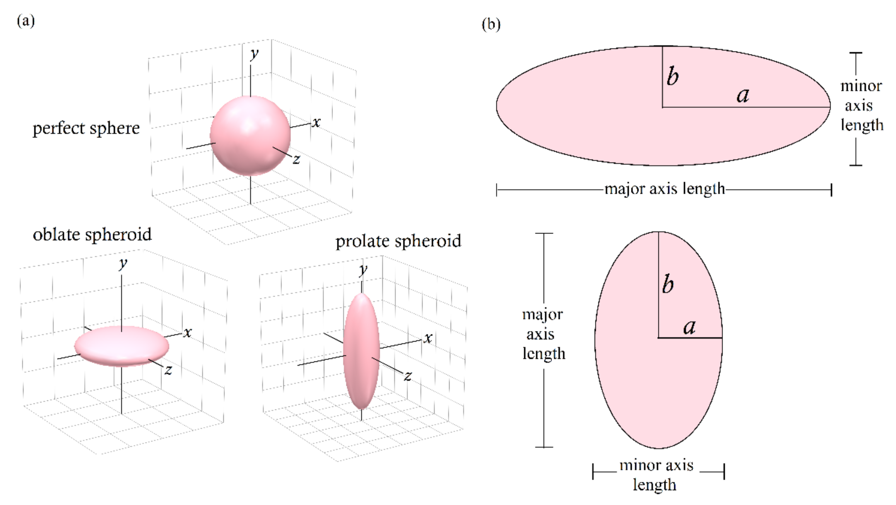
2.1. Geometrical Description

The general equation of an ellipsoid is given by [97]:

$$\frac{x^2}{a^2}+\frac{y^2}{b^2}+\frac{z^2}{c^2}=1$$

(1)

where a, b and c are the lengths of the principal semi-axes. For the case of all lengths equal a = s = c = R, Equation (1) describes a perfect sphere with radius R. In the present work we are interested for ellipsoids with a = c (symmetric around the y axis), while perfect spherical tumors constitute only a limit-case scenario. Such shapes are usually referred to as ellipsoids by revolution. Here, the y-axis is set as the axis of revolution.

Two basic cases may be distinguished:

(i)

oblate spheroids with semi-axis a > b

(ii)

prolate spheroids with semi-axis a < b

as shown in Figure 1.

In addition, we define the aspect ratio AR for the generated ellipsoids using the following notation [96]:

$$\mathrm{AR}=\frac{\mathrm{major}\mathrm{axis}\mathrm{length}}{\mathrm{minor}\mathrm{axis}\mathrm{length}}$$

(2)

Increasing AR leads to ellipsoidal tumors with more elongated shapes. The surface S of the ellipsoids is expressed via the following formulation [98]:

$$S=2\mathsf{\pi }{a}^2\left[1+\left\{\begin{array}{ccc}\frac{b}{ae}\arcsin e ,& e^2=1-{\left(\frac{a}{b}\right)}^2 ,& b>a \left(\mathrm{prolate}\right)\\ & & \\ \frac{b^2}{a^{2}e}\mathrm{arctanh}e ,& e^2=1-{\left(\frac{b}{a}\right)}^2 , & b<a \left(\mathrm{oblate}\right)\end{array}\right\}\right]$$

(3)

where e is the eccentricity of the ellipsoid. The volume of the ellipsoids is given by [95]:

$$V=\frac{4}{3}\mathsf{\pi }{a}^{2}b$$

(4)

All the generated ellipsoidal tumors are set to have equal volumes.

The dimensions of the ellipsoid tumors used in this work are shown in

Table 1. Dimensions of the ellipsoidal tumors studied.

Prolate Tumors
Aspect ratio (AR)	a (mm)	b (mm)
2	7.93	15.87
4	6.29	25.19
8	5.0	40.0
Oblate Tumors
Aspect ratio (AR)	a (mm)	b (mm)
1	10.0	10.0
2	12.5	6.29
4	15.87	3.96
8	20.0	2.50

. The tumor geometries are taken to have the same volume, as calculated from Equation (4). The range of the selected tumor dimensions are within the range of earlier works [80,86,95,96]. It is also assumed that the ellipsoidal tumors are surrounded by healthy tissue of spherical geometry, as shown in Figure 2. The region of the healthy tissue is assumed to be significantly larger than the tumor. In particular, the radius of the healthy tissue R_h is taken approximately eight times larger than the semi-major axis of the tumor with the highest aspect ratio. Due to the rotational symmetry of the geometries, the present thermal problem can be solved as an axisymmetric problem instead of a 3D one, which substantially decreases the computational cost of the numerical simulations [99].

For the discretization of the computational domains, we used a combination of regular and unstructured meshes consisting of triangular cells. All meshes were constructed using GMSH software [100]. The unstructured mesh is used to discretize the tumor region as well as a healthy tissue layer around the tumor. We followed this approach to better capture the surface geometry of the tumors with high aspect ratios (e.g., AR = 8). Two sample meshes for AR = 2 are shown in Figure 3.

2.2. Bio-Heat Transfer Analysis

Bio-heat transfer between the ellipsoidal tumor and the surrounding healthy tissue is expressed by the thermal energy balance for perfused tissues described by the Pennes bio-heat equation [93,94]:

$${\rho }_n{c}_n\frac{\partial T\left(x,y,t\right)}{\partial t}=k_n{\nabla }^{2}T\left(x,y,t\right)-{\rho }_{\mathrm{b}}{c}_{\mathrm{b}}{w}_{\mathrm{b},n}\left[T\left(x,y,t\right)-T_{\mathrm{b}}\right]+Q_{\mathrm{met}.,n}+Q_{\mathrm{s}}$$

(5)

where the subscript n stands for the tissue under consideration (n = 1 for tumor and n = 2 for healthy tissue) and the subscript b corresponds to blood properties. Also, ρ_n and ρ_b denote the densities of the tissues and the blood respectively, c_n and c_b are the corresponding heat capacities, T(x,y,t) is the local tissue temperature, k_n is the tissue thermal conductivity, w_b is the blood perfusion rate, and T_b = 37 °C is the blood temperature.

The left–hand side term in Equation (5) expresses the time rate of change of internal energy per unit volume. Τhe first term on the right-hand side of Equation (5) represents the heat conduction in the tissue. The second term represents an additional change in the internal energy per unit volume associated with blood perfusion in tissue, assuming that the rate of heat transfer between tissue and blood is proportional to the blood perfusion rate and the difference between the local tissue temperature and the blood temperature, as suggested in [65]. In addition, Q_met,n is the internal heat generation rate per unit volume associated with the metabolic heat production. Finally, Q_s is the power dissipation density by the MNPs. It is assumed no leakage of MNPs to the surrounding healthy tissue. Therefore, Q_s is only applied to the cancerous region filled with the MNPs, similarly to several earlier investigations, e.g., [15,67,69,92]. Following the assumptions by [42,44,92,95,101], a uniform distribution of nanoparticles is assumed. The temperature of the surface of the healthy tissue region (see Figure 2), which is far away the tumor surface as explained in the previous section, is set to T_s = T_b [69,75]. For the initial temperature condition we set T(x,y,t = 0) = T_b. A symmetry (zero heat flux) boundary condition is applied on the x- and y-axes (line OA and line OB respectively in Figure 2). Also, heat flux and temperature continuity are considered on the tumor-healthy tissue interface as follows [12,93]:

$$k_n{\left(\frac{\partial T}{\partial n}\right)}_n=k_{n+1}{\left(\frac{\partial T}{\partial n}\right)}_{n+1}$$

(6)

$$T_n=T_{n+1}$$

(7)

where n is the direction vector perpendicular to the tumor surface. To carry out numerical simulations for the different AR cases, typical tissue thermophysical values (for example prostate tissue) are chosen from earlier works [36,63,67,71,94] and shown in

Table 2. Physical properties of the tissues [36,63,67,71,94].

Tissue	ρ (kg/m3)	c (J/kg∙K)	k (W/m∙K)	wb (s−1)	Qmet (W/m3)
Tumor	1045	3760	0.5	1.3 × 10−3	540
Healthy tissue	1045	3760	0.5	1.3 × 10−3	540
Blood	1060	3770	–	–	–

. Note that we have assumed that the perfusion rate is independent from region and temperature [31,58]. We have also assumed that the thermophysical properties of the tumor and the healthy tissue are the same, based on earlier works [36,67,71,94] For a complete mathematical formulation of heat transfer in a solid body and the implementation of “internal heat generation” terms within a numerical setting, the interested reader can be referred to [102].

Equation (5) is solved numerically using the open-source software OpenFOAM [99,103] which is based on the finite volume method (FVM). The equations are solved utilizing a preconditioned bi-conjugate gradient (PBiCG) with diagonal incomplete-LU (DILU) preconditioning [104]. The tolerance was set to 10⁻⁸. To speed up the simulations we ran them in parallel mode on a system of distributed processors by geometric domain and associated field decomposition, as described in [105].

2.3. Heat Generation by the Magnetic Nanoparticles

As explained in the work by Miaskowski and Sawicki [49], the superparamagnetic heating phenomenon is the base of magnetic nanoparticles hyperthermia. Rosensweig [33] formulated a theoretical model for the heating of colloidal magnetic fluid (ferrofluid) due to application of an AFM. In his work, the power dissipation density (in W/m³) from a monodispersed magnetic fluid filled with superparamagnetic particles subjected to an alternating magnetic field [15] is given by:

$$Q_{\mathrm{s}}={\mathsf{\pi }\mathsf{\mu }}_0{\chi }_0{H}_0{}^{2}f\frac{2\mathsf{\pi }f\tau }{1+{\left(2\mathsf{\pi }f\tau \right)}^2}$$

(8)

where μ₀ = 4$\mathsf{\pi }$ × 10⁻⁷ H∙m⁻¹ is the vacuum magnetic permeability, f is the frequency of the magnetic field with magnetic field intensity H₀ (A∙m⁻¹), χ₀ corresponds to the magnetic susceptibility of the magnetic fluid defined by

$${\chi }_0={\chi }_{\mathrm{i}}\left(\coth \xi -\frac{1}{\xi }\right)$$

(9)

where χ_i the initial susceptibility given by

$${\chi }_{\mathrm{i}}=\frac{{\mathsf{\mu }}_{0 }\phi {{\rm M}}_{\mathrm{d}}{}^2 V_m}{3{\mathrm{k}}_{\mathrm{B}}T}$$

(10)

and

$$\xi =\frac{{\mathsf{\mu }}_0 M_{\mathrm{d} }{H}_0 V_{\mathrm{m}}}{3{\mathrm{k}}_{\mathrm{B}}T}$$

(11)

with M_d the domain magnetization of a suspended particle, V_m = 4/3R³ is the magnetic volume for a nanoparticle of radius R, k_B = 1.381 × 10⁻²³ J∙K⁻¹ is the Boltzmann constant and T is the absolute temperature. In Equation (10), φ is the solid volume fraction of the nanoparticles. The power dissipation is accomplished via two physical processes, the Néel and Brownian relaxation. Because these processes take place in parallel, the effective relaxation time in Equation (5) is given by

$$\frac{1}{\tau }=\frac{1}{{\tau }_{\mathrm{B}}}+\frac{1}{{\tau }_{\mathrm{N}}}$$

(12)

where τ_B the Brownian characteristic relaxation time

$${\tau }_{\mathrm{B}}=\frac{3\eta V_{\mathrm{H}}}{{\mathrm{k}}_{\mathrm{B}}T}$$

(13)

with η the viscosity of the matrix fluid and V_H is taken as the hydrodynamic volume of the nanoparticle related to V_m as V_H = (1 + δ/R)³V_m where δ is the thickness of a sorbed surfactant layer (δ = 2 nm according to Rosensweig [33]). In Equation (13) τ_N is the Néel characteristic relaxation time given by [15]:

$${\tau }_{\mathrm{N}}=\frac{\sqrt{\mathsf{\pi }}}{2}{\tau }_0\frac{\exp \left(\Gamma \right)}{{\Gamma }^{1/2}}, \Gamma =\frac{\mathcal{K}{V}_{\mathrm{m}}}{{\mathrm{k}}_{\mathrm{B}}T}$$

(14)

where τ₀ ≈ 10⁻⁹ s is an attempt time [15,49] and $𝒦$ is the anisotropy constant (J/m).

2.4. Tissue Thermal Damage

In the present work, the extent of the tissue thermal damage is determined with the Arrhenius kinetic model, which has been used in several studies, e.g., [21,76,106]. This model was originally proposed by Henriques and Moritz [107,108], where the tissue damage is expressed via a dimensionless damage parameter Ω, given by:

$$\Omega =\ln \left\{\frac{C\left(0\right)}{C\left(\tau \right)}\right\}=\underset{0}{\overset{\tau }{{\displaystyle \int }}}A\exp \left[\frac{-E_{\mathrm{a}}}{\mathrm{R}T\left(x,y,t\right)}\right]\mathrm{d}t$$

(15)

where τ is treatment duration, C(0) is the original concentration of the tissue constituent, C(τ) the undamaged tissue constituent at the end of treatment heating, A the frequency factor (s⁻¹), E_a the activation energy (J∙mol⁻¹) and R the gas constant. The temperature T(x,y,t) in Equation (15) is in Kelvin. Ω = 1 means that the damage process is 63.2% complete [21,54] and the tissue may be assumed to be irreversibly damaged [54,106]. The values of the frequency factor and activation energy depend upon the cell line. For the computational results of the present investigation, the constituent cells of the tissue are assumed to be the AT1 subline of Dunning R3327 rat prostate cells with the corresponding values obtained from earlier works [76,92], namely: A = 2.99 × 10³⁷ s⁻¹ and E_a = 244.8 kJ∙mol⁻¹.

2.5. Mesh and Timestep Sensitivity Analysis

A mesh sensitivity analysis was carried out to determine the size of the mesh. The computational sample meshes are shown in

Table 3. Mesh sensitivity analysis results.

Mesh Number	Number of Cells	Temperature Location 2 mm above Tumor Center (°C)
1	9500	41.581
2	15,740	41.852
3	32,781	41.911
4	57,468	41.915

. The mesh sensitivity was performed on an oblate spheroidal tumor with AR = 8. The quantity for which the analysis was performed is the tumor temperature at a distance 2 mm above the tumor geometric center that lies on the y-axis (see Figure 2) after 30 min of treatment. The simulation results in Table 3 show that increasing the mesh size and the temperature on the above-mentioned location generally increases. However, a closer look at the values shows that from mesh 3 to mesh 4 the temperature values change only on the third decimal, which means that temperature change between these two meshes is about 0.01%. Since this change is very small, mesh 3 is selected for the numerical simulations. Furthermore, the timestep in the present work is set to 1 s. Simulation runs with a smaller time step were also performed, namely 0.1 s, which resulted in no significant difference (<0.001%) in the solution.

Moreover, the treatment temperature behavior of the computational model is verified with the closed-form transient solution proposed by Liangruksa et al. [67] for a tumor with AR = 1 (perfect sphere). In their work the solution is given in a dimensionless form (Equations (16) and (17) in [67]). Our computational results are in excellent agreement with the closed-form solution, as shown in Figure 4.

3. Computational Results and Discussion

Magnetite (Fe₃O₄) nanoparticles are selected as heat mediators assuming typical magnetic properties, as shown in

Table 4. Magnetic nanoparticles and magnetic field parameters [33,36,47,49,63].

Parameter	Value
Md (kA∙m−1)	446
$𝒦$ (kJ∙m−3)	41
ρnano (kg∙m−3)	5180
R (nm)	9.5
η (Pa∙s)	6.53 × 10−4
φ	4.8 × 10−4
f (kHz)	220
H0 (A∙m−1)	6800

. The magnetic field properties are also presented in Table 4. Note that for the selected H₀ and f values we find H₀ f = 1.496 × 10⁹ A∙m⁻¹∙s⁻¹, which falls between the limits of Atkinson-Brezovich (4.85 × 10⁸ A∙m⁻¹∙s⁻¹) and Dutz-Hergt (5 × 10⁹ A∙m⁻¹∙s⁻¹) criterions [29,30]. Also, the nanoparticles volume fraction we used is low. Therefore, the effective tumor parameters of MNPs-saturated tissue are nearly identical to tumor parameters without nanoparticles that are used in the model. By substituting these parameters in Equation (8) we find Q_s = 1.91 × 10⁵ W/m³, which is within the range of earlier publications [63,65,68].

The computational results are carried out for a 30 min treatment, since in magnetic hyperthermia it is desirable to have a treatment duration as short as possible for safety purposes [76,109]. The duration the AMF is switched on and heats the nanoparticles is assumed to be 22 min [76]. After that time and for the remaining eight minutes of the treatment, the magnetic field is off and stops heating.

To gain an initial understanding of the tissue temperature distribution, in Figure 5 the temperature field is presented for a region near oblate tumors after 22 min of treatment at various AR values. Note that all tumor shapes have the same volume. In all cases the maximum treatment temperature is observed at the tumor center. As the aspect ratio AR increases, this maximum temperature decreases. This is also the case for the temperature on other regions inside the tumor. A similar behavior is observed for the prolate spheroidal tumors as shown in Figure 6. This behavior is consistent with the results of our earlier preliminary work [99]. Note that the tissue and nanoparticle parameters used in [99] are different than the ones used in the present work. Moreover, the bio-heat equation in [99] was solved under a steady state condition. In the current investigation we have used the more realistic temperature time dependent approach which further allows us to determine the extent of the tissue thermal damage with the Arrhenius thermal damage model.

Figure 7 shows time-dependent temperature profiles at the tumor center for all the considered shapes. The AR value appears to have a significant effect on the tumor temperature evolution. At very initial times the temperature in the center increases rapidly and it is relatively independent of the aspect ratio and whether the tumor is an oblate or prolate spheroid. However, at intermediate times, the temperature becomes significantly dependent on the aspect ratio and it remains nearly insensitive to prolate or oblate spheroid shapes of the same AR. For instance, for AR = 1 after 22 min of treatment, the temperature is 46.62 °C, while for AR = 8 the maximum temperature is approximately 3.5 °C less for both prolate and oblate spheroidal tumors.

The above treatment temperature trends could be explained in terms of the surface area of the tumors. From Equation (3), increasing the AR-value of an ellipsoid tumor leads to an increase of the surface area. For instance, for an oblate tumor with AR = 8 the surface area is approximately twice the surface area of a perfectly spherical tumor of the same volume and for a prolate tumor of AR = 8 it is approximately 1.5 times. Since the available surface area increases, the heat transfer from the nanoparticle-saturated tumor to the cooler healthy tissue increases, leading to a drop of the tumor temperature.

Figure 8 shows the temperature values at two representative tumor surface probe locations as shown in Figure 8a. Observation point P1 is fixed on the tumor surface at the semi-minor axis and P2 fixed on the tumor surface at the semi-major axis. For a tumor with AR = 1, both probes give exactly the same temperature, as shown in Figure 8b. Of course, this is due to the perfect spherical symmetry for this tumor and has been shown by several other works. However, as shown in Figure 8c for a prolate and an oblate tumor with AR = 2, the treatment temperature as a function of time, at P1 and P2, differs significantly. While at the start of the treatment the temperature rises rapidly in a similar manner at both probe locations, after a relatively short time the temperature history at P1 is substantially higher than the temperature at P2. For the oblate tumor, after 22 min of treatment, the temperature at P1 is approximately 2 °C higher than the temperature at P2. A similar temperature difference is observed at the corresponding locations for a prolate spheroidal tumor of the same aspect ratio, but with lower treatment temperature values than the oblate. It should be also noted that for the oblate spheroid the temperature at P1 is higher than the temperature at the corresponding location of a perfectly spherical tumor (AR = 1), as compared to Figure 8b. For tumors with AR = 4 (see Figure 8d) the temperature difference between the two probe locations, after 22 min of treatment, increases to approximately 3 °C (for both oblate and prolate shapes), which is also in the case of tumors with an AR of 8 (see Figure 8e). As expected, due to the larger available surface for heat transfer, the temperatures for the case of AR = 8 are lower than for tumors with an AR of 4.

Once the treatment temperature of the proposed model is determined, the degree of thermal damage in the tumor and healthy tissue can be calculated using the Arrhenius kinetic model [21]. The maximum treatment temperature profiles as a function of treatment time presented in the previous figures can be used to evaluate the degree of thermal damage in the tumor center.

The thermal damage at the tumor center as a function of treatment time is shown in Figure 9. At the beginning of the treatment, the thermal damage of the malignant tissue at the tumor center is low and relatively unaffected by the tumor aspect ratio and whether it is a prolate or oblate spheroid. As the treatment time progresses, the highest thermal damage is observed in the tumors with AR = 1 and the lowest for tumors with AR = 8. For example, at 20 min of treatment the Arrhenius damage index is Ω ≈ 2.75 for AR = 1 and Ω ≈ 1 for AR = 8. The thermal damage evolution in the tumor center is generally independent of the tumor prolateness or oblateness, but it is strongly affected by the aspect ratio. Also, after approximately 22 min of procedure, Ω appears to be relatively stable for each aspect ratio. If we select the frequently quoted Ω = 1 threshold value above, which has a relatively high chance of causing irreversible damage the malignant tissue, we find that for AR = 1 this value is reached after approximately 10 min. of treatment. However, for AR = 8, more than 20 min of treatment are required to reach the Ω = 1 threshold value, and shorter times are required for tumors with smaller AR values.

Figure 10 shows the Arrhenius integral Ω in the tumor for three representative geometries. Figure 10a is for AR = 1, Figure 10b for a prolate tumor with AR = 2 and in Figure 10c for an oblate one with AR = 2. For each case, the thermal damage in the central tumor region is higher than regions near the tumor surface, which is the direct result of the temperature distribution (see Figure 5 and Figure 6). To determine the extent of the damaged region in the ellipsoidal tumors, the frequently quoted Ω = 1 criterion is used as carried out by Eltejaei et al. [106] and Andreozzi et al. [110]. In these studies, the boundary between the necrotic tumor area (Ω > 1) and the undamaged tumor region (Ω < 1) was determined using the Ω = 1 iso-contour. If we follow this approach in the sample tumor cases shown in Figure 10, we find that the location of this boundary is significantly affected by the aspect ratio and by whether the tumor is a prolate or oblate spheroid. Interestingly, for an oblate tumor of AR = 2, a small portion of the surrounding healthy tissue may necrose, which is not the case for a prolate tumor of the same aspect ratio.

4. Comparison with Experiments

In the present section, the computational model is compared with three sets of experimental measurements by different researchers.

The first comparison is with the experimental measurements by Hamaguchi et al. [86]. In their work, the tumor was a squamous cell carcinoma on the cervical lymph node of female Japanese white rabbits. According to [86], the ratio of the volume of the cancerous lymph node to that of normal lymph nodes was approximately 11 (cancerous lymph node volume 1161 ± 276.4 mm³, normal lymph node volume 105.6 ± 43.37 mm³). Twenty days after tumor transplantation, magnetite nanoparticles, of average core magnetite size D = 10 nm, were injected from the rabbit tongue. The average nanoparticle uptake from the cancerous lymph was approximately 4 mg ± 1 mg. For the hyperthermia treatment, a transistor inverter was used with frequency 118 kHz and magnetic field strength of 384 Oe or 30.6 kA/m. From a histological section of the swollen lymph, we approximated the tumor shape with a prolate spheroid that we fitted on top of the tumor. Two tumor-shaped approximations are considered as shown in Figure 11a,b. In Case A we find AR ≈ 1.8, and for case B, AR ≈ 2.2. Inserting the tumor volume value in Equation (4) we calculate a ≈ 5.1 mm and from Equation (2) we find b ≈ 9.18 mm for Case A. In Case B we find a ≈ 4.78 mm and b ≈ 10.44 mm. From the values reported by Hamaguchi et al. [86] and using Rosensweig’s theory (Equations (8)–(14)) we find the heat dissipated by the nanoparticles equal to 2.1 × 10⁵ W/m³. For the blood perfusion we use 1.3 × 10⁻³ s⁻¹ within the range of earlier works [63,92,93,94]. The treatment temperature simulation results, for Case A and Case B, are shown in Figure 11c,d, respectively. For the 4 mg dosage, the predictions are in qualitative agreement with the temperature measurements by Hamaguchi et al. [86]. Some small differences are observed between the numerical result of Case A and Case B, with Case A being slightly closer to the measurements. It should be pointed it out that Hamaguchi et al. [86] report that the 4 mg nanoparticle uptake from the cancerous lymph has approximately ±1 mg uncertainty in the measurement. Interestingly, if we use a 5 mg dosage for Case A and Case B our results are in better agreement with the experimental temperature measurements by Hamaguchi et al. [86].

Subsequently, the computational model predictions are compared with experimental measurements and with 3D computational results by Pearce et al. [92] for murine mammary adenocarcinoma tumors. The tumor volume was 329 mm³ and was heated for 600 s. In their work, iron oxide nanoparticles (IONP) of 10–20 nm in diameter were. The IONPs were exposed to magnetic field strengths between 20 and 50 kA/m (rms) at 162 kHz. Pearce et al. [92] report that the transient temperature was recorded at a location called “center” and another location separated by 3 mm, called “tip”. They also mention that the center probe location was placed as close as possible to the approximate center of the tumor. A redrawn histologic section of the tumor in Pearce et al. [92] is shown in Figure 12. As in the previous experimental comparison, we approximated the tumor shape with a prolate spheroid that we fitted on top of the tumor. Two tumor shape approximations were considered, as shown in Figure 12a,b. For Case A we found AR ≈ 1.29 and for case B, AR ≈ 1.6. We then found a ≈ 3.9 mm and b ≈ 5.1 mm for Case A and for Case B we find a ≈ 3.6 mm and b ≈ 5.8 mm. The experimental temperature measurements close to the tumor center (probe location center) and about 3 mm from the tumor center (probe location tip), are shown in Figure 12c,f. According to Pearce et al. [92], the value of heat generated by the nanoparticles was “…adjusted somewhat until the experiment maximum transient temperature (or steady state) temperature record from the embedded probes was closely approximated by the numerical model result.”. They also report that the same approach was followed for the blood perfusion: “…adjusted to improve match to the measurements…”. The numerical results given by [92] are shown in Figure 12 with broken lines. The adjusted by Pearce et al. [92] value for the generated heat by the nanoparticles was 1.1 × 10⁶ W/m³. For the adjusted perfusion, according to Pearce et al. [92], the initial tumor perfusion, 3 × 10⁻³ s⁻¹ was increased to as much as 7 × 10⁻³ s⁻¹, as required to match experimental results. If we follow the Pearce et al. [92] approach of adjusting the heat generated and the perfusion rate we find good agreement with the measurements for the probe location center, as shown in Figure 12c (Case A), using the values of 1.75 × 10⁶ W/m³ and 2.5 × 10⁻³ s⁻¹. It should be pointed out that at t = 0 we have used the experimentally measured temperature (32 °C), while in the numerical model in [92] a higher temperature of approximately 36 °C was assumed by Pearce et al. [92], without providing an explanation for this choice. This perhaps explains the differences between our adjusted values with the ones by Pearce et al. [92]. Good agreement with the measured temperature and our model is also observed for the tip location, seen in Figure 12e, while in the prediction by Pearce et al. [92], the computational model gives higher temperatures than the experiment at this location. For the tumor geometry of Case B, we use the adjusted heat generated and blood perfusion values from Case A and compare our predictions with the experiments in Figure 12d (center location) and Figure 12f (tip location). Of course, due to the larger AR of the tumor than in Case A, the maximum temperatures are somewhat lower but reasonably close to the measurements. Unfortunately, due to the large range of two simultaneous parameters, namely, the nanoparticle diameter (10 to 20 nm) and the applied magnetic field (20 to 50 kA/m) reported in Pearce et al. [92], we could not apply Rosensweig’s theory as we did for Hamaguchi et al. [86]. Subsequently, we compared the cumulative equivalent minutes at 43 °C (CEM43) of our model with the CEM43 measurements and model predictions reported by Pearce et al. [92]. According to Pearce et al. [92], the CEM43 in discrete interval form is written as

$$\mathrm{CEM}43={\displaystyle \sum }_{i=1}^N{R}_{\mathrm{CEM}}{}^{\left(43-T_{\mathrm{i}}\right)}\mathsf{\Delta }{t}_{\mathrm{i}}$$

(16)

where R_CEM is the time scaling ratio, 43 °C is the reference temperature and Δt_i (min) is spent at temperature T_i (°C). In their work R_CEM = 0.45 was chosen. Using Equation (16) for our model predictions in Figure 12 we obtain CEM43 values close to the calculated by Pearce et al. [92], as shown in

Table 5. Comparison of the CEM43 values of our model, for Case A, with the model and the experimental measurements by Pearce et al. [92].

Probe Location	CEM43 by Present Model	CEM43 by Pearce et al. [92]
		Model	As Determined from Measured Temperatures
Center	199,017	255,712	227,311
Tip	11,814	79,966	20,494

.

In Figure 13 the present model is compared with experimental measurements by Ling et al. [91]. In their study, cancerous human breast cells were injected in nine mice. Hyperthermia was applied when the tumor reached a volume of 0.453 ± 0.109 cm³. The tumor volume in Ling et al. [91] was calculated from Equation (4). Then 0.1 mL of a mixture that was injected in the tumor tissue containing 10 wt% Fe₃O₄ powder, 36 wt% polymethylmethacrylate (PMMA) powder and 54 wt% MMA liquid. A magnetic field of frequency 626 kHz and strength 28.6 kA/m was applied for 180 s. Ling et al. [91] report that the ferrous powder diameter was in the range of D = 20–50 nm. An ultrasound image section of the tumor from Ling et al. [91] is shown at the top of Figure 13. The red dashed line corresponds to the tumor boundary as marked by Ling et al. [91]. For the comparison, we recognize two cases. Given the tumor volume mentioned above for Case A (Figure 13a) we find AR ≈ 2.5 with a ≈ 3.5 mm and b ≈ 8.8 mm, while for Case B, AR ≈ 2.82 with a ≈ 3.37 mm and b ≈ 9.5 mm. Subsequently, we applied Rosensweig’s theory to estimate the amount of heat dissipated by the nanoparticles. We initially calculated the solid volume fraction of the nanoparticles in the tumor volume. The density of the injected mixture can be calculated from the following equation

$${\rho }_{\mathrm{mixture}}=w_{{\mathrm{Fe}}_3{\mathrm{O}}_4}{\rho }_{{\mathrm{Fe}}_3{\mathrm{O}}_4}+w_{\mathrm{PMMA}}{\rho }_{\mathrm{PMMA}}+w_{\mathrm{MMA}}{\rho }_{\mathrm{MMA}}$$

(17)

where ρ_Fe3O4 = 5180 kg/m³ [33], ρ_MMA = 940 kg/m³ [111], ρ_PMMA = 1180 kg/m³ [112] and the corresponding weight fractions are mentioned above. Substituting the values in the above equation we find ρ_mixture = 1450 kg/m³. The 0.1 mL mixture injected in the 453 mm³ tumor volume has a mass of 0.1 mL × 1450 mg/mL = 145 mg. Since 10 wt% of the mixture is the ferrous mass, the nanoparticles weight in the tumor is 14.5 mg. This corresponds a solid volume fraction in the tumor of φ ≈ 6.16 × 10⁻³. Also, Ling et al. [91] measured the magnetization saturation of the nanoparticles M_s = 1560 A/m (or mass magnetization saturation σ_s = 0.3 emu∙g⁻¹). According to Rosensweig [33], the domain magnetization (M_d in Equations (10) and (11)) is given by M_d = Μ_s/φ, where substitution in the present case gives M_d ≈ 253 kA/m. If we select the value of 35 nm for the ferrous powder average size in the range 20–50 nm reported by Ling et al. [91], and use the above-mentioned values, we find (from Rosensweig’s theory) 1.7 × 10⁶ W/m³ of dissipated heat. The comparison of the present model tumor surface temperature, using this value, with the measurements by Ling et al. [91] is shown in Figure 13c for Case A and Figure 13d for Case B. The blood perfusion value used for the Hamaguchi et al. [86] comparison is also used here. Note that in [91] the temperature is recorded using thermal imaging. The exact location of the tumor surface at which temperature was measured is not reported. The thermal images presented in Ling et al. [91] suggest that it is measured at a central surface location. For the comparison we have selected in our model a temperature at the tumor surface along the semi-minor axis (see Figure 13a or Figure 13b). Both Case A and B model predictions are close to the low measured temperature limit, with Case A being marginally better. If we select an average value of 30 nm for the powder size, which is also within the 20–50 nm range reported by Ling et al. [91], our model predictions are in good agreement with the measured temperatures as shown in Figure 13c,d.

5. Concluding Remarks

A computational study for magnetic hyperthermia using nanoparticles of ellipsoidal tumors has been presented. The tumors were approximated as equal volume prolate and oblate spheroids of various aspect ratios, surrounded by a large spherical healthy tissue region. The nanoparticles are assumed to be uniformly distributed in the whole tumor. The bio-heat transfer analysis is carried out using the Pennes bio-heat equation. The results indicate that the highest temperature is achieved in the ellipsoidal tumor center, the value of which decreases by increasing the aspect ratio of the tumor. This value appears to be insensitive to whether the ellipsoidal tumor is a prolate or oblate spheroid. Probing the temperature at the tumor surface at two locations, one along the major and one along the minor axis, reveals that oblate tumors have generally higher surface temperatures than oblate ones, the values of which strongly depend on the aspect ratio. Using the Arrhenius kinetic model for thermal damage, we find that the thermal damage in the tumor center is unaffected by whether the tumor is oblate or prolate and decreases for increasing aspect ratio. Also, the computational model produces results for the extent of the tumor necrotic area, which is affected by the aspect ratio as well as the prolateness and oblateness of the ellipsoid tumors.

The numerical model was compared with three different sets of experimental measurements involving nanoparticle hyperthermia in animal tumors which are available in the literature. In all comparisons, we have approximated each tumor shape with two prolate spheroid geometries of slightly different aspect ratios to describe as best as possible the tumor shape. Both case geometries produced results reasonably close to the measured ones. Model predictions were generally in satisfactory or perhaps good agreement with the experiments when uncertainties in the measured properties of the nanoparticles are taken into account. Also, although the parameters of the tissue used in the model are derived from different tissues (muscle [86], liver [91], prostate [92]), the comparisons show good agreement with the experimental measurements presented by other authors with the proposed numerical method.

It should be pointed out that according to Giustini et al. [113], available technologies that convey heat to tumors, such as RF, microwave, ultrasound and conductive, have not been able to target heat specifically to tumors in an effective manner, especially to metastatic ones. Hyperthermia using magnetic nanoparticles is a minimally invasive treatment that appears to offer more localized heating of the tumors as reported by many authors cited in the present work. Nonetheless, the treatment needs to be precisely assessed by taking into account several factors, such as temperature dependence over time, treatment time, tumor shape, tissue damage and nanoparticle dosage. Computational modeling is absolutely necessary for an in-depth understanding on the effect of the above parameters on the treatment outcome. The present computational model has been focused on the determination of such parameters, specifically for ellipsoidal (prolate and oblate) tumors with several aspect ratios. The model can be easily implemented and reproduced for various treatment scenarios and may be useful for further treatment planning.

References

1. Piroth, M.D.; Gagel, B.; Pinkawa, M.; Stanzel, L.; Asadpour, B.; Eble, M.J. Postoperative radiotherapy of glioblastoma multiforme: Analysis and critical assessment of different treatment strategies and predictive factors. Strahlenther. Onkol. 2007, 183, 695–702. [Google Scholar] [CrossRef] [PubMed]
2. Stupp, R.; Mason, W.P.; van den Bent, M.J.; Weller, M.; Fisher, B.; Taphoorn, M.J.B.; Belanger, K.; Brandes, A.A.; Marosi, C.; Bogdahn, U.; et al. Radiotherapy plus concomitant and adjuvant temozolomide for glioblastoma. N. Engl. J. Med. 2005, 352, 987–996. [Google Scholar] [CrossRef]
3. Verma, J.; Lal, S.; Van Noorden, C.J.F. Nanoparticles for hyperthermic therapy: Synthesis strategies and applications in glioblastoma. Int. J. Nanomed. 2014, 9, 2863–2877. [Google Scholar] [CrossRef] [Green Version]
4. González-Suárez, A.; Berjano, E. Comparative analysis of different methods of modeling the thermal effect of circulating blood flow during RF cardiac ablation. IEEE Trans. Biomed. Eng. 2016, 63, 250–259. [Google Scholar] [CrossRef] [PubMed] [Green Version]
5. Iasiello, M.; Andreozzi, A.; Bianco, N.; Vafai, K. The Porous Media Theory Applied to Radiofrequency Catheter Ablation. Int. J. Numer. Methods Heat Fluid Flow 2020, 30, 2669–2681. [Google Scholar] [CrossRef]
6. Chung, S.; Vafai, K. Mechanobiology of low-density lipoprotein transport within an arterial wall–impact of hyperthermia and coupling effects. J. Biomech. 2014, 47, 137–147. [Google Scholar] [CrossRef] [PubMed]
7. Iasiello, M.; Vafai, K.; Andreozzi, A.; Bianco, N. Hypo- and Hyperthermia effects on LDL deposition in a curved artery. Comput. Therm. Sci. 2019, 11, 95–103. [Google Scholar] [CrossRef]
8. You, J.O.; Guo, P.; Auguste, D.T. A drug-delivery vehicle combining the targeting and thermal ablation of HER2+ breast-cancer cells with triggered drug release. Angew. Chem. Int. Ed. 2013, 52, 4141–4146. [Google Scholar] [CrossRef] [Green Version]
9. Andreozzi, A.; Iasiello, M.; Netti, P.A. Effects of pulsating heat source on interstitial fluid transport in tumour tissues. J. R. Soc. Interface 2020, 17, 20200612. [Google Scholar] [CrossRef]
10. Faridi, P.; Keselman, P.; Fallahi, H.; Prakash, P. Experimental assessment of microwave ablation computational modeling with MR thermometry. Med. Phys. 2020, 47, 3777–3788. [Google Scholar] [CrossRef]
11. Nguyen, P.T.; Abbosh, A.M.; Crozier, S. 3D-focused microwave hyperthermia for breast cancer treatment with experimental validation. IEEE Trans. Antennas Propag. 2017, 65, 3489–3500. [Google Scholar] [CrossRef]
12. Gas, P.; Miaskowski, A.; Subramanian, M. In silico Study on Tumor-sized-dependent Thermal Profiles inside Anthropomorphic Female Breast Phantom Subjected to Multi-dipole Antenna Array. Int. J. Mol. Sci. 2020, 21, 8597. [Google Scholar] [CrossRef]
13. Laurent, S.; Dutz, S.; Häfeli, U.O.; Mahmoudi, M. Magnetic fluid hyperthermia: Focus on superparamagnetic iron oxide nanoparticles. Adv. Colloid Interface Sci. 2011, 166, 8–23. [Google Scholar] [CrossRef]
14. Kumar, C.S.S.R.; Mohammad, F. Magnetic nanomaterials for hyperthermia-based therapy and controlled drug delivery. Adv. Drug Deliv. Rev. 2011, 63, 789–808. [Google Scholar] [CrossRef] [Green Version]
15. Raouf, I.; Gas, P.; Kim, H.S. Numerical Investigation of Ferrofluid Preparation during In-vitro Culture of Cancer Therapy for Magnetic Nanoparticle Hyperthermia. Sensors 2021, 21, 5545. [Google Scholar] [CrossRef] [PubMed]
16. Cascinu, S.; Catalano, V.; Baldelli, A.M.; Scartozzi, M.; Battelli, N.; Graziano, F.; Cellerino, R. Locoregional treatments of unresectable liver metastases from colorectal cancer. Cancer Treat. Rev. 1998, 24, 3–14. [Google Scholar] [CrossRef]
17. Zhang, Y.; Calderwood, S.K. Autophagy, protein aggregation and hyperthermia: A mini-review. Int. J. Hyperther. 2011, 27, 409–414. [Google Scholar] [CrossRef] [PubMed] [Green Version]
18. Khandhar, A.P.; Ferguson, R.M.; Simon, J.A.; Krishnan, K.M. Enhancing cancer therapeutics using size-optimized magnetic fluidhyperthermia. J. Appl. Phys. 2012, 111, 7B306. [Google Scholar] [CrossRef] [Green Version]
19. Chicheł, A.; Skowronek, J.; Kubaszewska, M.; Kanilowski, M. Hyperthermia—Description of a method and a review of clinical applications. Rep. Pract. Oncol. Radiother. 2007, 12, 267–275. [Google Scholar] [CrossRef] [Green Version]
20. Kho, A.S.K.; Foo, J.J.; Ooi, E.T.; Ooi, E.H. Shape-shifting thermal coagulation zone during saline-infused radiofrequency ablation: A computational study on the effects of different infusion location. Comput. Methods Progr. Biomed. 2020, 184, 105289. [Google Scholar] [CrossRef]
21. Gas, P.; Wyszkowska, J. Influence of multi-tine electrode configuration in realistic hepatic RF ablative heating. Arch. Electr. Eng. 2019, 68, 521–533. [Google Scholar] [CrossRef]
22. Radmilović-Radjenović, M.; Sabo, M.; Prnova, M.; Šoltes, L.; Radjenović, B. Finite element analysis of the microwave ablation method for enhanced lung cancer treatment. Cancers 2021, 13, 3500. [Google Scholar] [CrossRef] [PubMed]
23. Karvelas, E.; Liosis, C.; Benos, L.; Karakasidis, T.; Sarris, I. Micromixing efficiency of particles in heavy metal removal processes under various inlet conditions. Water 2019, 11, 1135. [Google Scholar] [CrossRef] [Green Version]
24. Gómez-Villarejo, R.; Estellé, P.; Navas, J. Boron nitride nanotubes-based nanofluids with enhanced thermal properties for use as heat transfer fluids in solar thermal applications. Sol. Energy Mater. Sol. Cells 2020, 205, 110266. [Google Scholar] [CrossRef]
25. Mahian, O.; Kolsi, L.; Amani, M.; Estellé, P.; Ahmadi, G.; Kleinstreuer, C.; Marshall, J.S.; Siavashi, M.; Taylor, R.A.; Niazmand, H.; et al. Recent advances in modeling and simulation of nanofluid flows-Part I: Fundamentals and theory. Phys. Rep. 2019, 790, 1–48. [Google Scholar] [CrossRef]
26. Salloum, M.; Ma, R.; Zhu, R. An in-vivo experimental study of temperature elevations in animal tissue during magnetic nanoparticle hyperthermia. Int. J. Hyperther. 2008, 24, 589–601. [Google Scholar] [CrossRef]
27. Gilchrist, R.K.; Medal, R.; Shorey, W.D.; Hanselman, R.C.; Parrott, J.C.; Taylor, C.B. Selective inductive heating of lymph nodes. Ann. Surg. 1957, 146, 596–606. [Google Scholar] [CrossRef] [PubMed]
28. Jordan, A.; Scholz, R.; Wust, P.; Fähling, H.; Felix, R. Magnetic fluid hyperthermia (MFH): Cancer treatment with AC magnetic field induced excitation of biocompatible superparamagnetic nanoparticles. J. Magn. Magn. Mater. 1999, 201, 413–419. [Google Scholar] [CrossRef]
29. Dutz, S.; Hergt, R. Magnetic nanoparticle heating and transfer on a microscale: Basic principles, realities and physical limitations of hyperthermia for tumour therapy. Int. J. Hyperther. 2013, 29, 790–800. [Google Scholar] [CrossRef]
30. Ferrero, R.; Barrera, G.; Celegato, F.; Vicentini, M.; Sözeri, H.; Yildiz, N.; Dinҫer, C.A.; Coïsson, M.; Manzin, A.; Tiberto, P. Experimental and Modelling Analysis of the Hyperthermia Properties of Iron Oxide Nanocubes. Nanomaterials 2021, 11, 2179. [Google Scholar] [CrossRef] [PubMed]
31. Karvelas, E.G.; Lampropoulos, N.K.; Sarris, I.E. A numerical model for aggregations formation and magnetic driving of spherical particles based on OpenFOAM. Comput. Methods Progr. Biomed. 2017, 142, 21–30. [Google Scholar] [CrossRef] [PubMed]
32. Karvelas, E.G.; Lampropoulos, N.K.; Benos, L.T.; Karakasidis, T.; Sarris, I.E. On the magnetic aggregation of Fe3O4 nanoparticles. Comput. Methods Progr. Biomed. 2021, 198, 105778. [Google Scholar] [CrossRef]
33. Rosensweig, R.E. Heating magnetic fluid with alternating magnetic field. J. Magn. Magn. Mater. 2002, 252, 370–374. [Google Scholar] [CrossRef]
34. Bordelon, D.E.; Cornejo, C.; Grüttner, C.; Westphal, F.; DeWeese, T.; Ivkov, R. Magnetic nanoparticle heating efficiency reveals magneto-structural differences when characterized with wide ranging and high amplitude alternating magnetic fields. J. Appl. Phys. 2011, 109, 124904. [Google Scholar] [CrossRef]
35. Espinosa, A.; Di Corato, R.; Kolosnjaj-Tabi, J.; Flaud, P.; Pellegrino, T.; Wilhelm, C. Duality of iron oxide nanoparticles in cancer therapy: Amplification of heating efficiency by magnetic hyperthermia and photothermal bimodal treatment. ACS Nano 2016, 10, 2436–2446. [Google Scholar] [CrossRef] [PubMed]
36. Kappiyoor, R.; Liangruksa, M.; Ganguly, R.; Puri, I.K. The effects of magnetic nanoparticle properties on magnetic fluid hyperthermia. J. Appl. Phys. 2010, 108, 94702. [Google Scholar] [CrossRef]
37. Nemec, S.; Kralj, S.; Wilhelm, C.; Abou-Hassan, A.; Rols, M.P.; Kolosnjaj-Tabi, J. Comparison of Iron Oxide Nanoparticles in Photothermia and Magnetic Hyperthermia: Effects of Clustering and Silica Encapsulation on Nanoparticles’ Heating Yield. Appl. Sci. 2020, 10, 7322. [Google Scholar] [CrossRef]
38. Moroz, P.; Jones, S.K.; Gray, B.N. Magnetically mediated hyperthermia: Current status and future directions. Int. J. Hyperther. 2002, 18, 267–284. [Google Scholar] [CrossRef]
39. Hedayatnasab, Z.; Abnisa, F.; Daud, W.M.W.A. Review on magnetic nanoparticles for magnetic nanofluid hyperthermia application. Mater. Design 2017, 123, 174–196. [Google Scholar] [CrossRef]
40. Lin, M.; Zhang, D.; Huang, J.; Zhang, J.; Xiao, W.; Yu, H.; Zhang, L.; Ye, J. The anti-hepatoma effect of nanosized Mn-Zn ferrite magnetic fluid hyperthermia associated with radiation in vitro and in vivo. Nanotechnology 2013, 24, 255101. [Google Scholar] [CrossRef] [PubMed]
41. Benos, L.; Spyrou, L.A.; Sarris, I.E. Development of a new theoretical model for blood-CNTs effective thermal conductivity pertaining to hyperthermia therapy of glioblastoma multiform. Comput. Methods Programs Biomed. 2019, 172, 79–85. [Google Scholar] [CrossRef]
42. Attaluri, A.; Kandala, S.K.; Wabler, M.; Zhou, H.; Cornejo, C.; Armour, M.; Hedayati, M.; Zhang, Y.; DeWeese, T.L.; Herman, C.; et al. Magnetic nanoparticle hyperthermia enhances radiation therapy: A study in mouse models of human prostate cancer. Int. J. Hyperther. 2015, 31, 359–374. [Google Scholar] [CrossRef] [PubMed] [Green Version]
43. Attaluri, A.; Ma, R.; Qiu, Y.; Li, W.; Zhu, L. Nanoparticle distribution and temperature elevations in prostatic tumors in mice during magnetic nanoparticle hyperthermia. Int. J. Hyperther. 2011, 27, 491–502. [Google Scholar] [CrossRef]
44. Shojaee, P.; Niroomand-Oscuii, H.; Sefidgar, M.; Alinezhad, L. Effect of nanoparticle size, magnetic intensity, and tumor distance on the distribution of the magnetic nanoparticles in a heterogeneous tumor microenvironment. J. Magn. Magn. Mater. 2020, 498, 166089. [Google Scholar] [CrossRef]
45. Soetaert, F.; Korangath, P.; Serantes, D.; Fiering, S.; Ivkov, R. Cancer therapy with iron oxide nanoparticles: Agents of thermal and immune therapies. Adv. Drug Deliv. Rev. 2020, 163, 65–83. [Google Scholar] [CrossRef]
46. Salloum, M.; Ma, R.H.; Weeks, D.; Zhu, L. Controlling nanoparticle delivery in magnetic nanoparticle hyperthermia for cancer treatment: Experimental study in agarose gel. Int. J. Hyperther. 2008, 24, 337–345. [Google Scholar] [CrossRef] [PubMed]
47. Rodrigues, H.F.; Capistrano, G.; Bakuzis, A.F. In vivo magnetic nanoparticle hyperthermia: A review on preclinical studies, low-field nano-heaters, noninvasive thermometry and computer simulations for temperature planning. Int. J. Hyperther. 2020, 37, 76–99. [Google Scholar] [CrossRef]
48. Capistrano, G.; Rodrigues, H.F.; Zufelato, N.; Gonçalves, C.; Cardoso, C.G.; Silveira-Lacerda, E.P.; Bakuzis, A.F. Noninvasive intratumoral thermal dose determination during in vivo magnetic nanoparticle hyperthermia: Combining surface temperature measurements and computer simulations. Int. J. Hyperther. 2020, 37, 120–140. [Google Scholar] [CrossRef]
49. Miaskowski, A.; Sawicki, B. Magnetic fluid hyperthermia modeling based on phantom measurements and realistic breast model. IEEE. Trans. Biomed. Eng. 2013, 60, 1806–1813. [Google Scholar] [CrossRef]
50. Pennes, H.H. Analysis of tissue and arterial blood temperatures in the resting human forearm. J. Appl. Physiol. 1948, 1, 93–122. [Google Scholar] [CrossRef]
51. Keangin, P.; Rattanadecho, P. Analysis of heat transport on local thermal non-equilibrium in porous liver during microwave ablation. Int. J. Heat Mass Transf. 2013, 67, 46–60. [Google Scholar] [CrossRef]
52. Tucci, C.; Trujillo, M.; Berjano, E.; Iasiello, M.; Andreozzi, A.; Vanoli, G.P. Pennes’ bioheat equation vs. porous media approach in computer modeling of radiofrequency tumor ablation. Sci. Rep. 2021, 11, 5272. [Google Scholar] [CrossRef]
53. Pearce, J.A. Models for thermal damage in tissues: Processes and applications. Crit. Rev. Biomed. Eng. 2010, 38, 1–20. [Google Scholar] [CrossRef]
54. Pearce, J.A. Comparative analysis of mathematical models of cell death and thermal damage processes. Int. J. Hyperther. 2013, 29, 262–280. [Google Scholar] [CrossRef]
55. Selmi, M.; Bin Dukhyil, A.A.; Belmabrouk, H. Numerical Analysis of Human Cancer Therapy Using Microwave Ablation. Appl. Sci. 2020, 10, 211. [Google Scholar] [CrossRef] [Green Version]
56. Tan, Q.; Zou, X.; Ding, X.; Zhao, X.; Qian, S. The Influence of Dynamic Tissue Properties on HIFU Hyperthermia: A Numerical Simulation Study. Appl. Sci. 2018, 8, 1933. [Google Scholar] [CrossRef] [Green Version]
57. Pearce, J.A. Improving accuracy in Arrhenius models of cell death: Adding a temperature dependent time delay. J. Biomech. Eng. 2015, 137, 121006. [Google Scholar] [CrossRef] [PubMed]
58. Lim, D.; Namgung, B.; Woo, D.G.; Choi, J.S.; Kim, H.S.; Tack, G.R. Effect of Input Waveform Pattern and Large Blood Vessel Existence on Destruction of Liver Tumor Using Radiofrequency Ablation: Finite Element Analysis. J. Biomech. Eng. 2010, 132, 61003. [Google Scholar] [CrossRef]
59. Chen, C.; Yu, M.-A.; Qiu, L.; Chen, H.-Y.; Zhao, Z.-L.; Wu, J.; Peng, L.-L.; Wang, Z.-L.; Xiao, R.-X. Theoretical Evaluation of Microwave Ablation Applied on Muscle, Fat and Bone: A Numerical Study. Appl. Sci. 2021, 11, 8271. [Google Scholar] [CrossRef]
60. O’Neill, D.P.; Peng, T.; Stiegler, P.; Mayrhauser, U.; Koestenbauer, S.; Tscheliessnigg, K.; Payne, S.J. A three-state mathematical model of hyperthermic cell death. Ann. Biomed. Eng. 2011, 39, 570–579. [Google Scholar] [CrossRef]
61. Feng, Y.; Oden, J.T.; Rylander, M.N. A two-state cell damage model under hyperthermic conditions: Theory and in vivo experiments. J. Biomech. Eng. 2008, 130, 41016. [Google Scholar] [CrossRef]
62. Andrä, W.; d’Ambly, C.G.; Hergt, R.; Higler, I.; Kaiser, W.A. Temperature distribution as a function of time around a small spherical heat source of local magnetic hyperthermia. J. Magn. Magn. Mater. 1999, 194, 197–203. [Google Scholar] [CrossRef]
63. Bagaria, H.G.; Johnson, D.T. Transient solution to the bioheat equation and optimization for magnetic fluid hyperthermia treatment. Int. J. Hyperther. 2005, 21, 57–75. [Google Scholar] [CrossRef]
64. Lin, C.-T.; Liu, K.-C. Estimation for the heating effect of magnetic nanoparticles in perfused tissues. Int. Commun. Heat Mass Transf. 2009, 36, 241–244. [Google Scholar] [CrossRef]
65. Giordano, M.A.; Gutierrez, G.; Rinaldi, C. Fundamental solutions to the bioheat equation and their application to magnetic fluid hyperthermia. Int. J. Hyperther. 2010, 26, 475–484. [Google Scholar] [CrossRef] [PubMed]
66. Purusotham, S.; Ramanujan, R.V. Modeling the performance of magnetic nanoparticles in multimodal cancer therapy. J. Appl. Phys. 2010, 107, 114701. [Google Scholar] [CrossRef]
67. Liangruksa, M.; Ganguly, R.; Puri, I.K. Parametric investigation of heating due to magnetic fluid hyperthermia in a tumor with blood perfusion. J. Magn. Magn. Mater. 2011, 323, 708–716. [Google Scholar] [CrossRef]
68. Attar, M.M.; Haghpanahi, M.; Amanpour, S.; Mohaqeq, M. Analysis of bioheat transfer equation for hyperthermia cancer treatment. J. Mech. Sci. Technol. 2014, 28, 763–771. [Google Scholar] [CrossRef]
69. Atsarkin, V.A.; Levkin, L.V.; Posvyanskiy, V.S.; Melnikov, O.V.; Markelova, M.N.; Gorbenko, O.Y.; Kaul, A.R. Solution to the bioheat equation for hyperthermia with La1-xAgyMnO3-δ nanoparticles: The effect of temperature autostabilization. Int. J. Hyperther. 2009, 25, 240–247. [Google Scholar] [CrossRef]
70. Lahonian, M.; Golneshan, A.A. Numerical study of temperature distribution in a spherical tissue in magnetic fluid hyperthermia using Lattice Boltzmann Method. IEEE Trans. Nanobiosci. 2011, 10, 262–268. [Google Scholar] [CrossRef]
71. Golneshan, A.A.; Lahonian, M. The effect of magnetic nanoparticle dispersion on temperature distribution in a spherical tissue in magnetic fluid hyperthermia using the lattice Boltzmann Method. Int. J. Hyperther. 2011, 27, 266–274. [Google Scholar] [CrossRef] [PubMed]
72. Wu, L.; Cheng, J.; Liu, W.; Chen, X. Numerical analysis of electromagnetically induced heating and bioheat transfer for magnetic fluid hyperthermia. IEEE Trans. Magn. 2015, 51, 4600204. [Google Scholar] [CrossRef]
73. Tang, Y.; Jin, T.; Flesch, R.C.C. Numerical temperature analysis of magnetic hyperthermia considering nanoparticle clustering and blood vessels. IEEE Trans. Magn. 2017, 53, 5400106. [Google Scholar] [CrossRef]
74. Tang, Y.; Flesch, R.C.C.; Jin, T. Numerical investigation of temperature field in magnetic hyperthermia considering mass transfer and diffusion in interstitial tissue. J. Phys. D Appl. Phys. 2018, 51, 035401. [Google Scholar] [CrossRef]
75. Xu, Y.; Wang, J.; Hou, H.; Shao, J. Simulation analysis of coupled magnetic-temperature fields in magnetic fluid hyperthermia. AIP Adv. 2019, 9, 105317. [Google Scholar] [CrossRef]
76. Tang, Y.; Flesch, R.C.C.; Jin, T. Numerical method to evaluate the survival rate of malignant cells considering the distribution of treatment temperature field for magnetic hyperthermia. J. Magn. Magn. Mater. 2019, 490, 165458. [Google Scholar] [CrossRef]
77. Zomordikhani, Z.; Attar, M.; Jahangiri, A.; Barati, F. Analysis of nonlinear bioheat transfer equation in magnetic fluid hyperthermia. J. Mech. Sci. Technol. 2020, 34, 3911–3918. [Google Scholar] [CrossRef]
78. Suleman, M.; Riaz, S. 3D in silico study of magnetic fluid hyperthermia of breast tumor using Fe3O4 magnetic nanoparticles. J. Therm. Biol. 2020, 91, 102635. [Google Scholar] [CrossRef]
79. Tang, Y.; Jin, T.; Flesch, R.C.C.; Gao, Y.; He, M. Effect of nanofluid distribution on therapeutic effect considering transient bio-tissue temperature during magnetic hyperthemia. J. Magn. Magn. Mater. 2021, 517, 167391. [Google Scholar] [CrossRef]
80. Mills, K.L.; Kemkemer, R.; Rudraraju, S.; Garikipati, K. Elastic free energy drives the shape of prevascular solid tumors. PLoS ONE 2014, 9, e103245. [Google Scholar] [CrossRef] [PubMed] [Green Version]
81. Kulwanto, J.; Gearhart, J.; Gong, X.; Herzog, N.; Getzin, M.; Skobe, M.; Mills, K.L. Growth of tumor emboli within a vessel model reveals dependence on the magnitude of mechanical constrain. Integr. Biol. 2021, 13, 1–16. [Google Scholar] [CrossRef]
82. Byrd, B.K.; Krishnaswamy, V.; Gui, J.; Rooney, T.; Zuurbier, R.; Rosenkranz, K.; Paulsen, K.; Barth, R.J., Jr. The shape of breast cancer. Breast Cancer Res. Treat. 2020, 183, 403–410. [Google Scholar] [CrossRef] [PubMed]
83. Tirumani, S.H.; Shinagare, A.B.; O’Neill, A.C.; Nishino, M.; Hosenthal, M.H.; Ramaiya, N.H. Accuracy and feasibility of estimated tumor volumetry in primary gastric gastrointestinal stromal tumours: Validation using semiautomated technique in 127 patients. Eur. Radiol. 2016, 26, 286–295. [Google Scholar] [CrossRef] [PubMed] [Green Version]
84. Sanghani, P.; Ang, B.T.; King, N.K.K.; Ren, H. Overall survival prediction in glioblastoma multiforme patients from volumetric, shape and texture features using machine learning. Surg. Oncol. 2018, 27, 709–714. [Google Scholar] [CrossRef] [PubMed]
85. Ohno, T.; Wakabayashi, T.; Takemura, A.; Yoshida, J.; Ito, A.; Shinkai, M.; Honda, H.; Kobayashi, T. Effective solitary hyperthermia treatment of malignant glioma using stick type CMC-magnetite. In vivo study. J. Neurooncol. 2002, 56, 233–239. [Google Scholar] [CrossRef]
86. Hamaguchi, S.; Tohnai, I.; Ito, A.; Mitsudo, K.; Shigetomi, T.; Ito, M.; Honda, H.; Kobayashi, T.; Ueda, M. Selective hyperthermia using magneto liposomes to target cervical lymph node metastasis in a rabbit tongue tumor model. Cancer Sci. 2003, 94, 834–839. [Google Scholar] [CrossRef]
87. Jordan, A.; Scholz, R.; Maier-Hauff, K.; van Landeghem, F.K.H.; Waldoefner, N.; Teichgraeber, U.; Pinkernelle, J.; Bruhn, H.; Neumann, F.; Thiesen, B.; et al. The effect of thermotherapy using magnetic nanoparticles on rat malignant glioma. J. Neurooncol. 2006, 78, 7–14. [Google Scholar] [CrossRef] [PubMed]
88. Petryk, A.A.; Giustini, A.J.; Gottesman, R.E.; Trembly, B.S.; Hoopes, P.J. Comparison of magnetic nanoparticle and microwave hyperthermia cancer treatment methodology and treatment effect in a rodent breast cancer model. Int. J. Hyperther. 2013, 29, 819–827. [Google Scholar] [CrossRef] [Green Version]
89. Rodrigues, H.F.; Mello, F.M.; Branquinho, L.C.; Zufelato, N.; Silveira-Lacerda, E.P.; Bakuzis, A.F. Real-time infrared thermography detection of magnetic nanoparticle hyperthermia in a murine model under a non-uniform field configuration. Int. J. Hyperther. 2013, 29, 752–767. [Google Scholar] [CrossRef]
90. Alphandéry, E.; Idbaih, A.; Adam, C.; Delattre, J.-Y.; Schmitt, C.; Guyot, F.; Chebbi, I. Development of non-pyrogenic magnetosome minerals coated with poly-l-lysine leading to a full disappearance of intracranial U87-Luc glioblastoma in 100% of treated mice using magnetic hyperthermia. Biomaterials 2017, 141, 210–222. [Google Scholar] [CrossRef] [Green Version]
91. Ling, Y.; Tang, X.; Wang, F.; Zhou, X.; Wang, R.; Deng, L.; Shang, T.; Liang, B.; Li, P.; Ran, H.; et al. Highly efficient magnetic hyperthermia ablation of tumors using injectable polymethylmethacrylate-Fe3O4. RSC Adv. 2017, 7, 2913–2918. [Google Scholar] [CrossRef] [Green Version]
92. Pearce, J.A.; Petryk, A.A.; Hoopes, P.J. Numerical model study of in vivo magnetic nanoparticle tumor heating. IEEE. Trans. Biomed. Eng. 2017, 64, 2813–2823. [Google Scholar] [CrossRef] [PubMed]
93. Rodrigues, H.F.; Capistrano, G.; Mello, F.M.; Zufelato, N.; Silveira-Lacerda, E.; Bakuzis, A.F. Precise determination of the heat delivery during in vivo magnetic nanoparticle hyperthermia with infrared thermography. Phys. Med. Biol. 2017, 62, 4062. [Google Scholar] [CrossRef] [PubMed]
94. Kandala, S.K.; Liapi, E.; Whitcomb, L.L.; Attaluri, A.; Ivkov, R. Temperature-controlled power modulation compensates for heterogeneous nanoparticle distributions: A computational optimization analysis for magnetic hyperthermia. Int. J. Hyperther. 2019, 36, 115–129. [Google Scholar] [CrossRef] [PubMed]
95. Egolf, P.W.; Shamsudhin, N.; Pané, S.; Vuarnoz, D.; Pokki, J.; Pawlowski, A.-G.; Tsague, P.; De Marco, B.; Bovy, W.; Tucev, S.; et al. Hyperthermia with rotating magnetic nanowires inducing heat into tumor by fluid friction. J. Appl. Phys. 2016, 120, 64304. [Google Scholar] [CrossRef]
96. Tehrani, M.H.H.; Soltani, M.; Kashkooli, F.M.; Raahemifar, K. Use of microwave ablation for thermal treatment of solid tumors with different shapes and sizes-A computational approach. PLoS ONE 2020, 15, e0233219. [Google Scholar] [CrossRef]
97. Grimes, D.R.; Currell, F.J. Oxygen diffusion in ellipsoidal tumour spheroids. J. R. Soc. Interface. 2018, 15, 20180256. [Google Scholar] [CrossRef] [Green Version]
98. Zwillinger, D. CRC Standard Mathematical Tables and Formulas, 33th ed.; Chapman and Hall/CRC: Boca Raton, FL, USA, 2018. [Google Scholar]
99. Polychronopoulos, N.D.; Gkountas, A.A.; Sarris, I.E.; Spyrou, L.A. Numerical analysis of temperature distribution in ellipsoidal tumors in magnetic fluid hyperthermia. In Proceedings of the 2020 IEEE 20th International Conference on Bioinformatics and Bioengineering (BIBE), Cincinatti, OH, USA, 26–28 October 2020; pp. 354–357. [Google Scholar] [CrossRef]
100. Geuzaine, C.; Remacle, J.-F. Gmsh: A 3-D finite element mesh generator with built-in pre- and post-processing facilities. Int. J. Numer. Meth. Eng. 2009, 79, 1309–1331. [Google Scholar] [CrossRef]
101. Wang, J. Simulation of Magnetic Nanoparticle Hyperthermia in Prostate Tumors. Ph.D. Thesis, Department of Mechanical Engineering, Johns Hopkins University, Baltimore, MD, USA, 2014. [Google Scholar]
102. Spyrou, L.A.; Aravas, N. Thermomechanical modeling of laser spot welded solar absorbers. J. Manuf. Sci. Eng. 2015, 137, 11016. [Google Scholar] [CrossRef]
103. Weller, H.G.; Tabor, G.; Jasak, H.; Fureby, C. A tensorial approach to computational continuum mechanics using object-oriented techniques. Comput. Phys. 1998, 12, 620–631. [Google Scholar] [CrossRef]
104. Ferziger, J.H.; Peric, M. Computational Methods for Fluid Dynamics, 3rd ed.; Springer: Berlin, Germany, 2002. [Google Scholar]
105. Polychronopoulos, N.D.; Vlachopoulos, J. Computer Flow Simulations of Moffatt Eddies in Single Screw Extrusion. Int. Polym. Proc. 2018, 33, 662–668. [Google Scholar] [CrossRef]
106. Eltejaei, I.; Balavand, M.; Mojra, A. Numerical analysis of non-Fourier thermal response of lung tissue based on experimental data with application in laser therapy. Comput. Methods Progr. Biomed. 2021, 199, 105905. [Google Scholar] [CrossRef] [PubMed]
107. Henriques, F.C. Studies of thermal injury: V. The predictability and significance of thermally induced rate processes leading to irreversible epidermal injury. Arch. Pathol. 1947, 43, 489–502. [Google Scholar]
108. Henriques, F.C.; Moritz, A.R. Studies of thermal injury: I. The conduction of heat to and through skin and the temperatures attained therein: A theoretical and experimental investigation. Am. J. Pathol. 1947, 23, 531–541. [Google Scholar]
109. Van Rhoon, G.C. Is CEM43 still a relevant thermal dose parameter for hyperthermia treatment monitoring? Int. J. Hyperther. 2016, 32, 50–62. [Google Scholar] [CrossRef]
110. Andreozzi, A.; Brunese, L.; Iasiello, M.; Tucci, C.; Vanoli, G.P. Numerical analysis of the pulsating heat source effects in a tumor tissue. Comput. Methods Progr. Biomed. 2021, 200, 105887. [Google Scholar] [CrossRef]
111. Rumble, J. CRC Handbook of Chemistry and Physics, 102nd ed.; CRC: Boca Raton, FL, USA, 2021. [Google Scholar]
112. Wypych, G. Handbook of Polymers, 2nd ed.; ChemTec Publishing: Scarborough, ON, Canada, 2012. [Google Scholar]
113. Giustini, A.J.; Petryk, A.A.; Cassim, S.M.; Tate, J.A.; Baker, I.; Hoopes, P.J. Magnetic nanoparticle hyperthermia in cancer treatment. Nano Life 2010, 1, 17–32. [Google Scholar] [CrossRef]
Figure 1. (a) Virtual representation of tumors by ellipsoid geometries. (b) Notation of the major and minor axis length of the spheroids. All shapes shown have the same volume and are fully symmetric around the y-axis.
Applsci 11 09526 g001
Figure 2. Schematic representation of the axisymmetric model, where y-axis is the revolution axis and x-axis is a symmetry axis (figure not to scale). The ellipsoidal tumor is assumed to be surrounded by a significantly larger spherical healthy tissue (Rh >> a or b). Ts corresponds to the temperature of the outer surface of the healthy tissue.
Applsci 11 09526 g002
Figure 3. Two representative computational meshes used in the study focused at the tumor region and the close area around it. Magnified views close to the tumor/healthy tissue boundary are also shown. Both meshes correspond to tumors with aspect ratio AR = 2.
Applsci 11 09526 g003
Figure 4. Comparison of the present computational results for various dimensionless treatment times with the closed-form solution by Liangruksa et al. [67]. T* is the dimensionless temperature, r* the dimensionless distance from the tumor center and t* is the dimensionless time, as defined in Liangruksa et al. [67].
Applsci 11 09526 g004
Figure 5. Treatment temperature field after 22 min of heating for oblate spheroidal tumor shapes with different aspect ratios. (a) AR = 1, (b) AR = 2, (c) AR = 4 and (d) AR = 8.
Applsci 11 09526 g005
Figure 6. Treatment temperature field after 22 min of heating for prolate spheroidal tumor shapes with different aspect ratios. (a) AR = 2, (b) AR = 4 and (c) AR = 8.
Applsci 11 09526 g006
Figure 7. Behavior of temperature profiles at the tumor center over time for all analyzed models.
Applsci 11 09526 g007
Figure 8. Treatment temperature on the tumor surface, at two tumor surface probe locations P1 and P2 shown in the scheme (a) for: (b) AR = 1, (c) AR = 2, (d) AR = 4 and (e) AR = 8. All ellipsoidal tumor shapes have the same volume.
Applsci 11 09526 g008
Figure 9. Evolution of thermal damage at the center of ellipsoid tumors for all analyzed cases.
Applsci 11 09526 g009
Figure 10. Thermal damage in three tumor shapes and for a healthy tissue region close to the tumor after 22 min of treatment: (a) AR = 1, (b) prolate with AR = 2 and (c) oblate with AR = 2.
Applsci 11 09526 g010
Figure 11. Two cases approximating the tumor shape from a histological cross-section by Hamaguchi et al. [86], with a prolate spheroid. Note that the tumor histological cross-section has been redrawn from the original: (a) prolate spheroid shape, case A with AR ≈ 1.8, on top of the redrawn tumor and (b) prolate spheroid shape, case B with AR ≈ 2.2, on top of the redrawn tumor. Plots (c,d) show parametric comparison of the numerically determined temperature at the tumor center with the measured temperature by [86]. Temperature data points and bars are mean values and standard deviation respectively of 5 independent experiments.
Applsci 11 09526 g011
Figure 12. Two cases approximating the tumor shape from a histological cross-section by Pearce et al. [92] with a prolate spheroid. Note that the tumor histological cross-section has been redrawn from the original: (a) prolate spheroid shape, case A with AR ≈ 1.29, on top of the redrawn tumor and (b) prolate spheroid shape, case B with AR ≈ 1.57, on top of the redrawn tumor. Comparison of the present numerical model with the 3D numerical model and experiments by Pearce et al. [92] at the tumor center (probe center) for (c) Case A and (d) Case B and at the probe tip (approximately 3 mm from tumor center) for (e) Case A and (f) Case B.
Applsci 11 09526 g012
Figure 13. Two cases approximating the tumor shape from a histological cross-section by Ling et al. [91], with a prolate spheroid. Note that the tumor histological cross-section has been redrawn from the original: (a) prolate spheroid shape, case A with AR ≈ 2.5, on top of the redrawn tumor and (b) prolate spheroid shape, case B with AR ≈ 2.82, on top of the redrawn tumor. Comparison of the present model assuming two nanoparticle size values, with experimental temperature measurements at the tumor surface for (c) Case A and (d) Case B.
Applsci 11 09526 g013