Abstract
One of the principle issues concerning the practical application of steel fiber reinforced concrete (SFRC) is the uncertainty related to its structural behavior, primarily caused by the partially random distribution and orientation of steel fibers in SFRC structural elements. This paper aims to provide a better understanding of how the variance of material properties of the SFRC affects the flexural behavior of SFRC beams. First, a distributed plasticity fiber finite element model of beam flexural behavior is proposed and validated. Then, probability distributions of selected material properties are defined based on existing probabilistic models and experimental results from the literature. Finally, a variance-based sensitivity analysis is performed using Sobol’ indices to identify uncertainties in material properties that contribute most to the uncertainties related to three characteristic points of a beam’s flexural behavior: first crack, yield, and collapse point. Sensitivity analysis is performed by surrogating the numerical model using polynomial chaos expansion. The variance in residual tensile strength is identified as the main contributor to the variance in the flexural behavior of an SFRC beam used in the case study.
Keywords:
steel fibers; concrete; fiber finite element; sensitivity analysis; Sobol’ indices; beam; flexure 1. Introduction
Brittle failure of concrete in tension can be avoided or delayed by adding randomly dispersed steel fibers to the concrete mixture. Experimental investigations conducted in the last few decades identified several advantages of steel fiber reinforced concrete (SFRC) over conventional reinforced concrete, such as higher tensile and shear strength, improved cyclic response, higher spalling resistance and improved post-cracking behavior [1,2,3,4].
However, SFRC elements exhibit high variance in their structural behavior, mostly due to partially random distribution and orientation of steel fibers. The main factors contributing to this variance can be studied using experimental [5,6] or computational techniques [7,8]. This study focuses on applying computational techniques to investigate how the variance in material properties affects the variance in the flexural behavior of SFRC beams. The basis for such studies are models that can properly simulate the structural behavior of SFRC elements.
Early analytical flexural models of fiber reinforced concrete beams included the effect of steel fibers by modifying concrete’s stress–strain relations and then used force equilibrium and the “plane sections remain plane” hypothesis to calculate the cross-section’s flexural capacity. Purkiss et al. [9] proposed an analytical model for predicting the load-deformation relation and crack width of beams reinforced with steel bars and steel fibers. To account for the effect of steel fibers, the concrete stress–strain relation in tension is defined as linear with the same elastic modulus as in compression and maximum tensile stress equal to the experimentally obtained modulus of rupture. The stress–strain relation in compression is also modified to include the effect of steel fibers, defined as a function of the fiber aspect ratio, fiber’s weight fraction, and experimentally obtained compressive strength. Oh [10] applied the composite materials concept to estimate the flexural strength of SFRC cross-sections with single- and double-sided bar reinforcement. The tensile strength of SFRC is calculated as a sum of the concrete matrix’s tensile strength and fibers’ strength weighted by their volumetric ratios while considering fibers’ orientation, length, and bonding characteristics. Barros et al. [11] used a cross-section layered model with trilinear tensile stress–strain and stress–crack opening relations to simulate the post-cracking behavior of SFRC. Qi et al. [12] proposed a flexural strength model for High-Strength-Steel Ultra-High-Performance-Fiber-Reinforced-Concrete (HSS-UHPFRC). Once the maximal tensile strength of UHPFRC is exceeded, the tensile stress drops to the residual tensile strength and stays constant. The residual tensile strength is calculated as the product of the pullout force or fracture failure of a single fiber and the number of fibers crossing a unit crack area, where the fiber failure mode (i.e., pullout or fracture) depends on the fiber aspect ratio. Thereafter, the moment capacity is calculated similarly as in previously mentioned models by imposing an ultimate strain distribution and calculating the moment capacity through cross-section level force equilibrium.
An alternative to analytical models is numerical finite element models that consider the entire structural element. Buzzini et al. [13] simulated the SFRC wall flexural response using a numerical model with solid finite elements and a modified concrete stress–strain relation using the Concrete Damaged Plasticity model as defined in the ABAQUS software, to include the effect of steel fibers on concrete’s tensile strength. However, Cunha et al. [7] claim that simulating SFRC as a single-phase material can lead to inaccurate or crude estimates of the behavior of SFRC structural elements, due to different fiber orientation between these elements and test specimens, used to calibrate material behavior laws of SFRC. Therefore, they simulate SFRC as a two-phase material, consisting of a concrete matrix phase and the steel fibers phase. The concrete matrix is simulated using a smeared crack model and solid finite elements, while steel fibers are modeled as embedded elements that can transfer stresses between crack planes of the concrete matrix. A random distribution of fibers inside a structural element is simulated and then inserted into the concrete matrix. Such a model can quantify the variance in SFRC’s behavior, using various realizations of potential fiber distributions that lead to different structural behavior that can then be statistically analyzed. Bitencourt Jr. et al. [8] presented a similar numerical model for SFRC composed of three main elements: concrete, concrete–fiber interface, and discrete fibers. The spatial distribution of steel fibers is randomly generated, accounting for the wall effect and meshed independently of concrete. The two are later coupled using a coupling technique for non-aligned meshes. As meso- and micro-scale models are not easily applicable on a structural level, Zhan and Meschke [14] proposed a multilevel modeling framework for SFRC structures. The first level simulates the pullout of a single fiber from the concrete matrix to obtain the pullout force–deformation relation, the second level models the crack bridging effect of a group of fibers using the previously obtained pullout model and the third level represents the structural model that considers the appearance and propagation of cracks and fiber crack-bridging effect using the crack-bridging response obtained from level two. Using such a model, the effect of various design parameters on the structural response of SFRC structures can be investigated starting from the single fiber level.
To summarize, analytical models usually incorporate the uncertainty related to fiber distribution and orientation into several coefficients used to deterministically calculate the tensile and residual tensile strength of SFRC, while more advanced, but computationally more expensive, numerical models explicitly consider this uncertainty using Monte Carlo sampling, to generate an instance of a potential fiber mesh of a structural element. While the randomness related to fiber distribution and orientation might be the dominant source of uncertainty, it is not the only one. Conventional reinforced concrete (i.e., without steel fibers) also has a degree of uncertainty related to its structural behavior as a consequence of the inevitable variance in its material and geometric properties [15]. To the best of the authors’ knowledge, none of the currently available studies provide a comparison on the relative contribution of these uncertainties to the uncertainty in the structural behavior of an SFRC element.
This study compares the uncertainties introduced due to steel fibers with the uncertainties inherent in conventional bar reinforced concrete, at different stages of the beam’s flexural behavior. The variance of flexural behavior of SFRC beams is examined by conducting a variance-based sensitivity analysis. To that end, a fiber finite element model capable of simulating the flexural behavior of SFRC beams is presented, with the goal of balancing model accuracy and computational efficiency. The proposed model is validated using experimental results available in the literature. Then, uncertainties in the selected material properties are quantified as probability distributions, calibrated according to the available experimental data and existing probabilistic models. Finally, polynomial-chaos-based global sensitivity analysis is used to identify how uncertainties in the material properties contribute to the uncertainties observed at different stages of the flexural behavior of SFRC beams. The results of such variance-based sensitivity analysis can be used to inform variance-reduction actions (i.e., apply computational and/or construction methods focused on decreasing the variance of dominant sources of uncertainty), model dimensionality reduction (i.e., ignore the variance of less influential sources of uncertainty) and can provide qualitative information on how to effectively improve the flexural behavior of SFRC beams by modifying material properties (e.g., how effective is the increase in SFRC’s tensile strength in increasing SFRC beam’s first crack force).
The structure of the paper is as follows. Section 2 presents methods used for the sensitivity analysis. Section 3 presents the proposed numerical model, adopted stress–strain relations, probability distributions of selected material properties and the definition of first-crack, yield and collapse points. Then, the results of the numerical model validation are presented in Section 4. Section 5 presents a case study of a beam exposed to four-point bending, showing how the proposed numerical model and sensitivity analysis method can be used to identify main sources of uncertainty in different stages of the beam’s flexural behavior.
2. Sensitivity Analysis
A sensitivity analysis of a mathematical model aims to quantify the relative importance of model inputs for a model output. In this paper, the global variance-based sensitivity analysis method (i.e., Sobol’ method) [16,17] is used. Model inputs are defined as independent random variables, and Sobol’ indices quantify how much the variance of each input or input group contributes to the variance of the model output. It is implied that inputs or input groups that are more important for the model output contribute more to the output’s variance and, therefore, have a higher Sobol’ index.
The principle idea behind Sobol’ indices is to expend the mathematical model into summands of increasing dimensions and then decompose the model output variance into contributions from each summand. If is an integrable function (i.e., a mathematical model), where y is a scalar output and is an input vector of n dimensions, f(x) can be decomposed as follows:
where is a constant and the integrals of the summands with respect to their own variables are zero:
Therefore, summands can be calculated by integrating f(x):
where stands for vector x that excludes its i-th element. The higher order summands are calculated in the same manner.
If is square-integrable, it follows that all the summands are also square-integrable. Squaring the expansion and integrating over the input domain gives:
As the model inputs are random variables, the model output y is also a random variable whose variance (also called total variance) is given by the equation:
The total variance can then be decomposed into contributions from each group of inputs (also called partial variances):
where following the previous expansion from Equation (6) each partial variance is defined as:
Normalizing the partial variances by the total variance, Sobol’ indices are obtained:
Index describes how much of the model output variance is due to the set of model inputs . The indices are non-negative and sum up to 1. The integer s defines the order of the Sobol’ index. For example, is a first-order Sobol’ index showing how much the variance of input 1 alone contributes to the variance of the output. Since one model input can belong to several input groups, total Sobol’ indices are used to account for the total effect of an input [18]. The total Sobol’ index of an input i represents the sum of all Sobol’ indices containing input i:
For example, a trivariate function can be expended as follows:
where can be any univariate, bivariate and trivariate functions of model inputs, respectively, that satisfy Equation (2). The contribution of inputs and input groups to the output variance is quantified using Sobol’ indices that sum up to 1:
Total Sobol’ indices are defined for each input as:
The sum of total Sobol’ indices of all inputs can be higher than 1, due to the double-counting of Sobol’ indices related to certain input groups.
Monte-Carlo (MC) sampling is usually used to compute Sobol’ indices. Saltelli [19] proposed an efficient MC sampling technique to evaluate first-order and total Sobol’ indices, which requires a total number of samples of:
where is the total number of samples, is the chosen number of samples per model input and n is the number of model inputs. A value often used for is 10,000 samples. For the numerical model presented in the next section, which has 6 inputs, the total number of samples would be 80,000. A computationally less demanding alternative to the MC-based Sobol’ indices are the polynomial-chaos-expansion-based Sobol’ indices [20], which can often be obtained with only a few hundred to a few thousand samples.
2.1. Polynomial Chaos Expansion (PCE) Metamodeling
Metamodels (or surrogate models) are, usually, statistically equivalent and computationally less expensive functional approximations of computationally expensive models. The reason for constructing metamodels is to make stochastic modeling (e.g., Monte Carlo simulation) of computationally expensive models feasible. Polynomial Chaos Expansion (PCE) is one of the metamodeling techniques that approximates a computational model as a sum of polynomials orthonormal to the joint probability distribution of the input vector. Advantages of the PCE are that it is a universal metamodel (i.e., does not depend on the type of the computational model), non-intrusive (it is based on repeated runs of the computational model, which is treated as a black box), suited for high-performance computing (i.e., “embarrassingly parallel”) and its accuracy converges with the increased number of computational model samples [21].
If is a computational model with an input random vector defined as that follows a joint probabiltiy density function (PDF) , then it’s PCE is:
where are the coefficients (or coordinates) and are polynomials that are orthonormal with respect to the joint PDF of the input vector . In practice, the infinite sum defined in Equation (18) is truncated to a finite sum, using one of several truncation schemes, such as hyperbolic norm or maximum interaction truncation [22]. If the PCE is truncated to the degree of P, the truncated PCE is:
Due to the orthogonality of the polynomial basis with respect to the , the mean and the variance of a PCE are:
where A is a subset of coefficients of non-constant polynomial basis elements only.
To estimate the coefficients of the PCE, a computational model is sampled generating a set of input–output pairs, often called experimental design (ED). A commonly used approach for estimating PCE coefficients is the least-squares minimization method [23].
2.2. PCE-Based Sobol’ Indices
Sudret [20] showed how Sobol’ indices of a finite-variance computational model can be obtained by post-processing the coefficients of its PCE metamodel. The principle idea is that the Sobol’ decomposition (Equation (1)) of a truncated PCE can be obtained by rearranging the polynomials of a truncated PCE into summands of increasing dimensions:
where is a set of tuples where only are non-zero. Comparing the Sobol’ decomposition from Equation (1) with Equation (22), the summands of the Sobol’ decomposition can be written as:
where the polynomial function on the right side depends only on input variables . Due to the orthonormality of the polynomial basis, the squared integral of the polynomial sum (right side of Equation (22)), as defined in Equation (6), reduces to squaring the coefficients . Thus, Sobol’ indices of model inputs can be obtained by summing and normalizing squared coefficients of the PCE:
Therefore, once the PCE coefficients are obtained, Sobol’ indices are calculated analytically with, practically, no computational effort. As obtaining a PCE of a computational model often requires fewer samples than calculating MC-based Sobol’ indices, calculating Sobol’ indices using the coefficients of a PCE is a viable alternative to the MC-based calculation, assuming that a sufficiently accurate PCE metamodel of the considered computational model can be obtained.
3. Probabilistic Numerical Model of SFRC Beam Flexural Behavior
Nonlinear flexural behavior of SFRC beams is simulated using a distributed plasticity displacement-based fiber finite element [24] as implemented in OpenSEES [25,26]. Each finite element consists of several cross-sections that serve as integration points, where each cross-section is further discretized into fibers.
To the best of the authors’ knowledge, no previous models of SFRC’s flexural behavior employed displacement-based fiber finite elements. As this is a distributed plasticity model, the inelastic flexural behavior of the beam is captured along the entire beam length, since each of the fiber cross-sections can simulate the nonlinearities in the SFRC’s flexural behavior. Similarly to the analytical models, SFRC is modeled as a single-phase material. However, the uncertainties related to its behavior are considered by defining its material parameters as probability distributions. In terms of the computational cost vs. model accuracy trade-off, the proposed FEM model presents a compromise between simplified computationally inexpensive analytical models that usually consider a single cross-section, and computationally more expensive and complex, but usually more accurate and comprehensive, 3D multi-phase finite element models. Furthermore, fiber-level discretization of cross-sections allows access to stresses and strains in any part of the cross-section along the beam span at any loading level, thus enabling a more detailed insight into the beam behavior without incurring a high computational cost. Due to the small computational cost of such finite element models, probabilistic analysis, such as Monte Carlo sampling and variance-based sensitivity analysis, are feasible.
However, the proposed FEM model has several important limitations. The interaction between shear and flexure is not captured. Shear failure is not considered, hence, only beams that fail in flexure can be simulated using the proposed FEM model. Furthermore, the proposed FEM model may not be able to simulate the deflection-softening behavior of certain beams, as the concrete stress–strain model (Figure 1) does not account for strain-softening in compression.

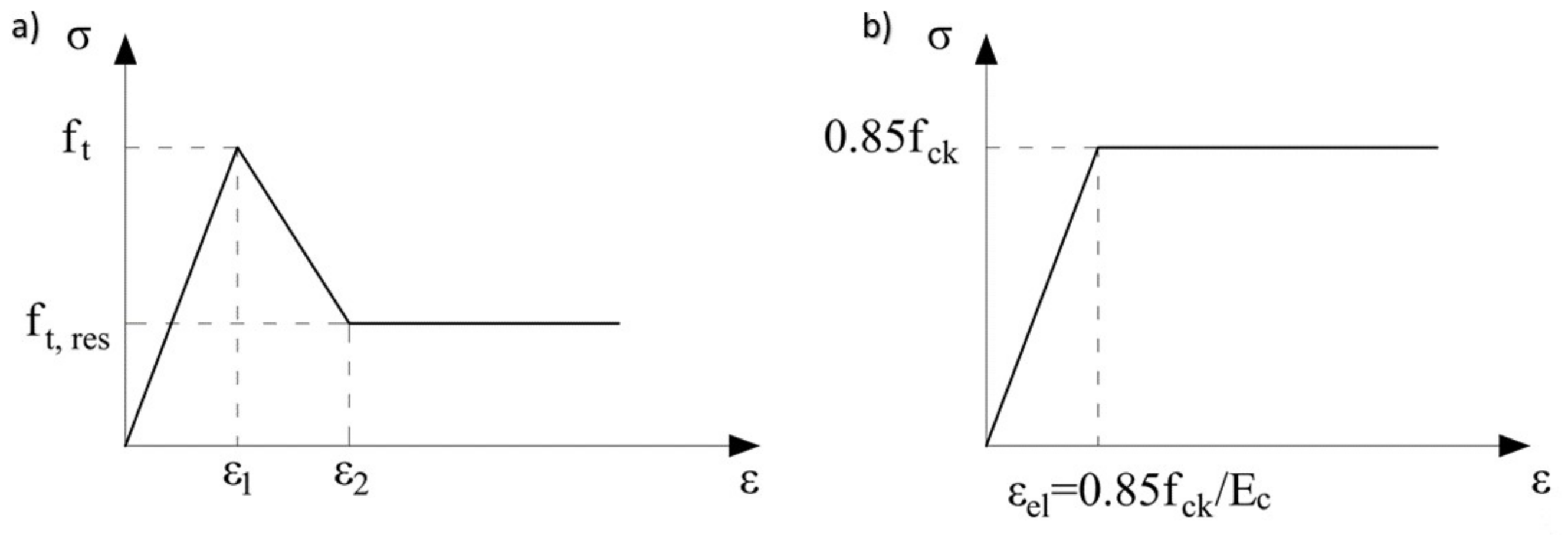
Figure 1.
Stress–strain relation in (a) tension and (b) compression.
3.1. Stress–Strain Relations
The effects of steel fibers on concrete mechanical behavior, such as the appearance of residual tensile strength, are accounted for by modifying the stress–strain relation of concrete (Figure 1). The stress–strain relations used in this study are based on those proposed by [27,28]. Compressive strength, elastic modulus, and the tensile strength of SFRC are assumed to have the same values as for plain concrete. Assuming that the compressive strength of the concrete is known, the equations defined for plain concrete are used to estimate the tensile strength (Equation (25) and the elastic modulus (Equation (28)) [28].
In compression, a bilinear stress–strain relation is used (Figure 1b). Peak compressive strength is estimated to be 85% of the characteristic compressive strength [29].
A trilinear stress–strain relation is used in tension (Figure 1a). Strain corresponding to the peak tensile strength, , can be calculated by dividing the peak tensile strength by the elastic modulus. Residual tensile strength is calculated using Equation (26), assuming that the tensile failure is due to fiber pullout, not fiber fracture. Coefficient a is used to account for the effect that different types of fibers have on the residual tensile strength. For example, due to their geometry, hooked fibers have a higher pullout strength than straight fibers, thus resulting in higher residual tensile strength. The values of the coefficient a are adopted as 1 for straight fibers, 1.5 for irregular fibers, and 2 for hook-end fibers, based on [27]. Strain (Equation (27)) (Figure 1a), after which residual tensile strength is assumed constant, is adopted from [11].
where:
- —volumetric fiber content
- —fiber factor format (i.e., aspect ratio)
- —characteristic compressive concrete strength
- —strain at peak tensile strength
- —residual tensile strength
- —tensile strength
- a—coefficient accounting for different types of fiber ( for straight fibers, for irregular fibers, for hooked fibers)
- —strain after which residual tensile strength is constant (Figure 1a)
Concrete stress–strain relations implemented in OpenSEES could not appropriately represent the proposed SFRC stress–strain relations. Therefore, the Elastic Multi-Linear model, whose nonlinear stress–strain relation is given by a multi-linear curve defined by a set of points, is used [25]. Steel in longitudinal bar reinforcement is modeled using the Giuffré–Menegotto–Pinto model (i.e., Steel02 in OpenSEES). The values of yield strength and elastic modulus varied among experiments and are given in [2,10,12]. The hardening ratio was assumed to be 0.01, and the parameters that control the transition from the elastic to the plastic branch of the steel stress–strain relation were , , for all specimens used for numerical model validation.
3.2. Probability Distribution of Model Parameters
Uncertainties in the material properties are quantified using probability distributions. Table 1 presents the probability distribution types and the assumed Coefficients of Variation (CoV). Mean values of the probability distributions of selected material properties can be obtained experimentally or using Equations (22)–(28). The probability distributions and their CoVs characterizing the uncertainties in concrete compressive and tensile strength, concrete elastic modulus, steel yield strength and steel elastic modulus are adopted based on the recommendations by Wisniweski et al. [30]. It is assumed that the CoVs of material properties defined for plain concrete can be used for SFRC, as the CoVs suggested by [30] are similar or lower to the CoVs of the SFRC’s material properties obtained experimentally [2,6].

Table 1.
Probability distribution of material properties.
Residual tensile strength of SFRC depends on the fiber orientation and the number of fibers crossing the crack, both of which are uncertain as they depend on the distribution of fibers along the specimen [31]. Borges et al. [5] and Tiberti et al. [6] experimentally investigated the post-cracking behavior of SFRC and quantified the uncertainties in the residual tensile strength for different crack openings, different displacement application rates, and casting directions. Based on these experimental results, a CoV of 35% is assumed for residual tensile strength. Similarly as for tensile strength, a lognormal distribution is assumed. The variance of geometric properties (e.g., concrete cover or rebar area), steel hardening ratio, fiber content and fiber aspect ratio are not considered in this study. Furthermore, the correlation between considered model inputs is not considered, as the Sobol’ method considers models with independent input variables.
3.3. Defining Characteristic Points of Beam Flexural Behavior
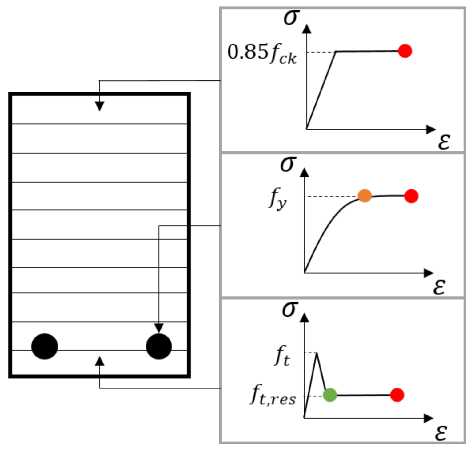
Three characteristic points in the flexural behavior of beams are identified in this study: the point when the first crack appears (i.e., the first-crack point); the point when longitudinal reinforcement starts to yield (i.e., the yield point) and the point when the beam collapses (i.e., the collapse point). Characteristic points are identified by following the stresses and strains in concrete and longitudinal reinforcement. Figure 2 illustrates how the characteristic points are defined. The appearance of the first crack in the beam is defined as the point when the concrete reaches its residual tensile strength. The yield point is defined as the point when the longitudinal reinforcement reaches its yield strength.
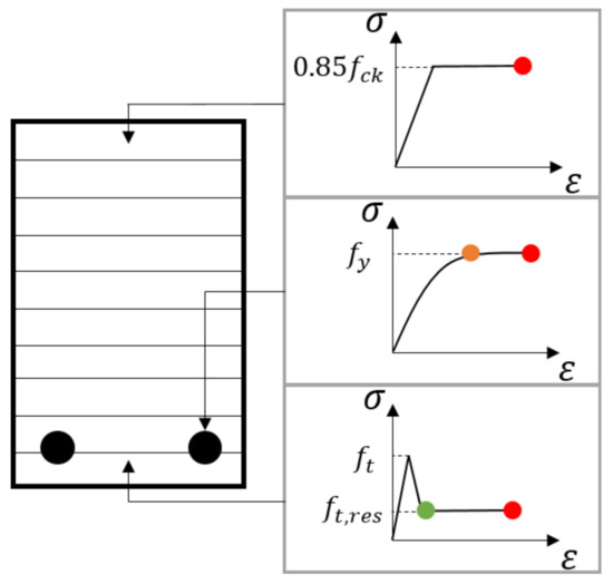
Figure 2.
Identifying characteristic points of beam bending using the stresses and strains in fiber cross-sections. The collapse point is represented in red, yield point in orange and first-crack point in green for the case of a beam cross-section exposed to pure bending. The bottom side is in tension, and the top side is compressed.
Different collapse definitions have been suggested in the literature. Some researchers define collapse by comparing the post-peak and peak loads (e.g., [32,33]). Such a definition is valid for structural elements that exhibit deflection-softening behavior. An alternative is to define maximal allowable strain values. This study uses one such criteria, as proposed by fib Model Code 2010 [34,35]. According to fib Model Code 2020 [34] bending failure (i.e., collapse) of an SFRC beam occurs when one of the following conditions is met:
- Attainment of the ultimate compressive strain in the SFRC;
- Attainment of the ultimate tensile strain in the longitudinal reinforcement;
- Attainment of the ultimate tensile strain in the SFRC.
The ultimate compressive strain for the adopted bilinear concrete stress–strain relation is between 2.4‰and 3.5‰, depending on the concrete compressive strength. The ultimate tensile strain in the longitudinal reinforcement is assumed to be 10% and the ultimate tensile strain in SFRC is equal to 2% for variable strain distribution along the cross-section [34]. Beam shear failure is not considered in this study.
4. Numerical Model Validation
The proposed numerical model is validated on four-point beam bending experiments available in the literature [2,10,12,36]. All experiments used for validation were performed on a beam reinforced with longitudinal reinforcement and steel fibers, loaded in thirds of the span with two vertical forces of equal intensity. The span-to-depth ratio of the beam was high enough to enable a dominant flexural behavior and all considered beam specimens failed in flexure. Beam parameters that varied among the specimens used for validation were the volumetric ratio of fibers (from 0.38% to 2%), fiber type (straight, irregular and hook-end), fiber aspect ratio (from 30 to 80), concrete strength (from 43 to 135 MPa), longitudinal reinforcement ratio (from 0.67% to 3.4%), beam span (from 1140 mm to 2100 mm) and cross-section dimensions. Details regarding specimens’ properties can be found in Table A1 in the Appendix A.
The flexural behavior of the beam is modeled using six finite elements of equal length with two integration points (i.e., cross-sections) per element (Figure 3). Each cross-section is discretized with 20 fibers along the height, representing SFRC and one fiber per bar of longitudinal reinforcement.
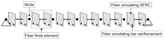
Figure 3.
Numerical model set-up.
Figure 4 compares the load-deflection relation obtained experimentally, using the proposed numerical model for specimen S2V1 tested by Oh [10]. The first crack, yield and collapse points are shown as green, orange and red circles, respectively, showing how the assumed criteria for defining these points compare to the experimentally obtained results. In this case, the numerical model was able to simulate the initial, post-crack, and post-yield stiffness of the beam and to capture the first crack, yield, and collapse points with good accuracy.
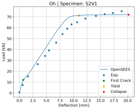
Figure 4.
Numerical model results for specimen S2V1 tested by Oh [10].
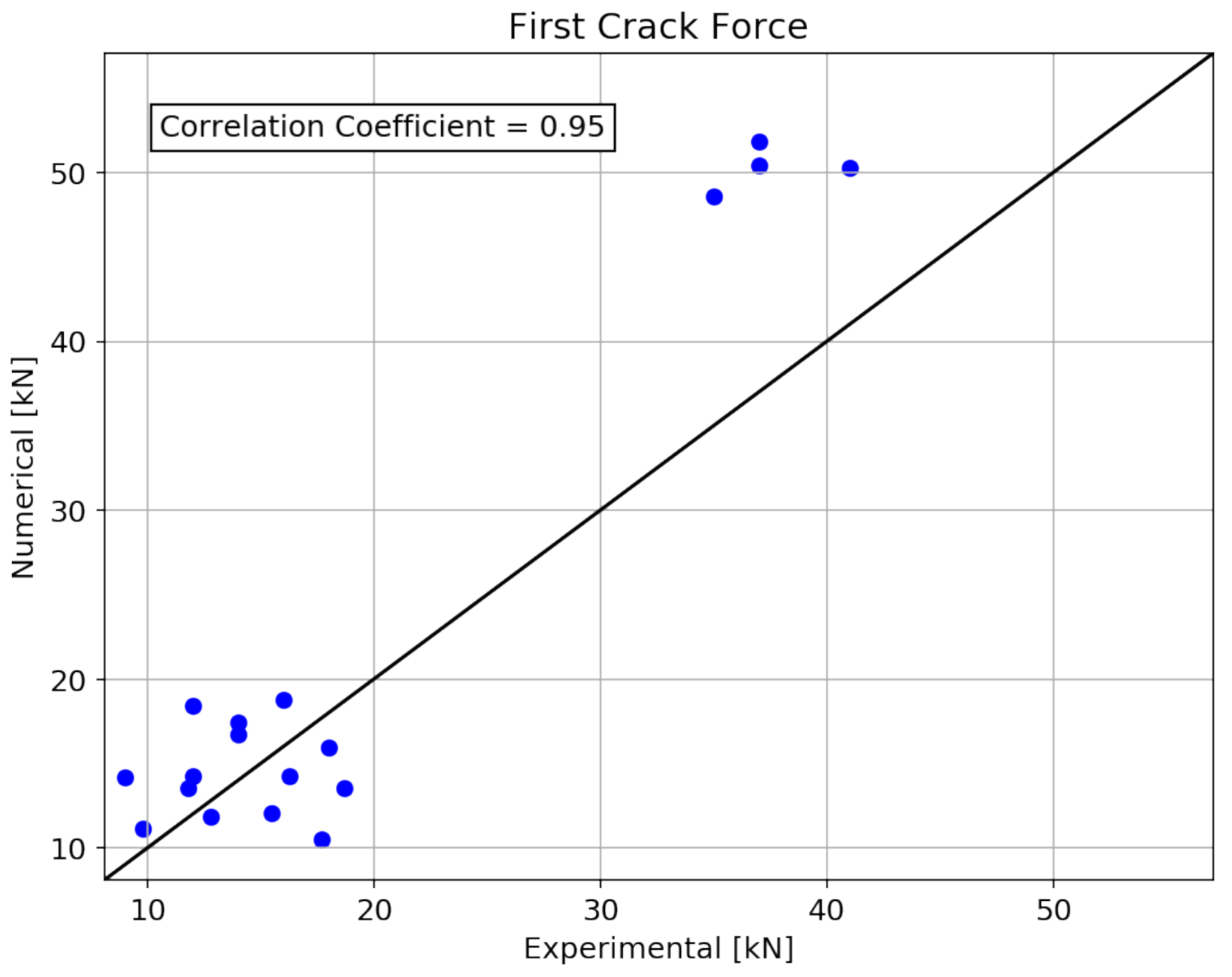
Figure 5 compares the experimentally and numerically obtained values of first-crack force for all specimens used for validation. The correlation coefficient between these values is relatively high, at 0.95. Figure 6 presents the relation between the experimentally and numerically obtained values of the first-crack displacement. The correlation coefficient between these values is lower than for the first-crack force, at 0.67. In the case of first-crack displacements, the numerical model almost always underestimated the experimentally obtained displacements. The reason for this underestimation might be that the numerical definition of the first crack point is too conservative since it is defined as the point at which only the bottom fiber of the numerical mid-span cross-section attains residual tensile strength. In the experimental setting, such crack might not have been noticed. For a more significant crack to form, perhaps the residual tensile strength should be attained in several fibers along the height of the cross-section in the numerical model. Nevertheless, the assumed first-crack definition remains on the safe side.
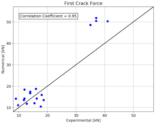
Figure 5.
Comparison between numerical and experimental results regarding first-crack force.
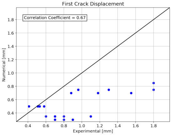
Figure 6.
Comparison between numerical and experimental results regarding first-crack displacement.
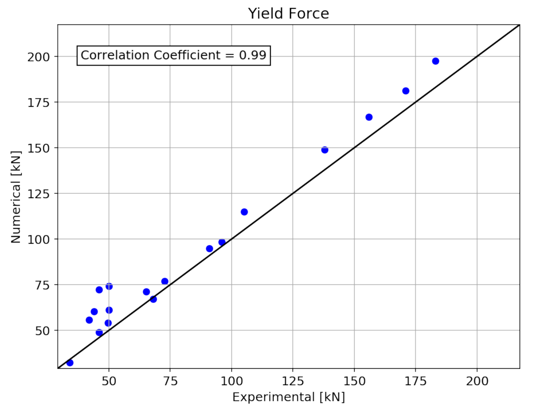
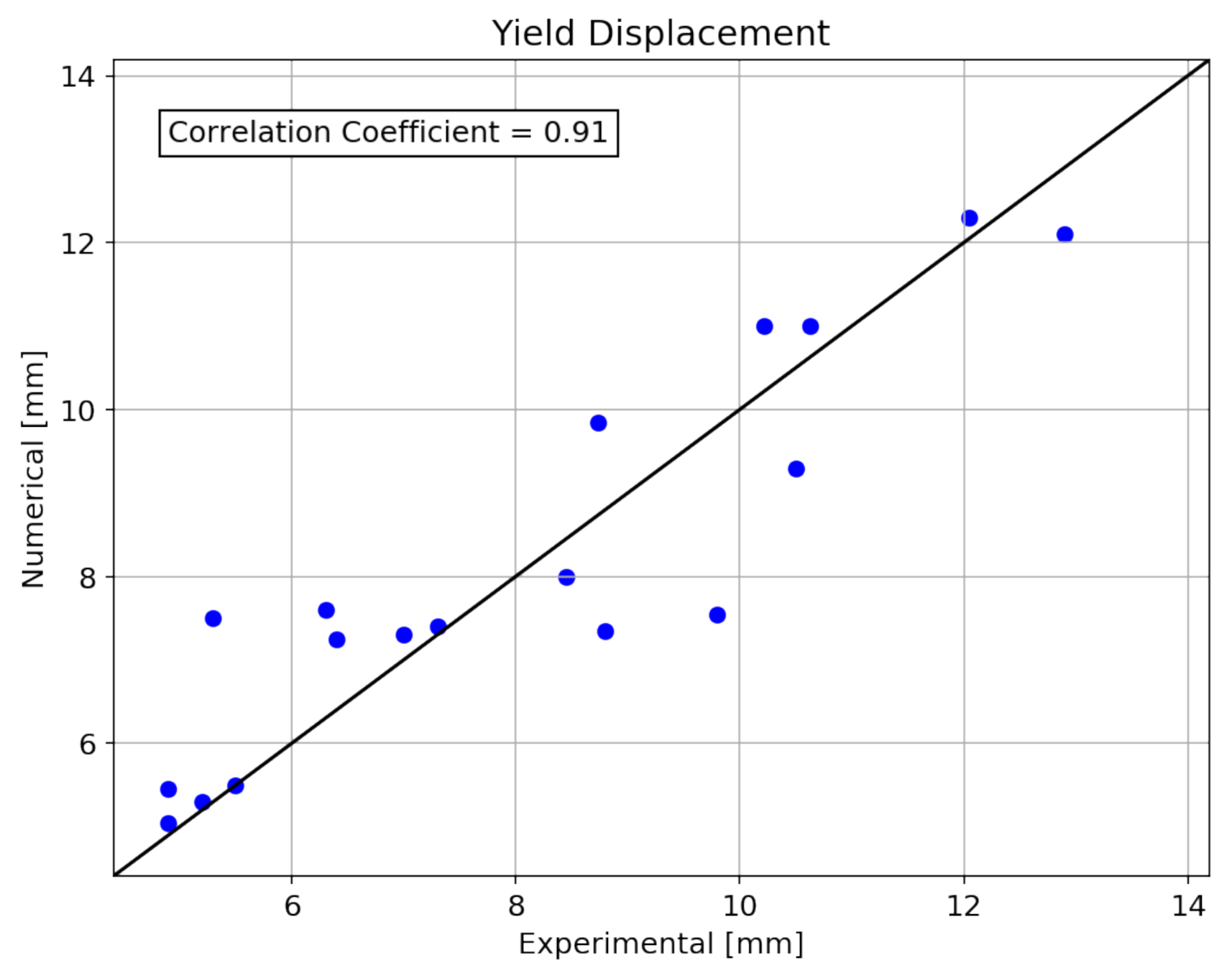
Figure 7 and Figure 8 show that the numerical model was able to predict the yield force and yield displacement with good accuracy, as the correlation coefficients between the numerical and experimental values are 0.99 and 0.91, respectively.
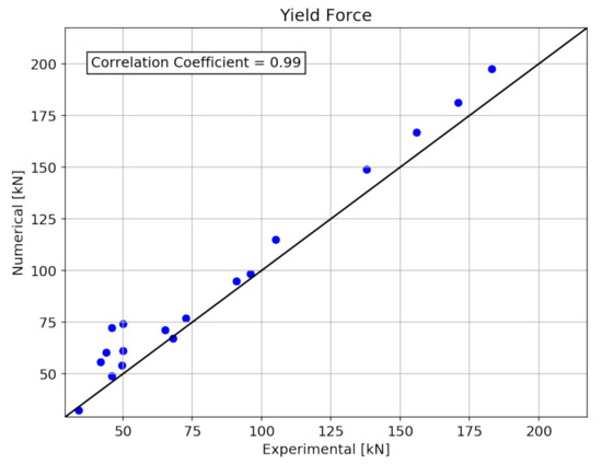
Figure 7.
Comparison between numerical and experimental results regarding yield force.
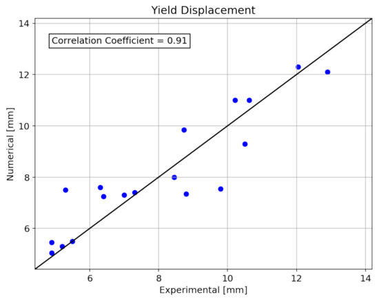
Figure 8.
Comparison between numerical and experimental results regarding yield displacement.
The correlation coefficient between collapse forces obtained numerically and experimentally is 0.99 (Figure 9). However, the ability of the numerical model to predict collapse displacement is significantly lower, as illustrated in Figure 10. One of the reasons might be that most of the experiments used for validation were load-controlled (red dots in Figure 10), thus the plateau in the load–deflection relation, where the displacement increases significantly, was not captured, underestimating the maximum displacement that the beam could attain. Therefore, load-controlled experiments might not be suitable for validating collapse displacements. Contrary, for all displacement-controlled experiments, the numerical model underestimated the collapse displacement, and thus remained on the safe side (Figure 10), which is most likely the goal of the collapse point criteria used in this paper and defined in fib Model Code 2010 [34].
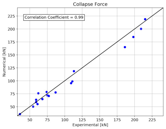
Figure 9.
Comparison between numerical and experimental results regarding collapse force.
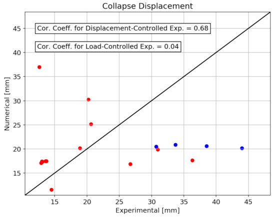
Figure 10.
Comparison between numerical and experimental results of displacement-controlled experiments regarding collapse displacement. Red dots mark load-controlled experiments. Blue dots mark displacement-controlled experiments.
Furthermore, the identification of the collapse point can be difficult in ductile elements where collapse is not as clearly defined as in brittle elements. The randomness in the structural behavior of SFRC also contributed to the large scatter of experimentally obtained collapse displacements, further reinforcing the need for probabilistic analysis and identification of the most important sources of this uncertainty. Nevertheless, the proposed FEM model can be improved to increase the accuracy of collapse prediction. Potential improvements would be to consider deflection-softening behavior of beams, by, for example, considering strain-softening in compression. Furthermore, other collapse definitions can be considered (e.g., [33]).
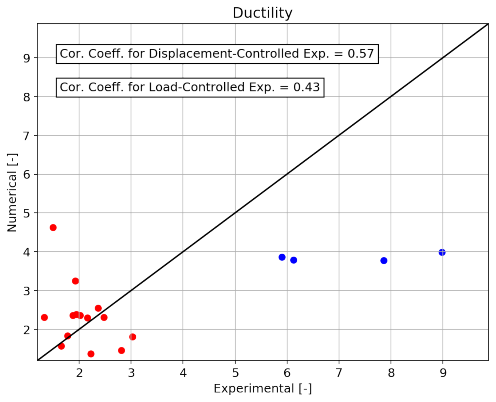
Ductility can be expressed by comparing curvatures [32], energies [37] or displacements [38] at ultimate (i.e., collapse) and yield states. In this study, ductility is defined as the ratio between the collapse and the yield displacement, a definition often used for SFRC beams [12,33,39]. Similarly as for collapse displacements, in the case of displacement-controlled experiments, the numerical model underestimated the ductility of the beams, remaining on the safe side (Figure 11). Due to the underestimation of beam’s collapse displacement in load-controlled experiments, numerical model’s estimates of beam ductility often overestimate experimentally obtained values.
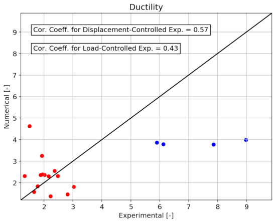
Figure 11.
Comparison between numerical and experimental results regarding the beam’s ductility factor. Red dots mark load-controlled experiments. Blue dots mark displacement-controlled experiments.
Table A2 in the Appendix A provides a summary of first-crack, yield, and collapse forces and displacements obtained experimentally and numerically for all specimens used for validation.
5. Case Study: SFRC Beam
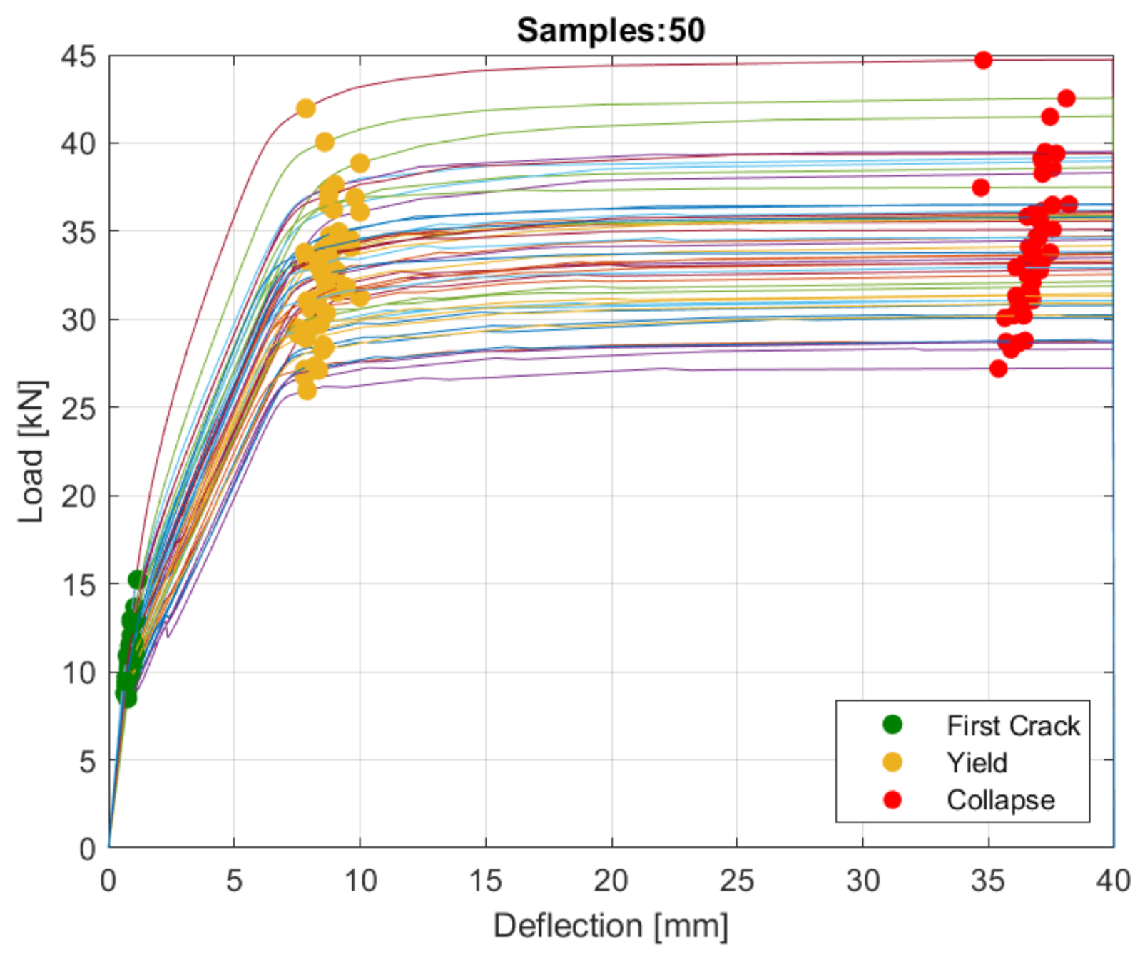
The RB-SF specimen tested by [2] is used as a case study to illustrate how the proposed numerical model and sensitivity analysis method can be used to identify material properties that are the main sources of uncertainty in the beam’s flexural behavior. To illustrate the probabilistic numerical model, 50 realizations of the proposed probabilistic numerical model are performed and the consequent load–deflection relations are presented in Figure 12. The probabilistic model of considered material properties is defined in UQLab software and linked with the numerical model defined in OpenSEESPy using UQLink [26,40,41]. The first-crack, yield, and collapse points are marked with green, orange, and red color, respectively. Higher variance of forces than displacements, related to the three characteristic points, can be observed from the presented results of the probabilistic numerical model, implying that the displacements are less sensitive to the variance of the considered material properties than forces.
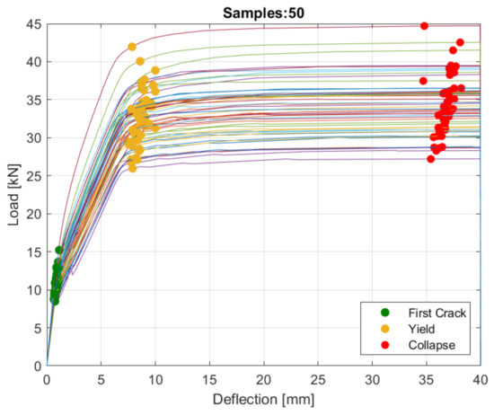
Figure 12.
Load–deflection relations for 50 realizations of the proposed probabilistic numerical model obtained using MC sampling.
5.1. PCE Metamodeling
The PCE metamodel of the probabilistic numerical model of the RB-SF specimen used in the previous section is obtained using the UQLab software [41]. Separate PCE metamodels are trained for each of the seven considered Quantities of Interest (QoIs): first-crack displacement and force; yield displacement and force, collapse displacement and force and ductility. An experimental design of 5000 samples is used to train PCEs for all QoIs. Adaptive PCE with a hyperbolic norm truncation scheme is used, and the accuracy of the PCE is measured using the leave-one-out error (LOO error). The details regarding the PCE metamodels for each of the considered QoIs are given in Table 2.
Table 2.
Degree, q-norm and LOO error of PCE metamodels.
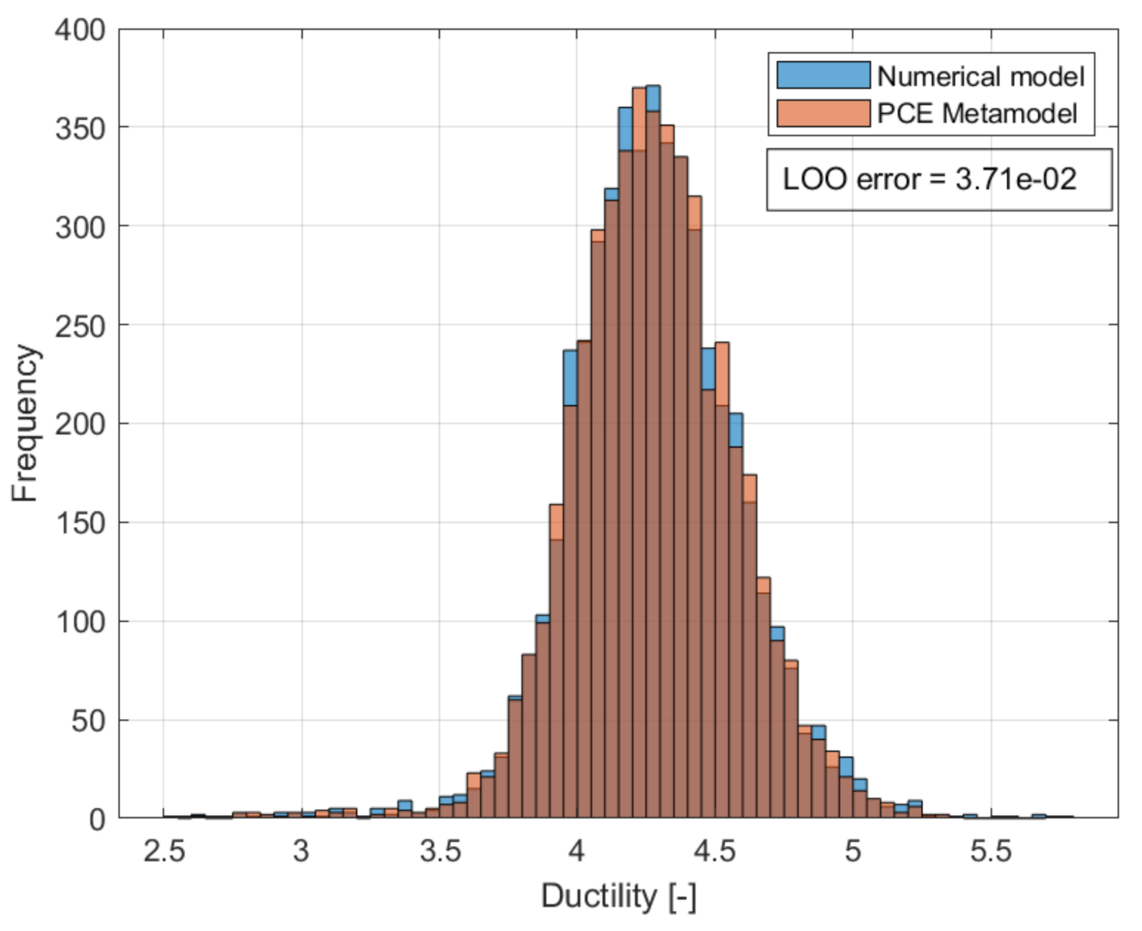
Figure 13 compares the histogram of the ductility values obtained from the probabilistic numerical model and from the corresponding PCE. A single run of the numerical model takes around 110 milliseconds, while the corresponding PCE metamodel takes 0.96 milliseconds on the same hardware, showing an acceleration of more than 100 times.

Figure 13.
Histogram of 500 samples of ductility factor values obtained using the numerical model and PCE metamodel.
5.2. Sensitivity Analysis
Figure 14, Figure 15, Figure 16, Figure 17, Figure 18, Figure 19and Figure 20 present the total Sobol’ indices for the forces and displacements of three characteristic points of the considered SFRC beams’ flexural behavior. Higher total Sobol’ index of a material property indicates that the variance of that material property has a higher effect on the variance of the considered QoI, and therefore, changing the value of that material property will have a larger effect on the considered QoI. Material properties with low total Sobol’ indices, can be set to a constant value (e.g., to their expected values) without significantly changing the variance of the considered QoI; therefore, the change in the values of material properties with low Sobol’ indices will not have a large effect on the considered QoI. This property can be used for dimensionality reduction [42].
Figure 14 and Figure 15 present total Sobol’ indices for first-crack force and displacement. The tensile strength of the SFRC has the highest total Sobol’ index of around 0.8. The variance of the residual tensile strength contributes around 20% to the variance of first-crack force and around 10% to the variance of the first-crack displacement. Furthermore, the variance of the elastic modulus of the SFRC is responsible for around 20% of variance of the first-crack displacement but has a very small effect on the first-crack force.
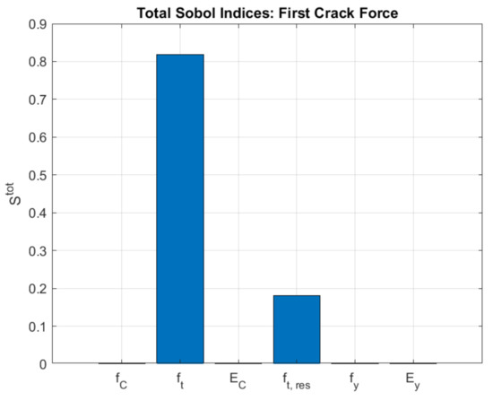
Figure 14.
Total Sobol’ indices for first-crack force.
Figure 14.
Total Sobol’ indices for first-crack force.

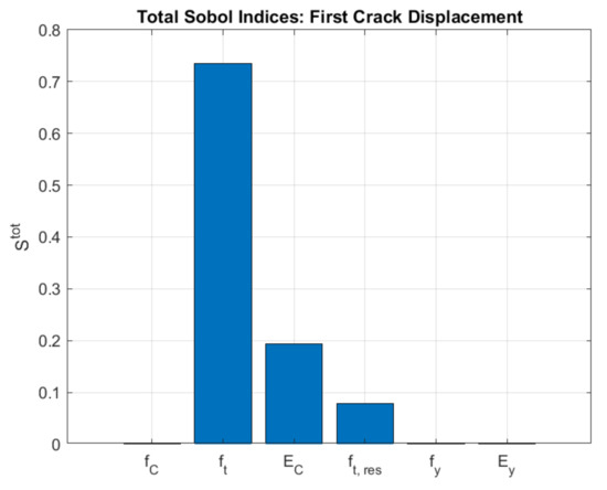
Figure 15.
Total Sobol’ indices for first-crack displacement.
Figure 15.
Total Sobol’ indices for first-crack displacement.

Figure 16 and Figure 17 present total Sobol’ indices for yield force and yield displacement. The variance of yield force is dominated by the variance of the SFRC’s residual tensile strength, accounting for around 90% of the variance. The variance of the yield strength of the bar reinforcement contributed only 10% to the variance of the yield force. However, despite the relatively low CoV of rebar yield strength of 5%, its variance contributed to 45% of the variance of yield displacement, indicating that rebar yield strength is very important for the yield displacement of the SFRC beam. The variance of residual tensile strength, SFRC’s elastic modulus, and tensile strength were also recognized as important sources of uncertainty in the case of the yield displacement.
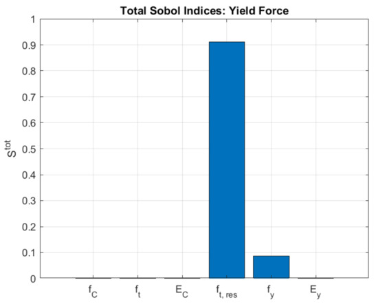
Figure 16.
Total Sobol’ indices for yield force.
Figure 16.
Total Sobol’ indices for yield force.

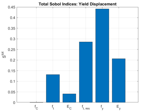
Figure 17.
Total Sobol’ indices for yield displacement.
Figure 17.
Total Sobol’ indices for yield displacement.

Total Sobol’ indices for collapse force and collapse displacement are presented in Figure 18 and Figure 19. Similarly as in the case of yield force, the variance of the collapse force was primarily caused by the variance of the SFRC’s residual tensile strength. The variance of the collapse displacement is also dominated by the variance of the SFRC’s residual tensile strength. The variance of the SFRC’s compressive strength was also important for the variance of the collapse displacement, probably due to certain cases in which beams achieved compression failure, as defined in Section 3.3.

Figure 18.
Total Sobol’ indices for collapse displacement.
Figure 18.
Total Sobol’ indices for collapse displacement.
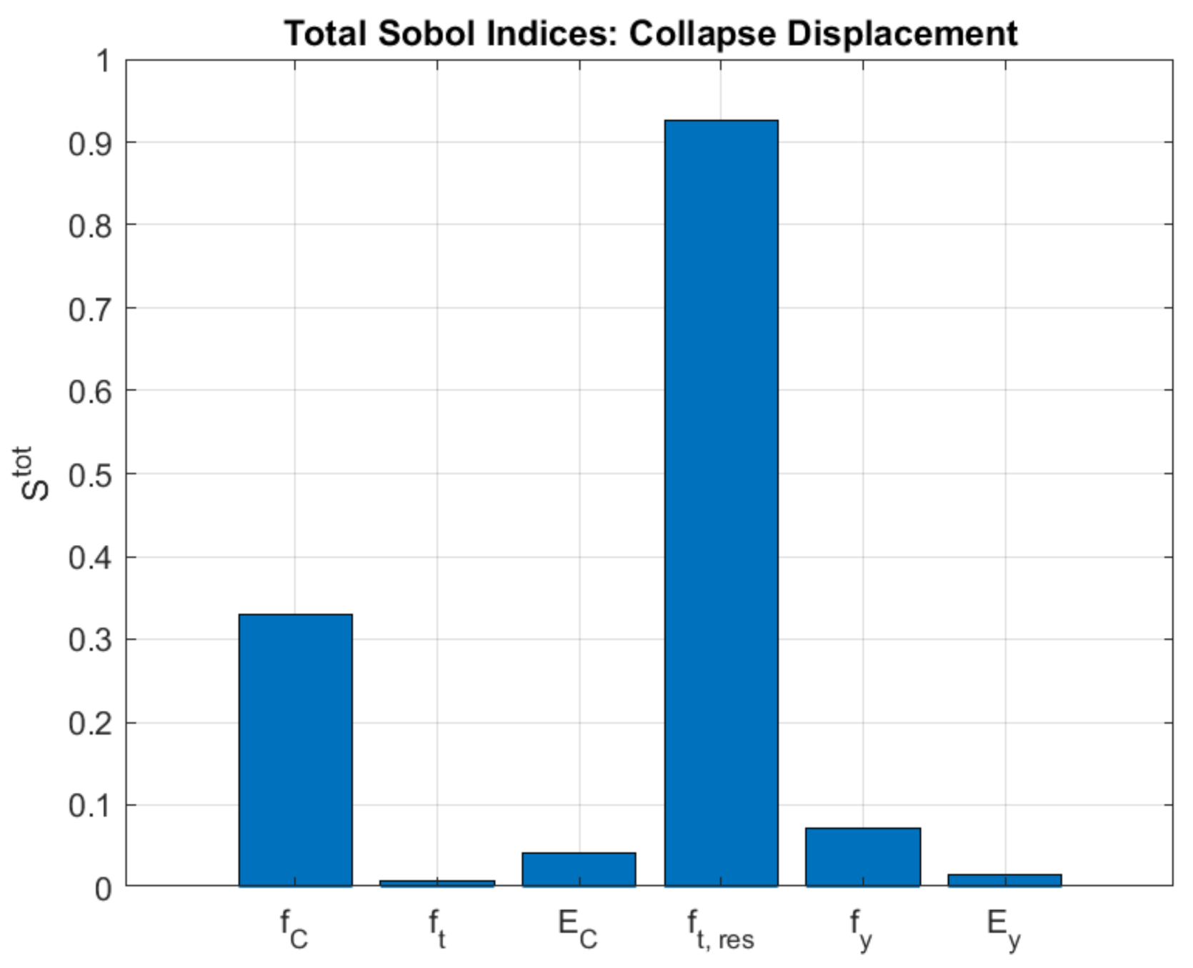

Figure 19.
Total Sobol’ indices for collapse force.
Figure 19.
Total Sobol’ indices for collapse force.

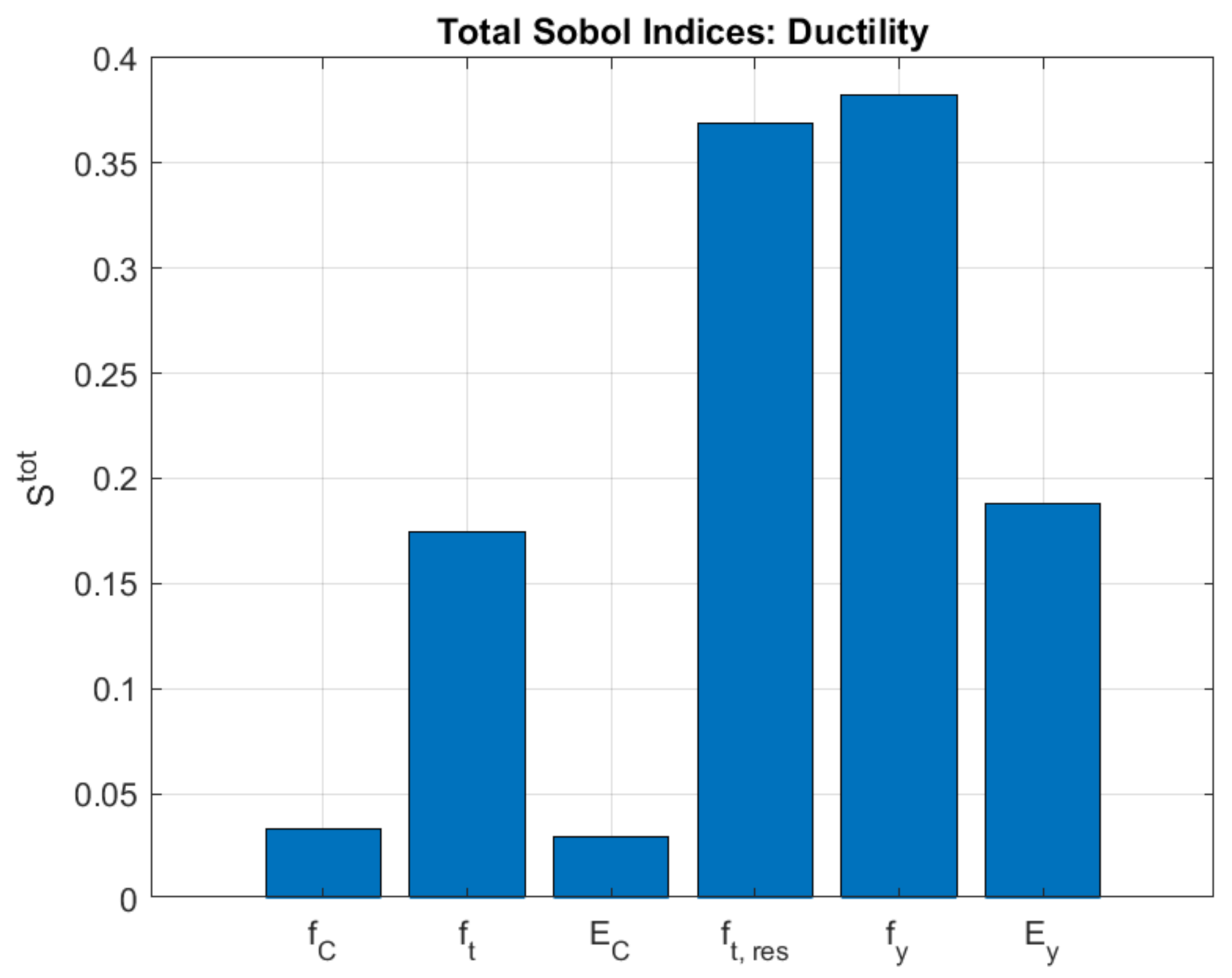
Figure 20 presents total Sobol’ indices for the ductility of the considered SFRC beam. As ductility is defined as the ratio between the collapse and yield displacement, the variance of the ductility depends on the variance of these two displacements. The variance of rebar yield strength and SFRC’s residual tensile strength contribute the most to the uncertainty in the SFRC beam’s ductility. This means that changing these two material properties is the most effective way to modify the beam’s ductility. Thus, the most effective way of increasing the ductility of the SFRC beam considered in this case study is by increasing the residual tensile strength of SFRC (e.g., by increasing the fiber dosage), thereby increasing the collapse displacement by delaying the attainment of 2% strain in tension. However, increasing the residual tensile strength after a certain point will not increase the beam’s collapse displacement, as other collapse conditions, such as attainment of maximal strain in compression might be achieved before reaching 2% strain in SFRC tension. Alternatively, the ductility can be increased by decreasing the rebar yield strength, decreasing the beam yield displacement and yield strength, without significantly affecting the beam’s collapse displacement (Figure 18).

Figure 20.
Total Sobol’ indices for ductility.
Figure 20.
Total Sobol’ indices for ductility.
6. Discussion and Conclusions
This paper combines global variance-based sensitivity analysis, (i.e., the Sobol’ method) with a fiber finite element model of SFRC beam’s flexural behavior to identify material properties whose uncertainty contributes the most to the uncertainty in the flexural behavior of an SFRC beam. To illustrate the proposed approach, a case study SFRC beam is presented. Results of the case study showed that the material parameter whose variance affected the variance of first-crack force and displacement the most (i.e., had the highest Sobol’ index) was concrete tensile strength. The variance of the yield point was mostly affected by the variance of residual tensile strength of concrete and yield strength and elastic modulus of the longitudinal reinforcement. Finally, residual tensile strength was the dominant source of uncertainty for the beam’s collapse point.
The results of the sensitivity analysis can be used to efficiently reduce the variance of SFRC beams’ flexural behavior, by reducing the variance of the material properties with high Sobol’ indices. For example, the variance of SFRC’s residual tensile strength, primarily caused by the random dispersion of fibers, can be reduced using casting procedures that lead to a more predictive distribution of fibers in the structural element (e.g., horizontal instead of vertical casting), by increasing the fiber content [6] or using advanced computational models to simulate the position and orientation of fibers in an SFRC element, reducing the uncertainty in the distribution of steel fibers along the structural element [43]. Furthermore, the results can help in understanding how changing the values of certain material properties will affect the flexural behavior of the SFRC beam. For example, in the presented case study it was identified that increasing the residual tensile strength will not significantly affect first-crack displacement and force, relevant for serviceability limit-states, but will affect the yield and collapse point.
It should be noted that the results of the Sobol’ analysis depend on the assumed probability distributions and their mean and variance values. Therefore, the results presented herein apply for the case of the assumed probability distributions for considered material properties (Table 1). Certain material properties might have low Sobol’ indices, due to the assumed low coefficient of variation, not due to their small relevance to the SFRC beam behavior. Furthermore, the limitations of the numerical model, such as its conservative estimation of collapse displacement, should be kept in mind.
Lastly, generalizing the conclusion obtained in this case study to beams of different geometric and material properties requires further analysis. Nevertheless, the presented methodology is applicable to beams of different dimensions and material properties, using the proposed numerical model or more advanced numerical models.
Author Contributions
Conceptualization, P.B. and N.B.; methodology, P.B. and N.B.; software, N.B.; validation, P.B. and N.B.; writing—original draft preparation, P.B., N.B. and D.K.; writing—review and editing, P.B., N.B. and D.K.; visualization, N.B.; supervision, P.B. and D.K.; funding acquisition, P.B. and D.K. All authors have read and agreed to the published version of the manuscript.
Funding
The publication of this research was supported by the company “Construction Center Ltd.” from Subotica, Serbia.
Acknowledgments
The second author appreciates insights provided by Professor Boris Jeremić from the University of California, Davis and Professor Božidar Stojadinović from the Chair of Structural Dynamics and Earthquake Engineering, ETH Zurich.
Conflicts of Interest
The authors declare no conflict of interest.
Appendix A
Table A1.
Properties of specimens used for numerical model validation.
Table A1.
Properties of specimens used for numerical model validation.
| Author | Specimen | B × H × L (mm) | (MPa) | Longitudinal Reinforcement Ratio (%) | (%) | Fiber Geometry | Fiber Factor Format |
|---|---|---|---|---|---|---|---|
| Blagojević et al. | RB-SF | 100 × 176 × 1920 | 69.17 | 0.67 | 1.5 | Irregular | 55 |
| Ning et al. | BS-A-SF30 | 200 × 300 × 2100 | 67 | 0.76 | 0.38 | Hooked | 80 |
| BS-A-SF50 | 0.64 | ||||||
| BS-B-SF30 | 0.96 | 0.38 | |||||
| BS-B-SF50 | 0.64 | ||||||
| Oh | S1V1 | 120 × 180 × 1800 | 43 | 1.5 | 1 | Straight | 57 |
| S1V2 | 47.8 | 2 | |||||
| S2V1 | 43 | 2.4 | 1 | ||||
| S2V2 | 47.8 | 2 | |||||
| D2V1 | 43 | 3.4 + 0.93 | 1 | ||||
| D2V2 | 47.8 | 2 | |||||
| Qi et al. | F1 | 120 × 140 × 1140 | 116 | 0.7 | 2 | Straight | 65 |
| F2 | 96.3 | 0.5 | |||||
| F3 | 94.3 | 1 | |||||
| F4 | 116 | 1.57 | 2 | ||||
| F6 | 120.5 | 0.7 | 30 | ||||
| F7 | 113.2 | 2 | |||||
| F9 | 135.6 | 65 |
Table A2.
Comparison of numerical and experimental results for three characteristic points used for numerical model validation.
Table A2.
Comparison of numerical and experimental results for three characteristic points used for numerical model validation.
| Author | Specimen | First Crack Point | Yield Point | Collapse Point | Ductility | ||||
|---|---|---|---|---|---|---|---|---|---|
| Force (kN) | Displ. (mm) | Force (kN) | Displ. (mm) | Force (kN) | Displ. (mm) | ||||
| Blagojević et al. | RB-SF | Exp. | 17.7 | 1.8 | 34 | 8.45 | 35.7 | 12.6 * | 1.5 |
| Num. | 10.52 | 0.85 | 32.32 | 8.0 | 35.89 | 37.00 | 4.62 | ||
| Ning et al. | BS-A-SF30 | Exp. | 35 | 0.53 | 138 | 4.9 | 186 | 44 | 8.98 |
| Num. | 48.59 | 0.5 | 149.03 | 5.05 | 165.14 | 20.15 | 4.00 | ||
| BS-A-SF50 | Exp. | 37 | 0.58 | 156 | 5.2 | 198 | 30.7 | 5.9 | |
| Num. | 50.45 | 0.5 | 167.02 | 5.3 | 184.67 | 20.5 | 3.87 | ||
| BS-B-SF30 | Exp. | 41 | 0.51 | 171 | 4.9 | 209 | 38.5 | 7.86 | |
| Num. | 50.27 | 0.5 | 181.23 | 5.45 | 200.28 | 20.6 | 3.78 | ||
| BS-B-SF50 | Exp. | 37 | 0.41 | 183 | 5.5 | 215 | 33.7 | 6.13 | |
| Num. | 51.87 | 0.5 | 197.67 | 5.5 | 219.01 | 20.85 | 3.79 | ||
| Oh | S1V1 | Exp. | 9.8 | 0.88 | 45.9 | 10.5 | 54.76 | 20.2 * | 1.92 |
| Num. | 11.16 | 0.7 | 49.05 | 9.3 | 50.22 | 30.25 | 3.25 | ||
| S1V2 | Exp. | 12.8 | 1.18 | 49.55 | 8.73 | 60.98 | 20.63 * | 2.36 | |
| Num. | 11.86 | 0.7 | 54.12 | 9.85 | 55.14 | 25.15 | 2.55 | ||
| S2V1 | Exp. | 15.5 | 1.55 | 65.15 | 10.63 | 75 | 18.9 * | 1.78 | |
| Num. | 12.06 | 0.7 | 71.27 | 11.0 | 71.95 | 20.15 | 1.83 | ||
| S2V2 | Exp. | 18.67 | 1.8 | 72.6 | 10.22 | 86.7 | 30.94 * | 3.03 | |
| Num. | 13.53 | 0.75 | 76.89 | 11.0 | 77.71 | 19.9 | 1.81 | ||
| D2V1 | Exp. | 11.8 | 0.96 | 91 | 12.9 | 109 | 36.3 * | 2.81 | |
| Num. | 13.58 | 0.75 | 94.75 | 12.1 | 95.44 | 17.65 | 1.46 | ||
| D2V2 | Exp. | 16.27 | 1.3 | 96 | 12.05 | 110.74 | 26.72 * | 2.22 | |
| Num. | 14.28 | 0.75 | 98.42 | 12.3 | 99.13 | 16.85 | 1.37 | ||
| Qi et al. | F-1 | Exp. | 14 | 0.7 | 46 | 6.3 | 62 | 13.6 * | 2.16 |
| Num. | 17.44 | 0.35 | 72.35 | 7.6 | 75.97 | 17.5 | 2.3 | ||
| F-2 | Exp. | 9 | 0.7 | 42 | 7.0 | 59 | 13.6 * | 1.94 | |
| Num. | 14.19 | 0.3 | 55.77 | 7.3 | 58.89 | 17.45 | 2.39 | ||
| F-3 | Exp. | 12 | 0.8 | 44 | 7.3 | 59 | 13.7 * | 1.88 | |
| Num. | 14.23 | 0.3 | 60.44 | 7.4 | 63.48 | 17.5 | 2.36 | ||
| F-4 | Exp. | 12 | 0.6 | 105 | 8.8 | 113 | 14.5 * | 1.65 | |
| Num. | 18.44 | 0.35 | 115.12 | 7.35 | 118.54 | 11.55 | 1.57 | ||
| F-6 | Exp. | 18 | 0.9 | 50 | 6.4 | 68 | 12.9 * | 2.02 | |
| Num. | 15.96 | 0.3 | 61.16 | 7.25 | 64.79 | 17.1 | 2.36 | ||
| F-6 | Exp. | 18 | 0.9 | 50 | 6.4 | 68 | 12.9 * | 2.02 | |
| Num. | 15.96 | 0.3 | 61.16 | 7.25 | 64.79 | 17.1 | 2.36 | ||
| F-7 | Exp. | 14 | 0.8 | 68 | 9.8 | 77 | 13.0 * | 1.33 | |
| Num. | 16.73 | 0.35 | 67.27 | 7.55 | 70.8 | 17.4 | 2.3 | ||
| F-9 | Exp. | 16 | 1.1 | 50 | 5.3 | 74 | 13.1 * | 2.47 | |
| Num. | 18.78 | 0.35 | 74.27 | 7.5 | 78.5 | 17.35 | 2.31 | ||
* marks load-controlled experiments.
References
- Aviram, A.; Stojadinović, B.; Parra-Montesinos, G.J. High-performance fiber-reinforced concrete bridge columns under bidirectional cyclic loading. ACI Struct. J 2014, 111, 303–312. [Google Scholar] [CrossRef]
- Blagojević, P.; Blagojević, N.; Kukaras, D.; Živković, D.; Šutanovac, D. Mechanical Flexural Properties of Concrete with Melt-extract Stainless Steel Fibres. Gradjevinar 2020, 72, 1155–1164. [Google Scholar] [CrossRef]
- Purkiss, J.A.; Blagojević, P. Comparison between the short and long term behaviour of fibre reinforced and unreinforced concrete beams. Compos. Struct. 1993, 25, 45–49. [Google Scholar] [CrossRef]
- Hasgul, U.; Yavas, A.; Birol, T.; Turker, K. Steel Fiber Use as Shear Reinforcement on I-Shaped UHP-FRC Beams. Appl. Sci. 2019, 9, 5526. [Google Scholar] [CrossRef] [Green Version]
- Borges, L.A.C.; Monte, R.; Rambo, D.A.S.; de Figueiredo, A.D. Evaluation of post-cracking behavior of fiber reinforced concrete using indirect tension test. Constr. Build. Mater. 2019, 204, 510–519. [Google Scholar] [CrossRef]
- Tiberti, G.; Germano, F.; Mudadu, A.; Plizzari, G.A. An overview of the flexural post-cracking behavior of steel fiber reinforced concrete. Struct. Concr. 2018, 19, 695–718. [Google Scholar] [CrossRef]
- Cunha, V.M.; Barros, J.A.; Sena-Cruz, J.M. A finite element model with discrete embedded elements for fibre reinforced composites. Comput. Struct. 2012, 94–95, 22–33. [Google Scholar] [CrossRef] [Green Version]
- Bitencourt, A.G.; Manzoli, O.L.; Bittencourt, T.N.; Vecchio, F.J. Numerical modeling of steel fiber reinforced concrete with a discrete and explicit representation of steel fibers. Int. J. Solids. Struct. 2019, 159, 171–190. [Google Scholar] [CrossRef]
- Purkiss, J.A.; Wilson, P.J.; Blagojević, P. Determination of the load-carrying capacity of steel fibre reinforced cocnrete beams. Compos. Struct 1997, 38, 111–117. [Google Scholar] [CrossRef]
- Oh, B.H. Flexural Analysis of Reinforced Concrete Beams Containing Steel Fibers. J. Struct. Eng. 1993, 118, 2821–2835. [Google Scholar] [CrossRef]
- Barros, J.A.; Cunha, V.M.; Ribeiro, A.F.; Antunes, J.A. Post-cracking behaviour of steel fibre reinforced concrete. Mater. Struct. 2005, 38, 47–56. [Google Scholar] [CrossRef]
- Qi, J.; Wang, J.; Ma, Z.J. Flexural response of high-strength steel-ultra-high-performance fiber reinforced concrete beams based on a mesoscale constitutive model: Experiment and theory. Struct. Concr. 2018, 19, 719–734. [Google Scholar] [CrossRef]
- Buzzini, D.; Dazio, A.; Trüb, M. Quasi-Static Cyclic Tests on Three Hybrid Fibre Concrete Structural Walls; Technical Report; ETH Zürich: Zürich, Switzerland, 2006. [Google Scholar]
- Zhan, Y.; Meschke, G. Multilevel Computational Model for Failure Analysis of Steel-Fiber–Reinforced Concrete Structures. J. Eng. Mech. 2016, 142, 04016090. [Google Scholar] [CrossRef]
- JCSS. Probabilistic Model Code; Technical Report; Joint Committee on Structural Safety: Zurich, Switzerland, 2000; ISBN 978-3-909386-79-6. [Google Scholar]
- Sobol’, I.M. Sensitivity Estimates for Nonlinear Mathematical Models. Math. Comput. Model. 1993, 1, 407–414. [Google Scholar]
- Sobol’, I.M. Global sensitivity indices for nonlinear mathematical models and their Monte Carlo estimates. Math. Comput. Simul. 2001, 55, 271–280. [Google Scholar] [CrossRef]
- Homma, T.; Saltelli, A. Importance measures in global sensitivity analysis of model output. Reliab. Eng. Syst. Saf. 1996, 52, 1–17. [Google Scholar] [CrossRef]
- Saltelli, A. Making best use of model evaluations to compute sensitivity indices. Comput. Phys. Commun. 2002, 145, 280–297. [Google Scholar] [CrossRef]
- Sudret, B. Global sensitivity analysis using polynomial chaos expansion. Reliab. Eng. Syst. Saf. 2008, 93, 964–979. [Google Scholar] [CrossRef]
- Marelli, S.; Lüthen, N.; Sudret, B. UQLab User Manual—Polynomial Chaos Expansions; Chair of Risk, Safety and Uncertainty Quantification, ETH Zurich: Zurich, Switzerland, 2021. [Google Scholar]
- Blatman, G. Adaptive Sparse Polynomial Chaos Expansions for Uncertainty Propagation and Sensitivity Analysis. Ph.D. Thesis, Blaise Pascal University, Aubière, France, 2009. [Google Scholar]
- Berveiller, M.; Sudret, B.; Lemaire, M. Stochastic finite element: A non intrusive approach by regression. Eur. J. Comput. Mech. 2006, 15, 81–92. [Google Scholar] [CrossRef] [Green Version]
- Kaba, S.A.; Mahin, S.A. Refined Modelling of Reinforced Concrete Columns for Seismic Analysis; Report No. UCB/EERC-84/03; University of California: Berkeley, CA, USA, 1984. [Google Scholar]
- McKenna, F.; Fenves, G.L.; Scott, M.H.; Jeremić, B. Open System for Earthquake Engineering Simulation (OpenSees). 2000. Available online: http://opensees.berkeley.edu (accessed on 30 September 2021).
- Zhu, M.; McKenna, F.; Scott, M.H. OpenSeesPy: Python library for the OpenSees finite element framework. SoftwareX 2018. [Google Scholar] [CrossRef]
- Singh, H. Flexural Modeling of Steel Fiber-Reinforced Concrete Members: Analytical Investigations. Pract. Period. Struct. Des. Constr. 2015, 20, 04014046. [Google Scholar] [CrossRef]
- Soranakom, C.; Mobasher, B. Flexural design of fiber-reinforced concrete. ACI Mater. J. 2009, 106, 461–469. [Google Scholar] [CrossRef]
- Lok, T.S.; Xiao, J.R. Flexural Strength Assessment of Steel Fiber Reinforced Concrete. J. Mater. Civ. Eng. 1999, 11, 188–196. [Google Scholar] [CrossRef]
- Wiśniewski, D.F.; Cruz, P.J.; Henriques, A.A.R.; Simões, R.A. Probabilistic models for mechanical properties of concrete, reinforcing steel and pre-stressing steel. Struct. Infrastruct. Eng. 2012, 8, 111–123. [Google Scholar] [CrossRef]
- Lee, S.C.; Oh, J.H.; Cho, J.Y. Fiber orientation factor on rectangular cross-section in concrete members. Int. J. Eng. Technol. Innov. 2015, 7, 470–473. [Google Scholar] [CrossRef] [Green Version]
- Renić, T.; Kišiček, T. Ductility of Concrete Beams Reinforced with FRP Rebars. Buildings 2021, 11, 424. [Google Scholar] [CrossRef]
- Xu, S.; Wu, C.; Liu, Z.; Han, K.; Su, Y.; Zhao, J.; Li, J. Experimental investigation of seismic behavior of ultra-high performance steel fiber reinforced concrete columns. Eng. Struct. 2017, 152, 129–148. [Google Scholar] [CrossRef]
- CEB-FIP. fib Model Code for Concrete Structures 2010; Wilhelm Ernst & Sohn: Berlin, Germany, 2013. [Google Scholar]
- Trindade, Y.T.; Bitencourt, L.A.; Manzoli, O.L. Design of SFRC members aided by a multiscale model: Part II – Predicting the behavior of RC-SFRC beams. Compos. Struct. 2020, 241, 112079. [Google Scholar] [CrossRef]
- Ning, X.; Ding, Y.; Zhang, F.; Zhang, Y. Experimental study and prediction model for flexural behavior of reinforced SCC beam containing steel fibers. Constr. Build. Mater. 2015, 93, 644–653. [Google Scholar] [CrossRef] [Green Version]
- Sun, Z.Y.; Yang, Y.; Qin, W.H.; Ren, S.T.; Wu, G. Experimental study on flexural behavior of concrete beams reinforced by steel-fiber reinforced polymer composite bars. J. Reinf. Plast. Compos. 2012, 31, 1737–1745. [Google Scholar] [CrossRef]
- Paulay, T.; Priestley, M.J.N. Seismic Design of Reinforced Concrete and Masonry Buildings; John Wiley and Sons: Hoboken, NJ, USA, 1992. [Google Scholar]
- Sahoo, D.R.; Sharma, A. Effect of steel fiber content on behavior of concrete beams with and without stirrups. ACI Struct. J. 2014, 111, 1157–1166. [Google Scholar] [CrossRef]
- Moustapha, M.; Marelli, S.; Sudret, B. UQLab User Manual—The UQLink Module; Chair of Risk, Safety and Uncertainty Quantification, ETH Zurich: Zurich, Switzerland, 2021. [Google Scholar]
- Marelli, S.; Sudret, B. UQLab: A Framework for Uncertainty Quantification in MATLAB. In Proceedings of the 2nd International Conference on Vulnerability and Risk Analysis and Management (ICVRAM 2014), Liverpool, UK, 13–16 July 2014; pp. 2554–2563. [Google Scholar] [CrossRef] [Green Version]
- Abbiati, G.; Broccardo, M.; Abdallah, I.; Marelli, S.; Paolacci, F. Seismic fragility analysis based on artificial ground motions and surrogate modeling of validated structural simulators. Earthq. Eng. Struct. Dyn. 2021, 50, 2314–2333. [Google Scholar] [CrossRef]
- Gudžulić, V.; Dang, T.S.; Meschke, G. Computational modeling of fiber flow during casting of fresh concrete. Comput. Mech. 2019, 63, 1111–1129. [Google Scholar] [CrossRef]


Publisher’s Note: MDPI stays neutral with regard to jurisdictional claims in published maps and institutional affiliations. |
© 2021 by the authors. Licensee MDPI, Basel, Switzerland. This article is an open access article distributed under the terms and conditions of the Creative Commons Attribution (CC BY) license (https://creativecommons.org/licenses/by/4.0/).