
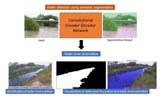
Deep Learning Semantic Segmentation for Water Level Estimation Using Surveillance Camera

 , ,
, ,
Abstract
:
1. Introduction
2. Methodology
2.1. Data Collection and Preparation
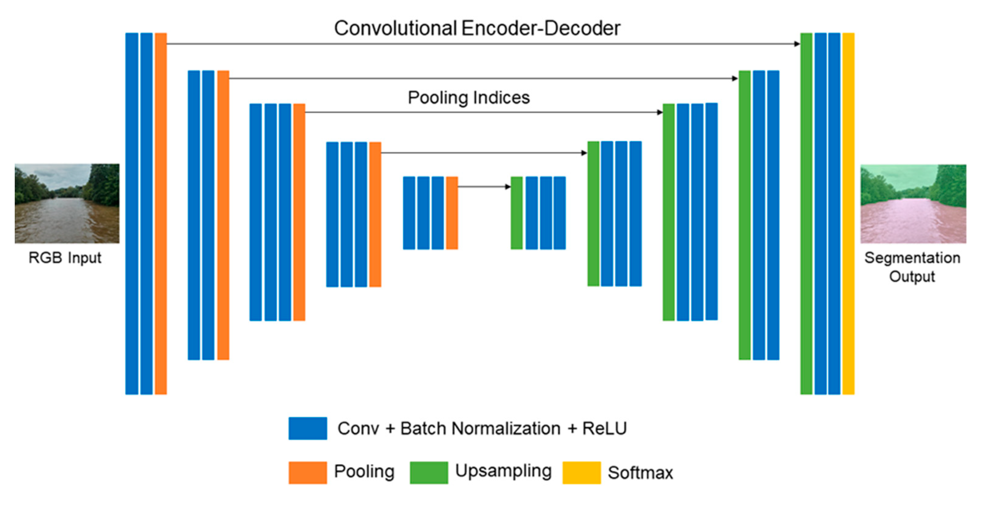
2.2. Semantic Segmentation Architecture
2.2.1. DeeplabV3+
2.2.2. SegNet
2.2.3. Hyperparameters Configuration
2.2.4. Data Augmentation
2.3. Segmentation Workflow: DeeplabV3+ Versus SegNet
2.3.1. Training Phase
2.3.2. Inference Phase
2.4. Segmentation Evaluation Metrics
2.5. Water Level Observation
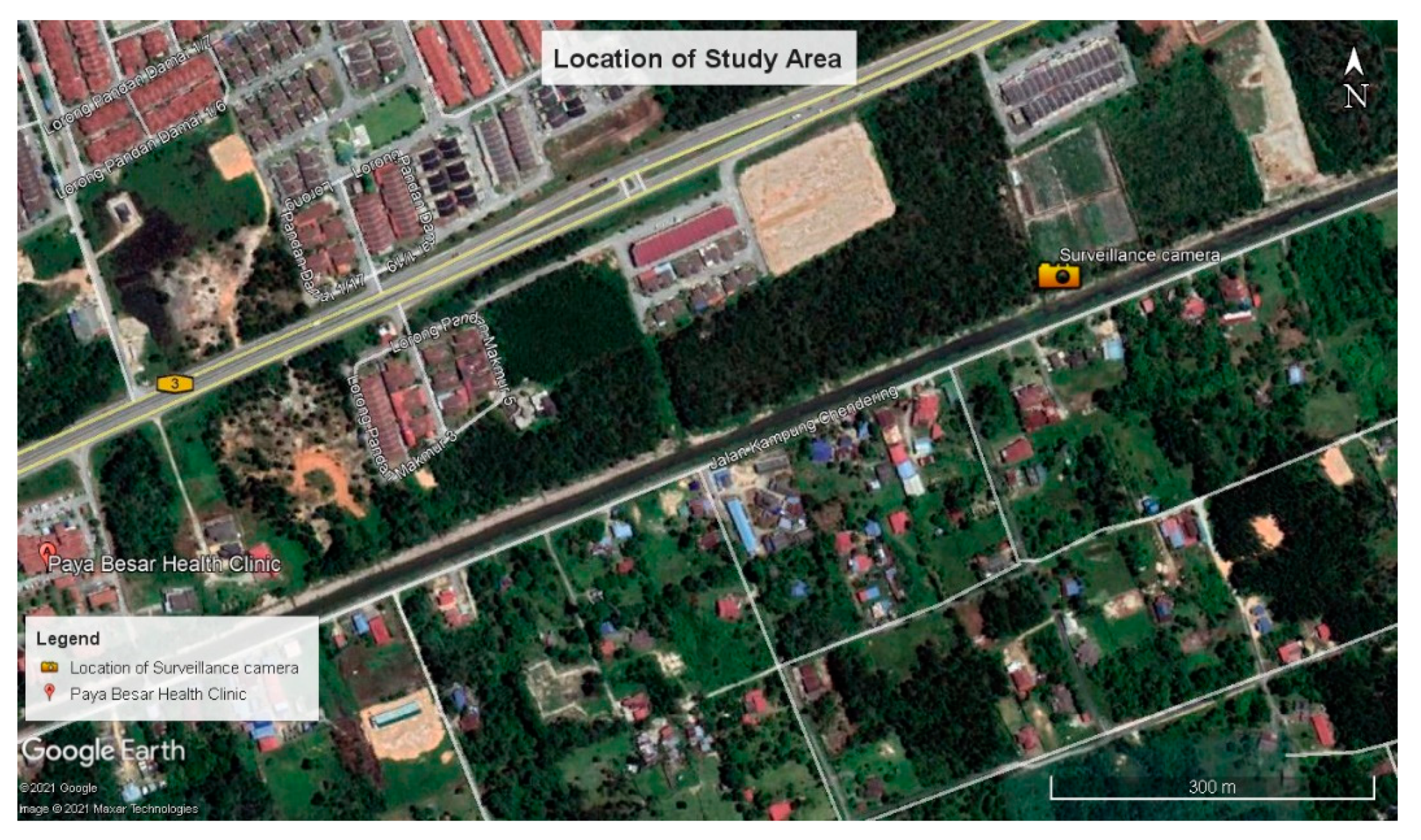
2.5.1. Study Area
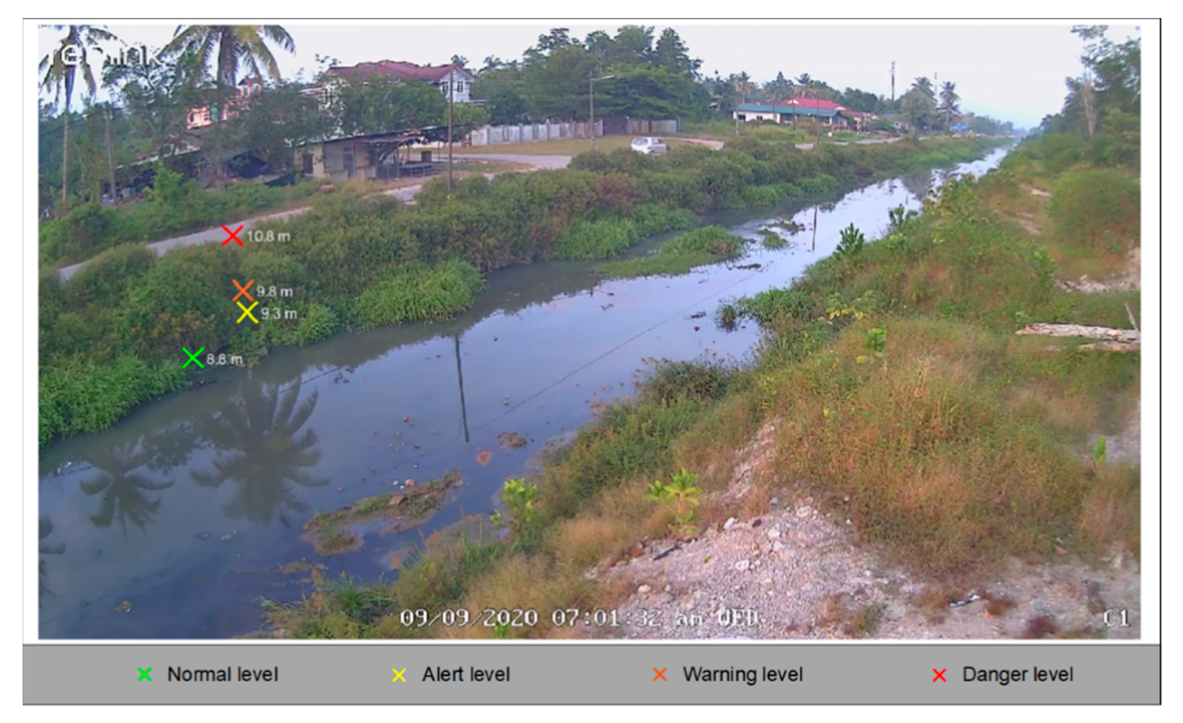
2.5.2. Water Level Framework
3. Results
3.1. Water Segmentation
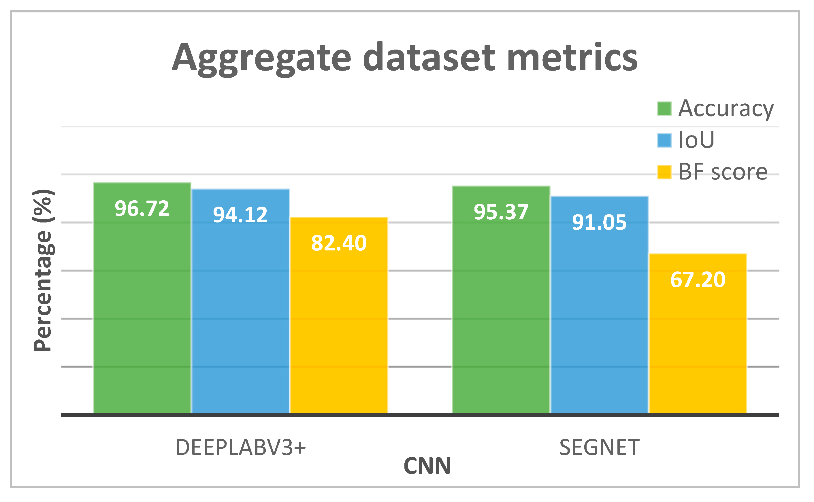
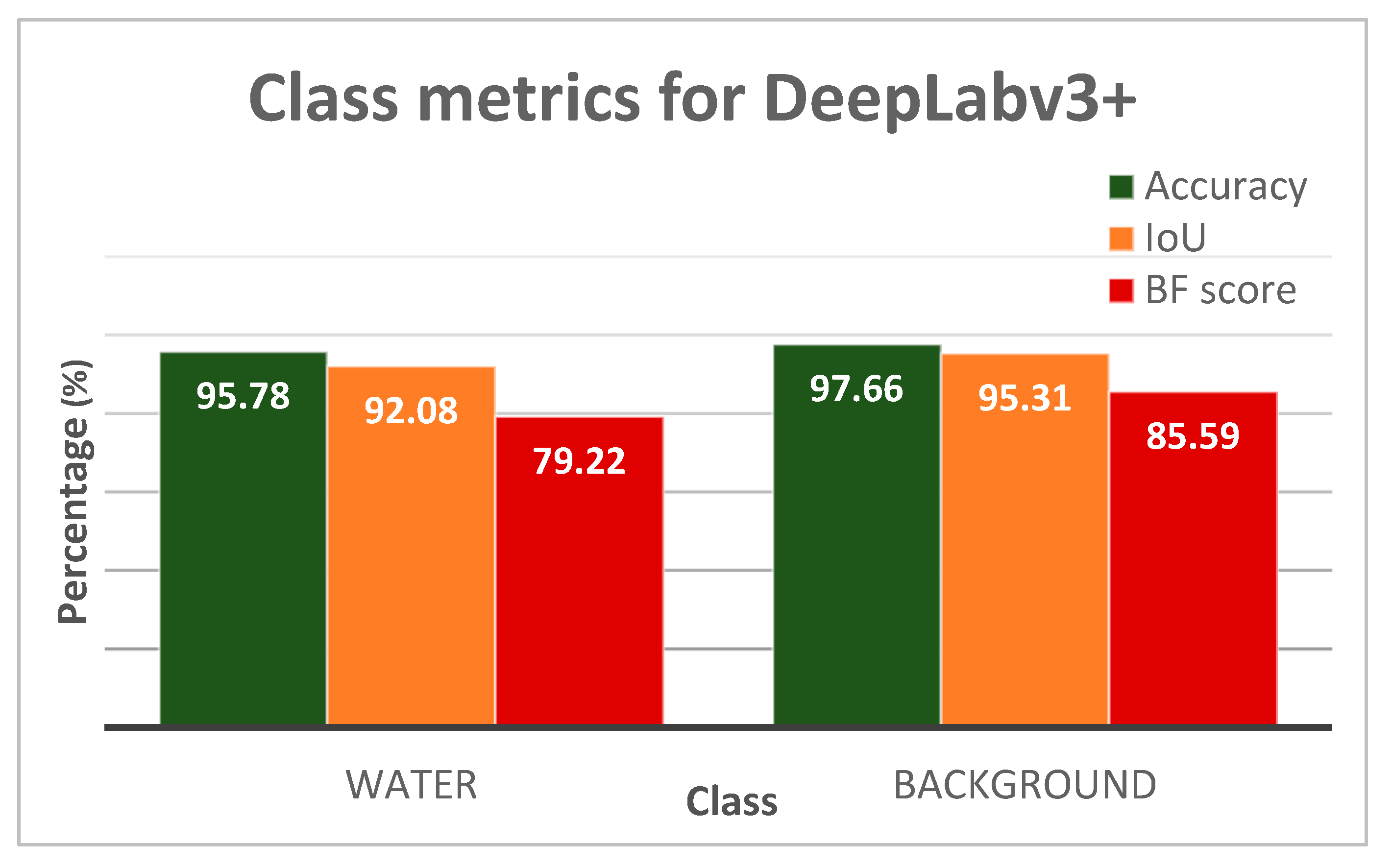
3.1.1. Performance Evaluation
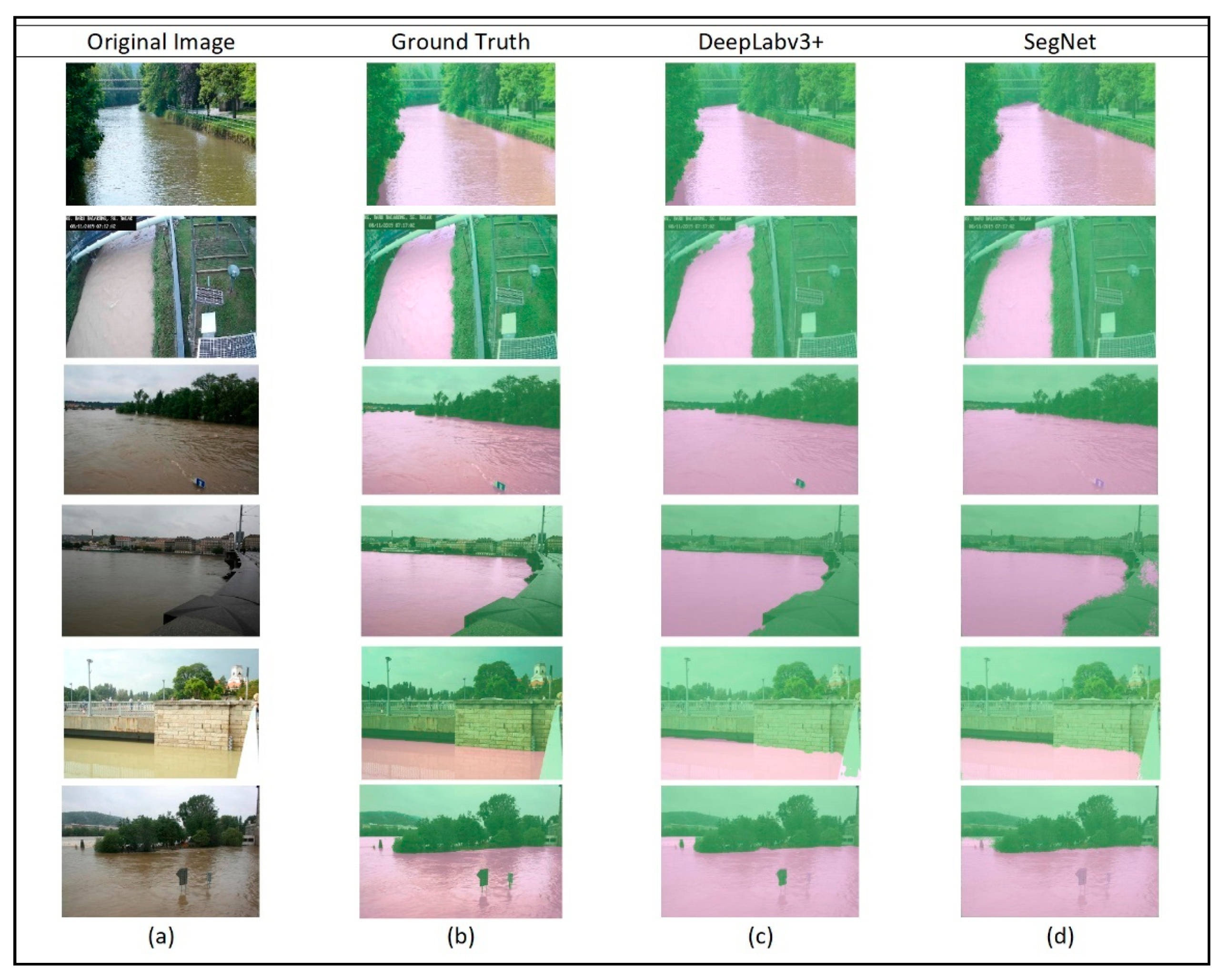
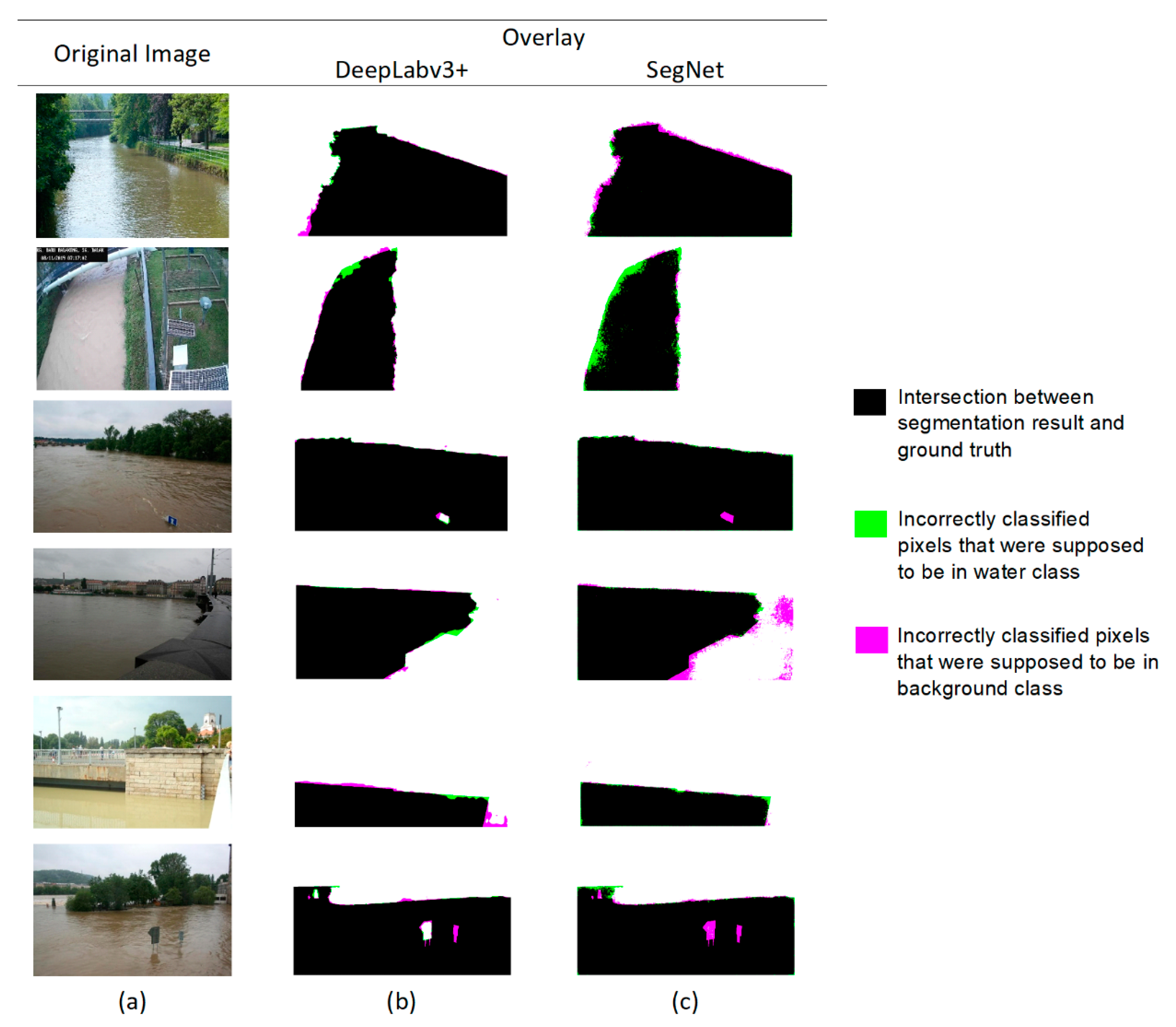
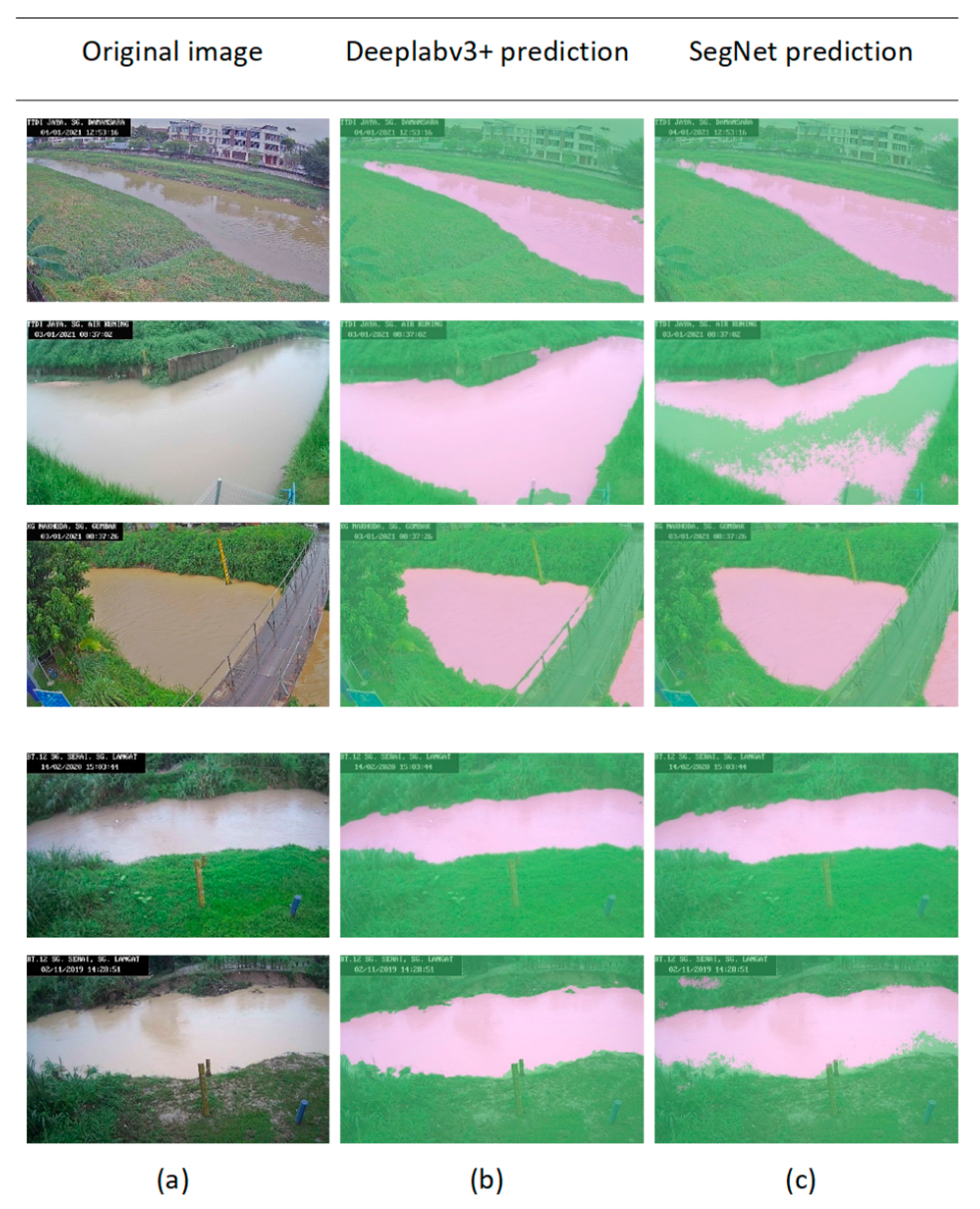
3.1.2. Visual Analysis of the Segmentation Results
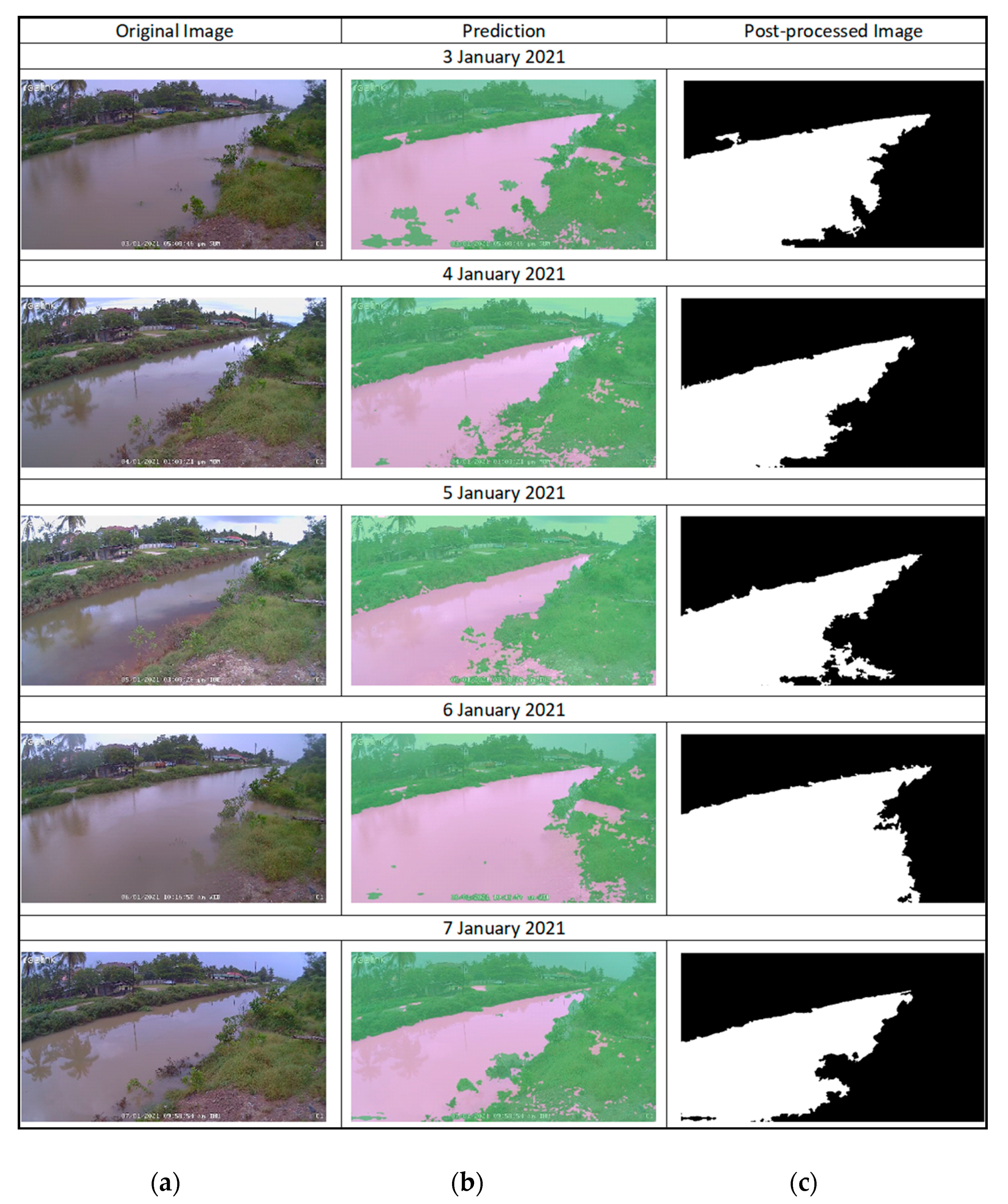
3.2. Inference Phase
3.3. Comparison with Previous Findings
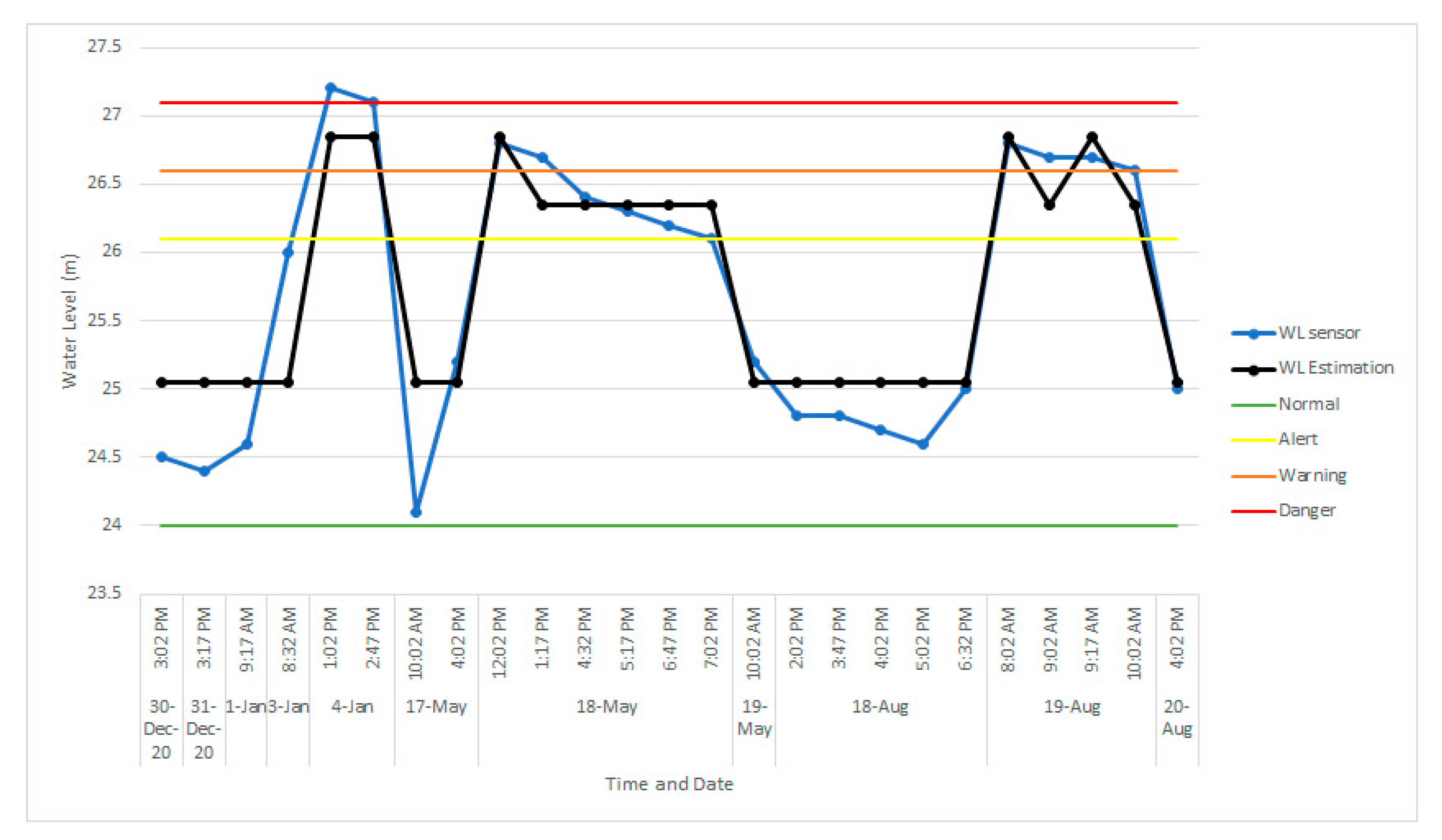
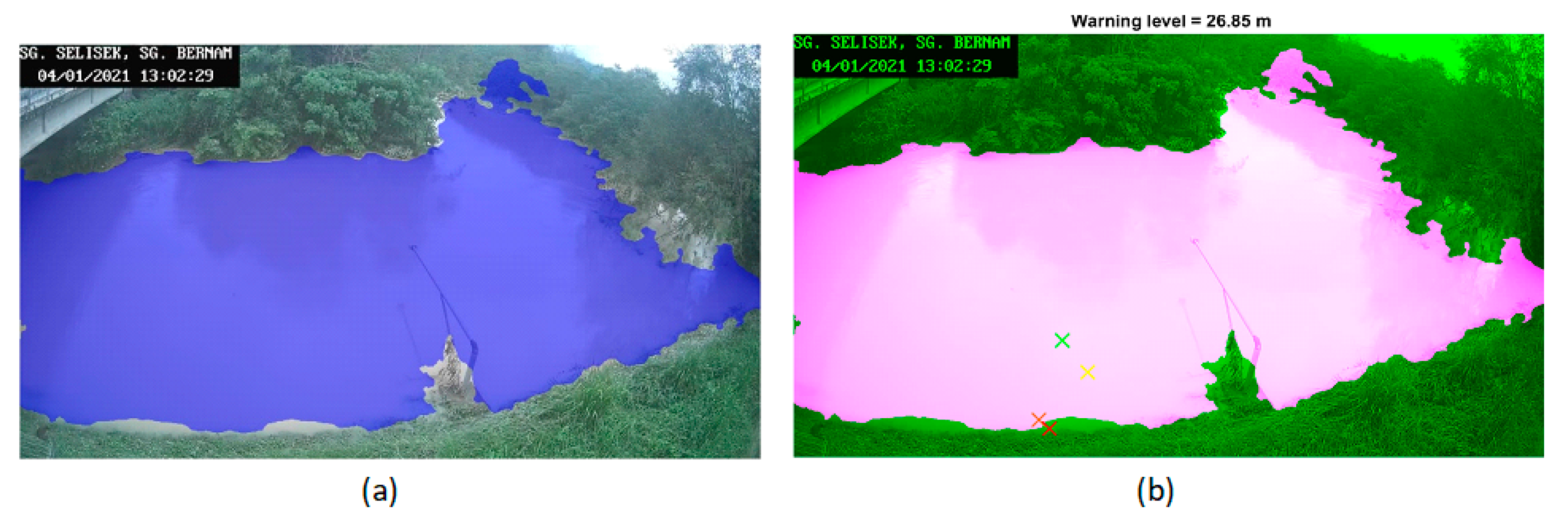
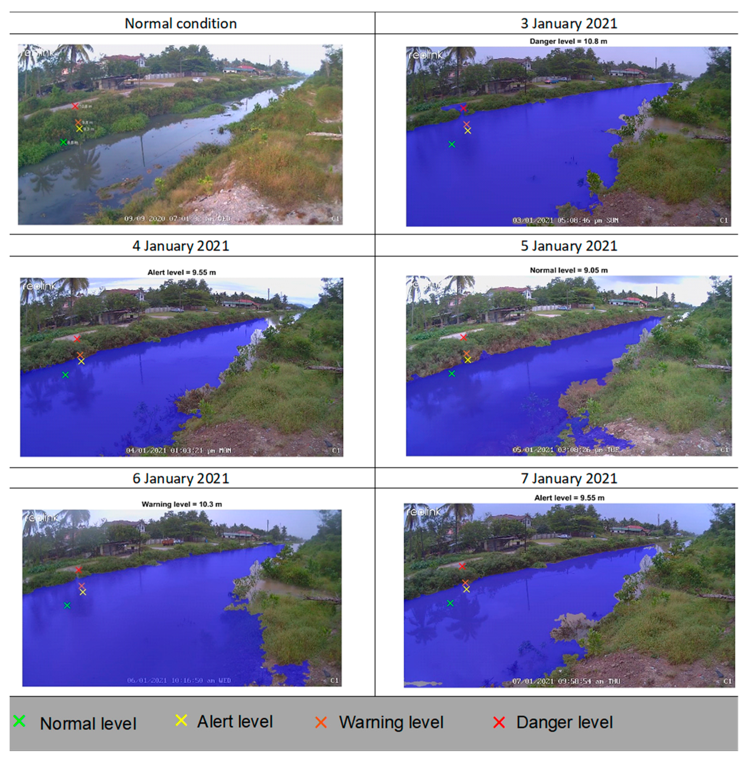
3.4. Practical Application for Water Level Observation
4. Discussion
5. Conclusions
Author Contributions
Funding
Institutional Review Board Statement
Informed Consent Statement
Data Availability Statement
Acknowledgments
Conflicts of Interest
References
- Demski, C.; Capstick, S.; Pidgeon, N.; Sposato, R.G.; Spence, A. Experience of extreme weather affects climate change mitigation and adaptation responses. Clim. Chang. 2017, 140, 149–164. [Google Scholar] [CrossRef] [Green Version]
- Wan Ruslan Ismail, T.H. Extreme weather and floods in Kelantan state, Malaysia in December 2014. Res. Mar. Sci. 2018, 3, 231–244. [Google Scholar]
- Azimi, M.A.; Syed Zakaria, S.A.; Majid, T.A. Disaster risks from economic perspective: Malaysian scenario. IOP Conf. Ser. Earth Environ. Sci. 2019, 244, 012009. [Google Scholar] [CrossRef]
- Blunden, J.; Boyer, T. State of the Climate in 2020. Bull. Amer. Meteor. Soc. 2021, 102, 1–475. [Google Scholar] [CrossRef]
- UNDRR. The Human Cost of Disasters—An Overview of the Last 20 Years 2000–2019; UNDRR: Geneva, Switzerland, 2020. [Google Scholar]
- Matgen, P.; Schumann, G.; Henry, J.B.; Hoffmann, L.; Pfister, L. Integration of SAR-derived river inundation areas, high-precision topographic data and a river flow model toward near real-time flood management. Int. J. Appl. Earth Obs. Geoinf. 2007, 9, 247–263. [Google Scholar] [CrossRef]
- Mason, D.C.; Davenport, I.J.; Neal, J.C.; Schumann, G.J.P.; Bates, P.D. Near real-time flood detection in urban and rural areas using high-resolution synthetic aperture radar images. IEEE Trans. Geosci. Remote Sens. 2012, 50, 3041–3052. [Google Scholar] [CrossRef] [Green Version]
- Skakun, S.; Kussul, N.; Shelestov, A.; Kussul, O. Flood Hazard and Flood Risk Assessment Using a Time Series of Satellite Images: A Case Study in Namibia. Risk Anal. 2014, 34, 1521–1537. [Google Scholar] [CrossRef] [PubMed]
- García-pintado, J.; Mason, D.C.; Dance, S.L.; Cloke, H.L.; Neal, J.C.; Freer, J.; Bates, P.D. Satellite-supported flood forecasting in river networks: A real case study. J. Hydrol. 2015, 523, 706–724. [Google Scholar] [CrossRef] [Green Version]
- Huang, X.; Wang, C.; Li, Z. GIS A near real-time flood-mapping approach by integrating social media and post-event satellite imagery. Ann. GIS 2018, 24, 113–123. [Google Scholar] [CrossRef]
- DID. DID Manual (Volume 1—Flood Management); Jabatan Pengairan dan Saliran Malaysia: Kuala Lumpur, Malaysia, 2009; Volume 1. [Google Scholar]
- Marin-Perez, R.; García-Pintado, J.; Gómez, A.S. A real-time measurement system for long-life flood monitoring and warning applications. Sensors 2012, 12, 4213–4236. [Google Scholar] [CrossRef] [PubMed]
- Ji, Y.; Zhang, M.; Wang, Y.; Wang, P.; Wang, A.; Wu, Y.; Xu, H.; Zhang, Y. Microwave-Photonic Sensor for Remote Water-Level Monitoring Based on Chaotic Laser. Int. J. Bifurc. Chaos 2014, 24, 1450032. [Google Scholar] [CrossRef]
- Lo, S.W.; Wu, J.H.; Lin, F.P.; Hsu, C.H. Cyber surveillance for flood disasters. Sensors 2015, 15, 2369–2387. [Google Scholar] [CrossRef] [PubMed] [Green Version]
- Kang, W.; Xiang, Y.; Wang, F.; Wan, L.; You, H. Flood detection in gaofen-3 SAR images via fully convolutional networks. Sensors 2018, 18, 2915. [Google Scholar] [CrossRef] [Green Version]
- Yang, C.; Wei, Y.; Wang, S.; Zhang, Z.; Huang, S. Extracting the flood extent from satellite SAR image with the support of topographic data. In Proceedings of the 2001 International Conferences on Info-Tech and Info-Net: A Key to Better Life, ICII 2001—Proceedings, Beijing, China, 29 October–1 November 2001; Volume 1, pp. 87–92. [Google Scholar]
- Cao, H.; Zhang, H.; Wang, C.; Zhang, B. Operational flood detection using Sentinel-1 SAR data over large areas. Water 2019, 11, 786. [Google Scholar] [CrossRef] [Green Version]
- Jung, H.C.; Jasinski, M.; Kim, J.W.; Shum, C.K.; Bates, P.; Neal, J.; Lee, H.; Alsdorf, D. Calibration of two-dimensional floodplain modeling in the central Atchafalaya Basin Floodway System using SAR interferometry. Water Resour. Res. 2012, 48, 1–13. [Google Scholar] [CrossRef] [Green Version]
- Schumann, G.J.P.; Neal, J.C.; Mason, D.C.; Bates, P.D. The accuracy of sequential aerial photography and SAR data for observing urban flood dynamics, a case study of the UK summer 2007 floods. Remote Sens. Environ. 2011, 115, 2536–2546. [Google Scholar] [CrossRef]
- Feng, Q.; Liu, J.; Gong, J. Urban flood mapping based on unmanned aerial vehicle remote sensing and random forest classifier-A case of yuyao, China. Water 2015, 7, 1437–1455. [Google Scholar] [CrossRef]
- Perks, M.T.; Russell, A.J.; Large, A.R.G. Technical note: Advances in flash flood monitoring using unmanned aerial vehicles (UAVs). Hydrol. Earth Syst. Sci. 2016, 20, 4005–4015. [Google Scholar] [CrossRef] [Green Version]
- Langhammer, J.; Bernsteinová, J.; Miřijovský, J. Building a high-precision 2D hydrodynamic flood model using UAV photogrammetry and sensor network monitoring. Water 2017, 9, 861. [Google Scholar] [CrossRef]
- Lindner, G.; Schraml, K.; Mansberger, R.; Hübl, J. UAV monitoring and documentation of a large landslide. Appl. Geomatics 2016, 8, 1–11. [Google Scholar] [CrossRef]
- Nishar, A.; Richards, S.; Breen, D.; Robertson, J.; Breen, B. Thermal infrared imaging of geothermal environments and by an unmanned aerial vehicle (UAV): A case study of the Wairakei—Tauhara geothermal field, Taupo, New Zealand. Renew. Energy 2016, 86, 1256–1264. [Google Scholar] [CrossRef]
- Wierzbicki, D.; Kedzierski, M.; Fryskowska, A. Assesment of the influence of UAV image quality on the orthophoto production. Int. Arch. Photogramm. Remote Sens. Spat. Inf. Sci. 2015, 40, 1–8. [Google Scholar] [CrossRef] [Green Version]
- Muhadi, N.A.; Abdullah, A.F.; Bejo, S.K.; Mahadi, M.R.; Mijic, A. The Use of LiDAR-Derived DEM in Flood Applications: A Review. Remote Sens. 2020, 12, 2308. [Google Scholar] [CrossRef]
- Filonenko, A.; Hernandez, D.C.; Seo, D.; Jo, K.H. (Eds.) Real-time flood detection for video surveillance. In Proceedings of the IECON 2015—41st Annual Conference of the IEEE Industrial Electronics Society, Yokohama, Japan, 9–12 November 2015; IEEE: Piscataway Township, NJ, USA, 2015; pp. 4082–4085. [Google Scholar]
- Muhadi, N.A.; Abdullah, A.F.; Bejo, S.K.; Mahadi, M.R.; Mijic, A. Image Segmentation Methods for Flood Monitoring System. Water 2020, 12, 1825. [Google Scholar] [CrossRef]
- Lopez-Fuentes, L.; Rossi, C.; Skinnemoen, H. River segmentation for flood monitoring. In Proceedings of the 2017 IEEE International Conference on Big Data (Big Data), Boston, MA, USA, 11–14 December 2017; IEEE: Piscataway Township, NJ, USA, 2017; pp. 3746–3749. [Google Scholar] [CrossRef] [Green Version]
- Tsubaki, R.; Fujita, I.; Tsutsumi, S. Measurement of the flood discharge of a small-sized river using an existing digital video recording system. J. Hydro-Environ. Res. 2011, 5, 313–321. [Google Scholar] [CrossRef] [Green Version]
- Guillén, N.F.; Patalano, A.; García, C.M.; Bertoni, J.C. Use of LSPIV in assessing urban flash flood vulnerability. Nat. Hazards 2017, 87, 383–394. [Google Scholar] [CrossRef]
- Costa, D.G.; Guedes, L.A.; Vasques, F.; Portugal, P. Adaptive monitoring relevance in camera networks for critical surveillance applications. Int. J. Distrib. Sens. Netw. 2013, 9, 836721. [Google Scholar] [CrossRef]
- Arshad, B.; Ogie, R.; Barthelemy, J.; Pradhan, B.; Verstaevel, N.; Perez, P. Computer vision and iot-based sensors in flood monitoring and mapping: A systematic review. Sensors 2019, 19, 5012. [Google Scholar] [CrossRef] [PubMed] [Green Version]
- Nath, R.K.; Deb, S.K. Water-Body Area Extraction From High Resolution Satellite Images—An Introduction, Review, and Comparison. Int. J. Image Process. 2010, 3, 353–372. [Google Scholar]
- Geetha, M.; Manoj, M.; Sarika, A.S.; Mohan, M.; Rao, S.N. Detection and estimation of the extent of flood from crowd sourced images. In Proceedings of the 2017 International Conference on Communication and Signal Processing (ICCSP), Melmaruvathur, India, 6–8 April 2017; IEEE: Piscataway Township, NJ, USA, 2017; pp. 603–608. [Google Scholar]
- Jyh-Horng, W.; Chien-Hao, T.; Lun-Chi, C.; Shi-Wei, L.; Fang-Pang, L. Automated Image Identification Method for Flood Disaster Monitoring In Riverine Environments: A Case Study in Taiwan. In Proceedings of the AASRI International Conference on Industrial Electronics and Applications (IEA 2015), London, UK, 27–28 June 2015; Atlantis Press: London, UK, 2015; pp. 268–271. [Google Scholar]
- Lo, S.W.; Wu, J.H.; Lin, F.P.; Hsu, C.H. Visual sensing for urban flood monitoring. Sensors 2015, 15, 20006–20029. [Google Scholar] [CrossRef] [PubMed] [Green Version]
- Buscombe, D.; Ritchie, A.C. Landscape classification with deep neural networks. Geosciences 2018, 8, 244. [Google Scholar] [CrossRef] [Green Version]
- Wang, L.; Zhang, J.; Liu, P.; Choo, K.K.R.; Huang, F. Spectral–spatial multi-feature-based deep learning for hyperspectral remote sensing image classification. Soft Comput. 2017, 21, 213–221. [Google Scholar] [CrossRef]
- Yuan, Q.; Shen, H.; Li, T.; Li, Z.; Li, S.; Jiang, Y.; Xu, H.; Tan, W.; Yang, Q.; Wang, J.; et al. Deep learning in environmental remote sensing: Achievements and challenges. Remote Sens. Environ. 2020, 241, 111716. [Google Scholar] [CrossRef]
- Tapu, R.; Mocanu, B.; Zaharia, T. DEEP-SEE: Joint object detection, tracking and recognition with application to visually impaired navigational assistance. Sensors 2017, 17, 2473. [Google Scholar] [CrossRef] [PubMed] [Green Version]
- Feng, J.; Wei, Y.; Tao, L.; Zhang, C.; Sun, J. Salient object detection by composition. In Proceedings of the 2011 International Conference on Computer Vision, Barcelona, Spain, 6–13 November 2011; pp. 1028–1035. [Google Scholar] [CrossRef]
- Hawari, A.; Alamin, M.; Alkadour, F.; Elmasry, M.; Zayed, T. Automated defect detection tool for closed circuit television (cctv) inspected sewer pipelines. Autom. Constr. 2018, 89, 99–109. [Google Scholar] [CrossRef]
- Varfolomeev, I.; Yakimchuk, I.; Safonov, I. An application of deep neural networks for segmentation of microtomographic images of rock samples. Computers 2019, 8, 72. [Google Scholar] [CrossRef] [Green Version]
- Steccanella, L.; Bloisi, D.D.; Castellini, A.; Farinelli, A. Waterline and obstacle detection in images from low-cost autonomous boats for environmental monitoring. Rob. Auton. Syst. 2020, 124, 103346. [Google Scholar] [CrossRef]
- Tong, X.Y.; Xia, G.S.; Lu, Q.; Shen, H.; Li, S.; You, S.; Zhang, L. Land-cover classification with high-resolution remote sensing images using transferable deep models. Remote Sens. Environ. 2020, 237, 111322. [Google Scholar] [CrossRef] [Green Version]
- Waldner, F.; Diakogiannis, F.I. Deep learning on edge: Extracting field boundaries from satellite images with a convolutional neural network. Remote Sens. Environ. 2020, 245, 111741. [Google Scholar] [CrossRef]
- Bischke, B.; Bhardwaj, P.; Gautam, A.; Helber, P.; Borth, D.; Dengel, A. Detection of Flooding Events in Social Multimedia and Satellite Imagery using Deep Neural Networks. In Proceedings of the MediaEval, Dublin, Ireland, 13–15 September 2017; Volume 1984, pp. 13–15. [Google Scholar]
- Yu, L.; Wang, Z.; Tian, S.; Ye, F.; Ding, J.; Kong, J. Convolutional Neural Networks for Water Body Extraction from Landsat Imagery. Int. J. Comput. Intell. Appl. 2017, 16, 1750001. [Google Scholar] [CrossRef]
- Amit, S.N.K.B.; Aoki, Y. Disaster detection from aerial imagery with convolutional neural network. In Proceedings of the Proceedings—International Electronics Symposium on Knowledge Creation and Intelligent Computing, IES-KCIC 2017, Surabaya, Indonesia, 26–27 September 2017; pp. 239–245. [Google Scholar]
- Isikdogan, F.; Bovik, A.C.; Passalacqua, P. Surface water mapping by deep learning. IEEE J. Sel. Top. Appl. Earth Obs. Remote Sens. 2017, 10, 4909–4918. [Google Scholar] [CrossRef]
- Chen, L.C.; Papandreou, G.; Kokkinos, I.; Murphy, K.; Yuille, A.L. DeepLab: Semantic Image Segmentation with Deep Convolutional Nets, Atrous Convolution, and Fully Connected CRFs. IEEE Trans. Pattern Anal. Mach. Intell. 2018, 40, 834–848. [Google Scholar] [CrossRef]
- Feng, W.; Sui, H.; Huang, W.; Xu, C.; An, K. Water Body Extraction from Very High-Resolution Remote Sensing Imagery Using Deep U-Net and a Superpixel-Based Conditional Random Field Model. IEEE Geosci. Remote Sens. Lett. 2019, 16, 618–622. [Google Scholar] [CrossRef]
- Li, Y.; Martinis, S.; Wieland, M. Urban flood mapping with an active self-learning convolutional neural network based on TerraSAR-X intensity and interferometric coherence. ISPRS J. Photogramm. Remote Sens. 2019, 152, 178–191. [Google Scholar] [CrossRef]
- Moy de Vitry, M.; Kramer, S.; Wegner, J.D.; Leitão, J.P. Scalable Flood Level Trend Monitoring with Surveillance Cameras using a Deep Convolutional Neural Network. Hydrol. Earth Syst. Sci. Discuss. 2019, 23, 4621–4634. [Google Scholar] [CrossRef] [Green Version]
- Akiyama, T.S.; Marcato Junior, J.; Gonçalves, W.N.; Bressan, P.O.; Eltner, A.; Binder, F.; Singer, T. Deep Learning Applied to Water Segmentation. Int. Arch. Photogramm. Remote Sens. Spat. Inf. Sci. 2020, 43, 1189–1193. [Google Scholar] [CrossRef]
- Vandaele, R.; Dance, S.L.; Ojha, V. Deep learning for the estimation of water-levels using river cameras. Hydrol. Earth Syst. Sci. Discuss. 2021, 25, 4435–4453. [Google Scholar] [CrossRef]
- Simonyan, K.; Zisserman, A. Very deep convolutional networks for large-scale image recognition. arXiv 2014, arXiv:1409.1556. [Google Scholar]
- Chen, L.C.; Papandreou, G.; Schroff, F.; Adam, H. Rethinking atrous convolution for semantic image segmentation. arXiv 2017, arXiv:1706.05587. [Google Scholar]
- Badrinarayanan, V.; Kendall, A.; Cipolla, R. SegNet: A Deep Convolutional Encoder-Decoder Architecture for Image Segmentation. IEEE Trans. Pattern Anal. Mach. Intell. 2017, 39, 2481–2495. [Google Scholar] [CrossRef]
- Chen, L.-C.; Zhu, Y.; Papandreou, G.; Schroff, F.; Adam, H. Encoder-Decoder with Atrous Separable Convolution for Semantic Image Segmentation. In Proceedings of the Proceedings of the European Conference on Computer Vision (ECCV), Munich, Germany, 8–14 September 2018; pp. 801–818. [Google Scholar]
- Chen, L.C.; Papandreou, G.; Kokkinos, I.; Murphy, K.; Yuille, A.L. Semantic image segmentation with deep convolutional nets and fully connected CRFs. arXiv 2014, arXiv:1412.7062. [Google Scholar]
- He, K.; Zhang, X.; Ren, S.; Sun, J. Deep Residual Learning for Image Recognition. In Proceedings of the IEEE Conference on Computer Vision and Pattern Recognition (CVPR), Las Vegas, NV, USA, 27–30 June 2016; pp. 770–778. [Google Scholar]
- Feurer, M.; Hutter, F. Hyperparameter Optimization. In Automated Machine Learning; Springer Nature: Charm, Switzerland, 2020; pp. 409–411. ISBN 9783030053178. [Google Scholar]
- Alex, K.; Ilya, S.; Hinton, G.E. ImageNet Classification with Deep Convolutional Neural Networks Alex. Adv. Neural Inf. Process. Syst. 2012, 25, 1097–1105. [Google Scholar] [CrossRef]
- Csurka, G.; Larlus, D.; Perronnin, F. What is a good evaluation measure for semantic segmentation? In Proceedings of the BMVC 2013—British Machine Vision Conference 2013, Bristol, UK, 9–13 September 2013. [Google Scholar] [CrossRef] [Green Version]
- Zhang, Q.; Karkee, M.; Zhang, Q.; Whiting, D. Apple Tree Tree Trunk Trunk and Branch Segmentation Segmentation for for Automatic Automatic Trellis Trellis Training Training Apple Tree Trunk and Segmentation for Automatic Trellis Training Using Convolutional Neural Network Based Semantic Segmentation. IFAC-PapersOnLine 2018, 51, 75–80. [Google Scholar] [CrossRef]
- Martin, D.R.; Fowlkes, C.C.; Malik, J. Learning to detect natural image boundaries using local brightness, color, and texture cues. IEEE Trans. Pattern Anal. Mach. Intell. 2004, 26, 530–549. [Google Scholar] [CrossRef] [PubMed]
- Spearman, C. The Proof and Measurement of Association between Two Things. Am. J. Psychol. 1904, 15, 72–101. [Google Scholar] [CrossRef]
- Vandaele, R.; Dance, S.L.; Ojha, V. Automated Water Segmentation and River Level Detection on Camera Images Using Transfer Learning. In DAGM German Conference on Pattern Recognition; Springer: Cham, Switzerland, 2021; pp. 232–245. [Google Scholar] [CrossRef]
- Boonpook, W.; Tan, Y.; Ye, Y.; Torteeka, P.; Torsri, K.; Dong, S. A deep learning approach on building detection from unmanned aerial vehicle-based images in riverbank monitoring. Sensors 2018, 18, 3921. [Google Scholar] [CrossRef] [PubMed] [Green Version]
- Alqazzaz, S.; Sun, X.; Yang, X.; Nokes, L. Automated brain tumor segmentation on multi-modal MR image using SegNet. Comput. Vis. Media 2019, 5, 209–219. [Google Scholar] [CrossRef] [Green Version]
- Torres, D.L.; Queiroz Feitosa, R.; Nigri Happ, P.; Elena Cué La Rosa, L.; Marcato Junior, J.; Martins, J.; Olã Bressan, P.; Gonçalves, W.N.; Liesenberg, V. Applying Fully Convolutional Architectures for Semantic Segmentation of a Single Tree Species in Urban Environment on High Resolution UAV Optical Imagery. Sensors 2020, 20, 563. [Google Scholar] [CrossRef] [Green Version]
- Talal, M.; Panthakkan, A.; Mukhtar, H.; Mansoor, W.; Almansoori, S.; Ahmad, H. Al Detection of Water-Bodies Using Semantic Segmentation. In Proceedings of the 2018 International Conference on Signal Processing and Information Security (ICSPIS), Dubai, UAE, 7–8 November 2018. [Google Scholar] [CrossRef]
- Baheti, B.; Innani, S.; Gajre, S.; Talbar, S. Semantic scene segmentation in unstructured environment with modified DeepLabV3+. Pattern Recognit. Lett. 2020, 138, 223–229. [Google Scholar] [CrossRef]
- Torres, D.L.; Feitosa, R.Q.; La Rosa, L.E.C.; Happ, P.N.; Marcato Junior, J.; Gonçalves, W.N.; Martins, J.; Liesenberg, V. Semantic segmentation of endangered tree species in Brazilian savanna using DEEPLABV3+ variants. Int. Arch. Photogramm. Remote Sens. Spat. Inf. Sci.-ISPRS Arch. 2020, 42, 355–360. [Google Scholar] [CrossRef]
- Garcia-Garcia, A.; Orts-Escolano, S.; Oprea, S.; Villena-Martinez, V.; Garcia-Rodriguez, J. A Review on Deep Learning Techniques Applied to Semantic Segmentation. arXiv 2017, arXiv:1704.06857. [Google Scholar]
- Pashaei, M.; Kamangir, H.; Starek, M.J.; Tissot, P. Review and evaluation of deep learning architectures for efficient land cover mapping with UAS hyper-spatial imagery: A case study over a wetland. Remote Sens. 2020, 12, 959. [Google Scholar] [CrossRef] [Green Version]
- Li, Z.; Wang, R.; Zhang, W.; Hu, F.; Meng, L. Multiscale features supported deeplabv3+ optimization scheme for accurate water semantic segmentation. IEEE Access 2019, 7, 155787–155804. [Google Scholar] [CrossRef]
- Lo, S.W.; Wu, J.H.; Chen, L.C.; Tseng, C.H.; Lin, F.P.; Hsu, C.H. Uncertainty comparison of visual sensing in adverse weather conditions. Sensors 2016, 16, 1125. [Google Scholar] [CrossRef] [PubMed] [Green Version]
- Hsu, S.-Y.Y.; Chen, T.-B.B.; Du, W.-C.C.; Wu, J.-H.H.; Chen, S.-C.C. Integrate Weather radar and monitoring devices for urban flooding surveillance. Sensors 2019, 19, 825. [Google Scholar] [CrossRef] [Green Version]


| Parameter | Value | |
|---|---|---|
| DeepLabv3+ | SegNet | |
| Momentum | 0.9 | |
| Epochs | 30 | |
| L2 regularization | 0.005 | 0.0005 |
| Learning rate | 0.003 | 0.001 |
| Author(s) | Segmentation Networks | IoU (%) |
|---|---|---|
| Proposed approach | DeepLabv3+ | 94.37 |
| SegNet | 91.05 | |
| Vandaele et al. [70] | DeepLab | 93.74 |
| UperNet | 93.32 | |
| Lopez-Fuentes et al. [29] | Tiramisu | 81.91 |
| Pix2pix | 72.25 | |
| FCN-8s | 70.05 |
Publisher’s Note: MDPI stays neutral with regard to jurisdictional claims in published maps and institutional affiliations. |
© 2021 by the authors. Licensee MDPI, Basel, Switzerland. This article is an open access article distributed under the terms and conditions of the Creative Commons Attribution (CC BY) license (https://creativecommons.org/licenses/by/4.0/).
Share and Cite
Muhadi, N.A.; Abdullah, A.F.; Bejo, S.K.; Mahadi, M.R.; Mijic, A. Deep Learning Semantic Segmentation for Water Level Estimation Using Surveillance Camera. Appl. Sci. 2021, 11, 9691. https://doi.org/10.3390/app11209691
Muhadi NA, Abdullah AF, Bejo SK, Mahadi MR, Mijic A. Deep Learning Semantic Segmentation for Water Level Estimation Using Surveillance Camera. Applied Sciences. 2021; 11(20):9691. https://doi.org/10.3390/app11209691
Chicago/Turabian StyleMuhadi, Nur Atirah, Ahmad Fikri Abdullah, Siti Khairunniza Bejo, Muhammad Razif Mahadi, and Ana Mijic. 2021. "Deep Learning Semantic Segmentation for Water Level Estimation Using Surveillance Camera" Applied Sciences 11, no. 20: 9691. https://doi.org/10.3390/app11209691