Article

A Deep Convolutional Neural Network-Based Multi-Class Image Classification for Automatic Wafer Map Failure Recognition in Semiconductor Manufacturing

Department of Computer Science, Chungbuk National University, Cheongju 28644, Korea
*
Author to whom correspondence should be addressed.
Appl. Sci. 2021, 11(20), 9769; https://doi.org/10.3390/app11209769
Submission received: 13 August 2021 / Revised: 14 October 2021 / Accepted: 16 October 2021 / Published: 19 October 2021

Abstract

:
Wafer maps provide engineers with important information about the root causes of failures during the semiconductor manufacturing process. Through the efficient recognition of the wafer map failure pattern type, the semiconductor manufacturing process and its product performance can be improved, as well as reducing the product cost. Therefore, this paper proposes an accurate model for the automatic recognition of wafer map failure types using a deep learning-based convolutional neural network (DCNN). For this experiment, we use WM811K, which is an open-source real-time wafer map dataset containing wafer map images of nine failure classes. Our research contents can be briefly summarized as follows. First, we use random sampling to extract 500 images from each class of the original image dataset. Then we propose a deep convolutional neural network model to generate a multi-class classification model. Lastly, we evaluate the performance of the proposed prediction model and compare it with three other popular machine learning-based models—logistic regression, random forest, and gradient boosted decision trees—and several well-known deep learning models—VGGNet, ResNet, and EfficientNet. Consequently, the comprehensive analysis showed that the performance of the proposed DCNN model outperformed those of other popular machine learning and deep learning-based prediction models.

Graphical Abstract

1. Introduction

Nowadays, the semiconductor industry is developing rapidly, and more precise products are being designed and produced as a result of the great advances in technology. However, semiconductor failure can occur at any step during the manufacturing process. Such failures are usually caused by human mistakes, particles from equipment, chemical stains, etc. [1]. The wafer map, which is a graphical representation of semiconductor devices containing basic information regarding the thickness, size, and location of failures in semiconductor wafers, can be used to visualize failures on semiconductor wafers [2]. Typically, experienced process engineers are able to define wafer failure pattern types as Center, Donut, Local, Edge-Local, Edge-Ring, Scratch, Random, Near-Full, and None [3]. Each type of wafer failure occurs for different reasons during the manufacturing process. For example, Scratch is caused by machine handling, while Center and Edge-Ring are caused by thin film deposition and etching problems, respectively [4,5]. Hence, it is necessary to accurately detect wafer map failure types during the semiconductor manufacturing process.
The simple recognition of the wafer map failure pattern types can be conducted by experienced semiconductor engineers for the detection of the actual causes of semiconductor failure. However, this entire process is inefficient, expensive, and time-consuming. The recognition of wafer map failure types by human experts has an accuracy of only 45% or lower [6]. To recognize wafer map failure types more efficiently and accurately, various machine learning (ML)-based approaches have been developed. If the wafer map failure types are predefined in the training data, then supervised learning techniques such as k-Nearest Neighbor (KNN) [7], decision tree [4], ANN [8], and SVM [3,9], etc., can be applied to generate the classification models for the common wafer map failure types. On the other hand, unsupervised learning techniques—such as the clustering [5], adaptive resonance theory network 1 (ART1) [10], multi-step ART1 [11], etc., methods—can be used to recognize wafer map failure types where there is unknown prior information regarding failure type in the training data. In addition, deep learning (DL)-based approaches such as convolutional neural networks (CNN) have recently been used for image processing tasks in many domains [12,13,14,15,16]. It has become a standard method for achieving outstanding image classification performance [17]. Several different classification models based on CNN have also been used to recognize the failure types of wafer maps [1,9,17]. These models were generated by taking the wafer map image as the input and then deciding the wafer map failure types as the output of the models. Nevertheless, there are several challenging problems raised by previous research on wafer map failure pattern identification in semiconductor manufacturing, as described in the following. First, there are no ML or DL algorithms that can always be good in all domains, because each algorithm has various limitations. Second, many previous studies used large-scale raw wafer map data, which may cause the problems such as inefficiency, computational cost, and expensive storage. Third, as manufacturing processes become more complicated and refined, changes often occur in the wafer map failure pattern types [18].
Therefore, this paper proposes a DL-based multi-class classification model using the deep convolutional neural network (DCNN) for the automatic recognition of wafer map failure pattern types during semiconductor manufacturing processes on the basis of real wafer map image data. The model can recognize the wafer map failure types while automatically extracting its features. To demonstrate the performance of our proposed model, we compare the proposed model with several popular ML-based models, such as LR [19], RF [20], gradient boosted decision trees (GBDT) [21], and several well-known DL-based algorithms: VGGNet [22], ResNet [23] and EfficientNet [24]. The major contributions of this paper can be summarized as follows:
  • The whole experiment was conducted using the real-time wafer map dataset WM-811K [25].
  • Using the random sampling technique, we were able to extract the representative image data of different wafer map failure pattern types, improving the efficiency of the experiment, and reducing the temporal and spatial complexity without the use of large-scale raw wafer map data.
  • A deep learning-based DCNN model is proposed for the automatic recognition of wafer map failure pattern types.
  • The experimental results demonstrate that the proposed model enhances the accuracy of the recognition of wafer map failure pattern types compared to other popular ML- and DL-based models.
The remaining part of this paper is organized as follows. In Section 2, we briefly introduce previous studies focused on the recognition of wafer map failure types. Section 3 describes the methodology used in this paper. The experiments and discussion are shown in Section 4. Finally, the conclusion is given in Section 5.

2. Literature Review

Over the past two decades, many different techniques have been developed to detect wafer map failure patterns. In this section, several previous studies about the recognition of wafer map failure types are briefly introduced. For instance, fault patterns have been recognized using the KNN rule-based technique (FD-KNN) for semiconductor manufacturing processes, since it is able to overcome several limitations of principal component analysis (PCA)-based methods, such as the nonlinearity of most batch processes, and multimodal batch trajectories due to product mix, etc., in the semiconductor manufacturing industry [7]. In addition, a principal component-based KNN (PC-KNN) was developed by combining the advantages of PCA with respect to dimensionality reduction with those of FD-KNN with respect to nonlinearity and multimode handling [26]. A recognition system using multi-class SVM with a defect cluster index was presented to efficiently and accurately recognize wafer defect patterns [27]. An RF algorithm was used to build prediction models exploiting wafer map features as input variables in order to better predict the die-level failures in the final test [28]. Several ML-based detection approaches, such as Gaussian density estimation, Gaussian mixture model, k-means Clustering, LR, stochastic gradient descent, etc., have been used to detect faulty wafers in semiconductor manufacturing [29,30]. Moreover, ensemble learning-based ML approaches have also shown great performance in the recognition of wafer map failure pattern types. For example, a decision tree ensemble learning-based wafer map failure pattern recognition method was proposed based on radon transform-based features, such as max, min, average, standard deviation, where random sampling was used to select the experimental dataset [4]. A voting ensemble classifier was developed to identify wafer map failure pattern types by combining several popular ML classifiers, such as random forest (RF), logistic regression (LR), gradient boost machines, and ANN with multiple feature types [8].
Additionally, with the rapid developments taking place within the semiconductor industry, manifold approaches have been designed using DL-based techniques for the recognition of wafer map failure pattern types, such as different CNN structures, convolution-based autoencoders, etc. As an example, [31] proposed a CNN-based method for automatic wafer surface failure classification and the detection of unknown failure classes. The results showed that it was able to outperform the multilayer perceptron, SVM, and stacked autoencoder methods. A novel CNN-based method was also used to automatically recognize the failure pattern types on wafer maps while using density-based spatial clustering of applications with noise (DBSCAN) to reduce the effects of noise, and applying data augmentation to improve the performance of the CNN method [1]. Moreover, a method using CNN for the classification of 22 wafer map failure pattern types and image retrieval has been proposed [17]. A DL-based CNN for automatic wafer defect identification (CNN-WDI) was generated using a data augmentation technique to overcome the class imbalance problem [9]. A CNN-based wafer bin map classification model, as well as a neural network-based bin coloring method called Bin2Vec, have been proposed and designed [32]. Additionally, a deep convolutional encoder-decoder neural network architecture was proposed for detecting and segmenting the eight basic abnormal wafer map failure patterns [33]. Furthermore, a novel methodology using deep selective learning for wafer map failure pattern classification was presented, while proposing a convolutional autoencoder model to build a data augmentation framework for synthetic sample generation [34]. A convolution-based variational autoencoder (CVAE) was also developed for the identification of wafer map failure patterns while solving the data imbalance issue [18].

3. Methodology

This paper proposes a DL-based DCNN prediction model for the automatic recognition of wafer map failure types on the basis of multi-class wafer map image data. To evaluate the performance of the proposed prediction model, we compare the performance of the proposed DCNN model with that of three state-of-the-art ML algorithms, LR, RF, GBDT, and several well-known DL-based algorithms named VGGNet, ResNet, and EfficientNet [19,20,21,22,23,24]. The proposed DCNN and the applied ML- and DL-based wafer map failure recognition models will be briefly introduced in the following.

3.1. Convolutional Neural Network

A deep neural network (DNN) is an artificial neural network with multiple hidden layers between the input and output layers, which can enhance classification accuracy. CNN is a special type of DNN designed for image classification [35]. The basic structure of CNN consists of 5 layers: the input layer, the convolutional layer, the pooling layer, the fully connected layer, and the output layer; detailed explanations of these layers are provided in the following [1,12,32,36]:
  • Input layer
The input layer receives the raw pixel values of the original images. This layer includes a three-dimensional matrix, in which each dimension denotes one of the dimensions of the image, for example, height, width, and the number of color channels.
  • Convolutional layer
A convolution layer is also known as the feature extractor layer, since features are extracted from the image within this layer. To perform the convolution, a convolution filter is simply slid across the image while maintaining the spatial relationships between the pixels, and the sum is calculated by multiplying the filter’s elements by the square of the image it covers. The input to the convolutional layer consists of the three-dimensional matrix, height, width, and the number of color channels. The convolutional process is shown in Equation (1) [36]:
x i l = f ( j = 1 m l 1 x i l 1 w i , j l + b i l ) , ( i = 1 , 2 , , m l )
where x i l is the i th output feature on the l th layer, x i l 1 is the j th output feature on the ( l −1)th layer, w i , j l is the weight vector of the convolutional kernel between the i th feature on the l th layer and the j th feature on the ( l −1)th layer, b i l is the bias, and m l is the number of features on the l th layer. In addition, each component of the convolution feature map is treated as a nonlinear function f ( x ) .
In particular, the rectified linear unit (ReLU) [37] is a commonly used nonlinear function, which we refer to as the activation function.
f ( x ) = max ( 0 , x )
  • Pooling layer
The pooling layer is applied to reduce the amount of computational power required to process the data by using dimensionality reduction. Two types of pooling method are commonly used: max-pooling and average-pooling. In the max-pooling method, the maximum value from the region covered by the filter is used, and in the average-pooling method, the average of the values is used. The mathematical equations for both methods are presented in Equations (3) and (4):
y i j = Max   x i , j
y i j = Average   x i , j
These two common types of pooling method are shown in Figure 1.
  • Fully connected layer
The output of the final pooling or convolutional layer is flattened and fed as input to the fully connected layer. The fully connected layer includes weights, biases, and neurons, which are used to learn the possible nonlinear function in the space.
  • Output layer
The output layer is also fully connected, and contains the class label that is the target for the classification tasks. In this layer, the Sigmoid function is applied as an activation function if the target is a binary classification task, and the Softmax activation function activates each neuron for multi-class logistic regression and compresses its output to values between 0 and 1 for multi-classification tasks [1,12,35,38]. The mathematical equations for the two activation functions are shown in Equations (5) and (6):
Sigmoid :   f ( x ) = 1 1 + e x
Softmax :   f ( z ) i = e z i j = 1 K e z j   , ( i = 1 , 2 , , K )
where all z i values are the elements of the input vector to the final output layer and can take any real value.
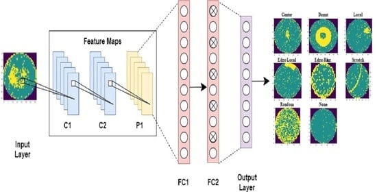
A simple CNN architecture is shown in Figure 2. The input layer receives the original images as the input. The convolutional layer is used to extract high-level features from the input images. The pooling layer reduces the sizes of particular features while maintaining the most important information. During the convolutional and pooling layers, the output is flattened to a 1D feature vector used as input for the fully connected layer, which connects the neurons on the previous layer with the neurons on the current layer. The final prediction results are calculated by the output layer.

3.2. Proposed Method Architecture

The architecture of the proposed DCNN-based prediction model for wafer map failure recognition is shown in Figure 3. In the proposed prediction model, the input image size is 224 × 224, the ReLU [37] is used as an activation function for each convolutional layer because of its efficiency, and the convolutional and max-pooling layers are used with 3 × 3 and 2 × 2 filter sizes, which are able to extract more detailed features while avoiding there being too many parameters. During the training process, the number of filters is increased with increasing depth of convolutional layers, which starts from 16 to 512 in the proposed DCNN prediction model. He’s uniform variance scaling initializer [39,40] and L2 regularization penalty (regularization parameter = 0.001) [41] are used in each convolutional layer to improve the training speed while avoiding the overfitting issue, and zero-padding [42] is used so that the output will have the same dimensions as the input. In addition, the proposed prediction model includes two fully connected layers with 512 feature maps after the convolutional and max-pooling layers, and a dropout rate of 0.5 is used to prevent overfitting [43] between the two fully connected layers. The Softmax activation function [38] is used in the output layer with 8 neurons to classify the input wafer map images with 8 classes, and the Adam optimizer [44] with a learning rate of 0.001 is used for weight optimization, because it is computationally efficient and can automatically decrease the learning rate [13]. The configuration parameters for the proposed DCNN-based prediction model are shown in Table 1.

3.3. Applied Machine Learning and Deep Learning Methods for Comparison

To evaluate the performance of our proposed DCNN model, we applied three widely used ML models—LR, RF, and GBDT—as well as several well-known DL models—VGGNet, ResNet, and EfficientNet—and compared their performance with our proposed prediction model. In the experiment, the representative VGG16, VGG19, ResNet50, ResNet101, and EfficientNetB0 were used. All applied ML and DL algorithms are introduced briefly in the following.
LR [19] is a popularly used statistical model in ML, and uses a logistic function to compress the output of linear equations in the classification problem to values between 0 and 1. The logistic function is used to describe the probabilities of possible outcomes. RF [20] is an ensemble learning approach for classification, regression, and other tasks. It constructs multiple decision trees that are then applied to different sub-samples of the original dataset during training, and then it selects the class with the maximum votes of the decision trees as the result during testing. Therefore, RF is able to deal with overfitting, improving the final performance. GBDT [21] is a powerful ML algorithm for building prediction models for both classification and regression problems. The models in GBDT are built sequentially, and each subsequent model tries to reduce the error obtained by the previous model. Finally, a strong model is produced that combines multiple decision tree-based weak prediction models and maximizes the prediction accuracy. VGG16 and VGG19 [22] are well-known VGGNet models, consisting of 16 and 19 weighted layers in the architectures. They were proposed by the Visual Geometry Group of Oxford University in 2015 and were able to obtain accurate classification performance on a very large image dataset. There are 13 convolution layers, 3 fully connected layers, 5 max-pooling layers, and 1 Softmax layer in VGG16, and 16 convolution layers, 3 fully connected layers, 5 max-pooling layers, and 1 Softmax layer in VGG19. In the VGG16 and VGG19 models, the number of filters increases with the increasing depth of convolution layers, which starts from 64 to 512 feature maps during training and includes two fully connected layers with 4096 neurons in each layer after the convolutional and max-pooling layers, and one output layer with the Softmax activation function and 8 neurons. ResNet [23] is a highly successful neural network that took first place in ImageNet Detection, ImageNet localization, Coco detection, and Coco segmentation at the ILSVRC and COCO 2015 competitions. ResNet50 and ResNet101 are residual network models that are 50 and 101 layers deep, respectively [23]. The ‘shortcut connection’, which can fit the input from the previous layer to the next layer without modifying the input, lies at the heart of the ResNet. In 2019, a novel CNN model called EfficientNet [24] was introduced, which is one of the most efficient CNN models, and is able to achieve state-of-the-art accuracy on ImageNet as well as common transfer learning tasks for image classification. The EfficientNet offers a range of models (B0 to B7) that are both efficient and accurate at multiple scales. We used the EfficientNetB0 in this paper. With a scaling heuristic, the efficiency-focused EfficientNetB0 model outperformed other models at each scale without requiring extensive grid searches for the hyperparameters.
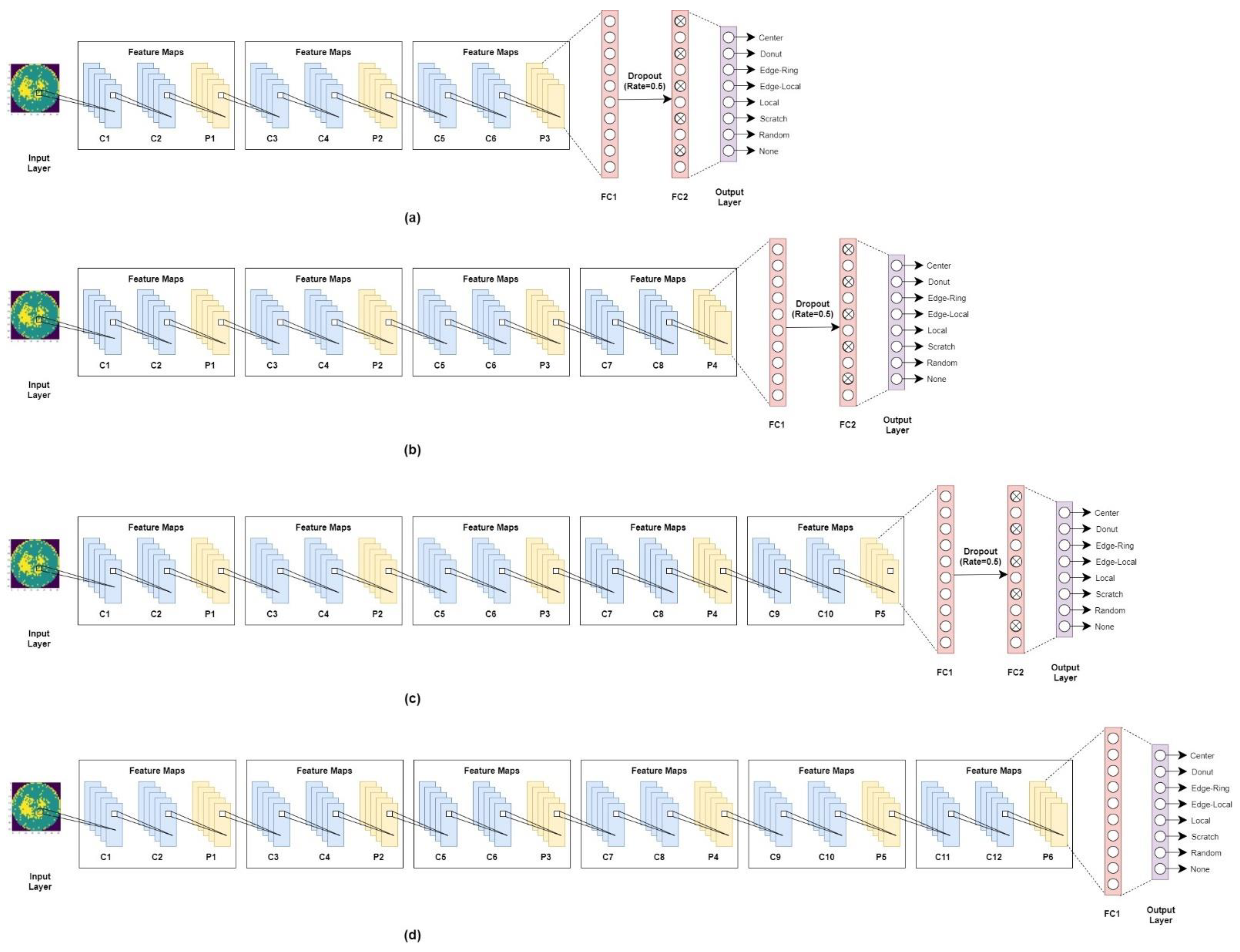
In addition, we also generated several models with less deep or much deeper layers of our proposed DCNN-based model, DCNN1, DCNN2, DCNN3, and DCNN4, which had very similar structures to that in the proposed method. The DCNN1 model includes 6 convolution layers, 3 max-pooling layers, 2 fully connected layers with 1 dropout layer (rate = 0.5), and 1 Softmax layer. In comparison to DCNN1, DCNN2 has two extra convolution layers and one more max-pooling layer, the DCNN3 has two additional convolution layers and one extra max-pooling layer than DCNN2, where the rest of the structures in the models are similar to each other. The DCNN4 has a similar structure to that of DCNN3, with the difference being that it only includes one fully connected layer, without a dropout layer after that. In each model, the number of filters increases as the number of convolutional layers becomes deeper, with (16, 32, and 64) filters in each feature map of DCNN1, (16, 32, 64, and 128) in each feature map of DCNN2, (16, 32, 64, 128, and 256) in each feature map of DCNN3, and (16, 32, 64, 128, 256, and 512) in each feature map of DCNN4. The configuration of the DCNN1, DCNN2, DCNN3, DCNN4-based prediction models is shown in Figure 4.

4. Experiments and Discussion

In this section, we introduce the data description and preprocessing for the experiment, and describe the performance measures for evaluating all of the ML and DL methods. After that, the implementation environment for the experiments and the experimental results are presented.

4.1. Data Description and Preprocessing

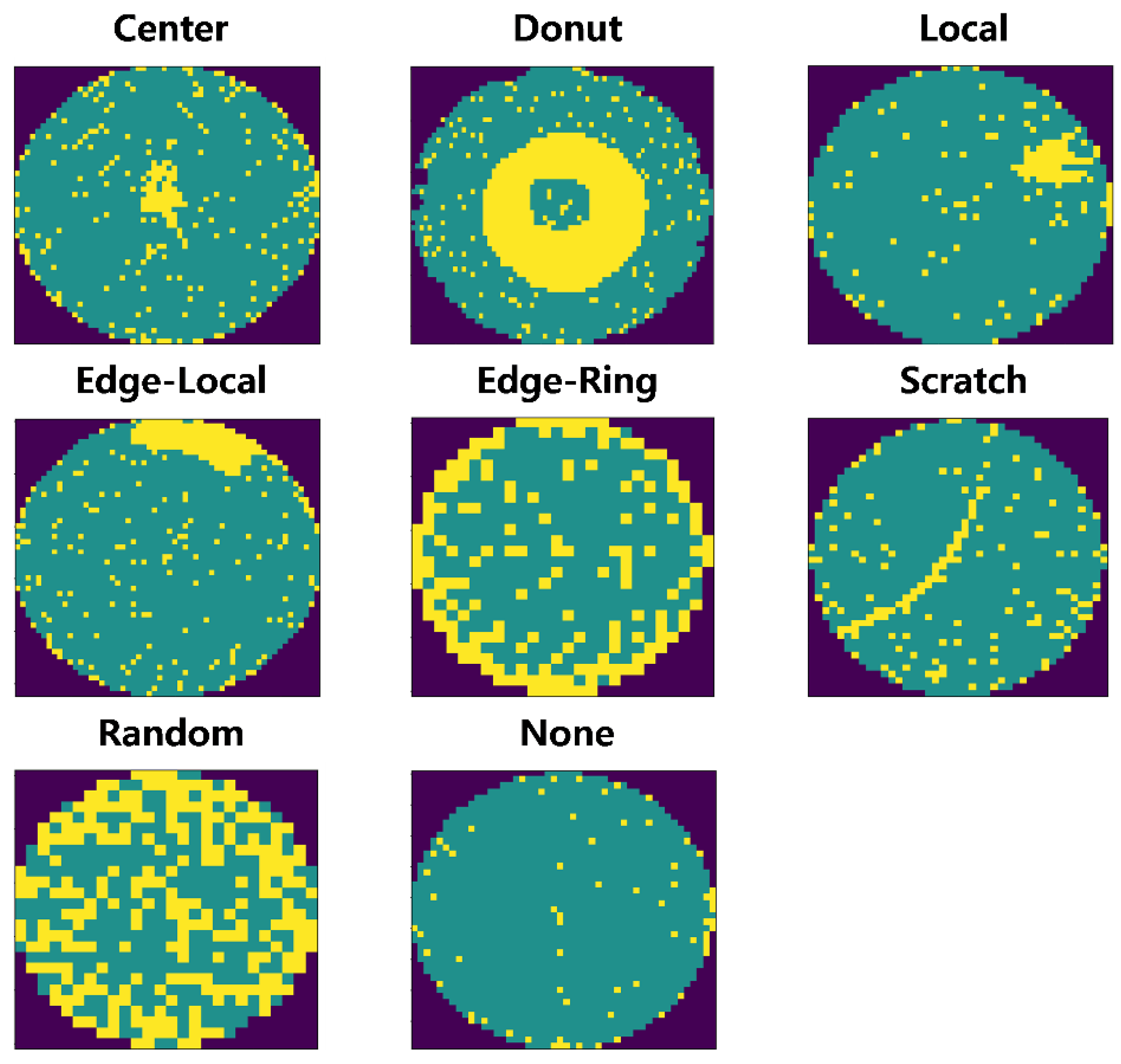
In this paper, we used the WM-811K dataset, which is a real-time semiconductor dataset including 811,457 wafer map images collected from 46,293 lots during the semiconductor fabrication process [3]. This is an open-source dataset that can be downloaded from the Multimedia Information Retrieval (MIR) laboratory website [25]. The dataset includes nine regular wafer map failure pattern types: Center, Donut, Local, Edge-Local, Edge-Ring, Scratch, Random, Near-Full, and None. The description of the dataset is shown in Table 2. There are a total of 172,950 labeled data in the original dataset of 811,457, with data for each failure class being highly imbalanced, especially the ‘Near-Full’ class, which only contains 149 images. Hence, we removed the ‘Near-Full’ class from our experimental data and focused on other eight wafer map failure pattern types. Figure 5 shows a typical example of eight wafer map failure types. We used random sampling to extract 500 images for the eight classes from the original dataset. For the final experimental dataset, a total of 4000 images belonging to the eight classes were used. Then the experimental dataset was split into training data, validation data, and test data, in proportions of 60%, 20% and 20%, respectively.

4.2. Performance Measures

To evaluate the performance of all ML- and DL-based prediction models for the recognition of wafer map failures, we use the accuracy, precision, recall, F1-score, and the area under the ROC curve (AUC) as the performance measures. The equations of the performance measures are shown in Equations (7) to (10) as follows:
A c c u r a c y = T P + T N T P + T N + F P + F N
P r e c i s i o n = T P T P + F P
R e c a l l = T P T P + F N
F 1 s c o r e = ( 2 R e c a l l P r e c i s i o n ) R e c a l l + P r e c i s i o n = ( 2 T P ) 2 T P + F P + F N
where the true positive, true negative, false positive, and false negative in the confusion matrix are shown as TP, TN, FP, and FN in abovementioned equations, respectively.

4.3. Implementation Environment

For the experiment, all implementations were analyzed on a PC with Intel Xeon CPU E5-2696 v5 @ 4.40 GHz, 512 GB RAM, and NVIDIA GeForce GTX 1080 24 GB. The ML- and DL-based prediction models were developed using the Tensorflow [45], Keras [46], and scikit-learn [47] packages in Jupyter Notebook [48] with Python (Version 3.6) [49].

4.4. Results of Prediction Models and Discussion

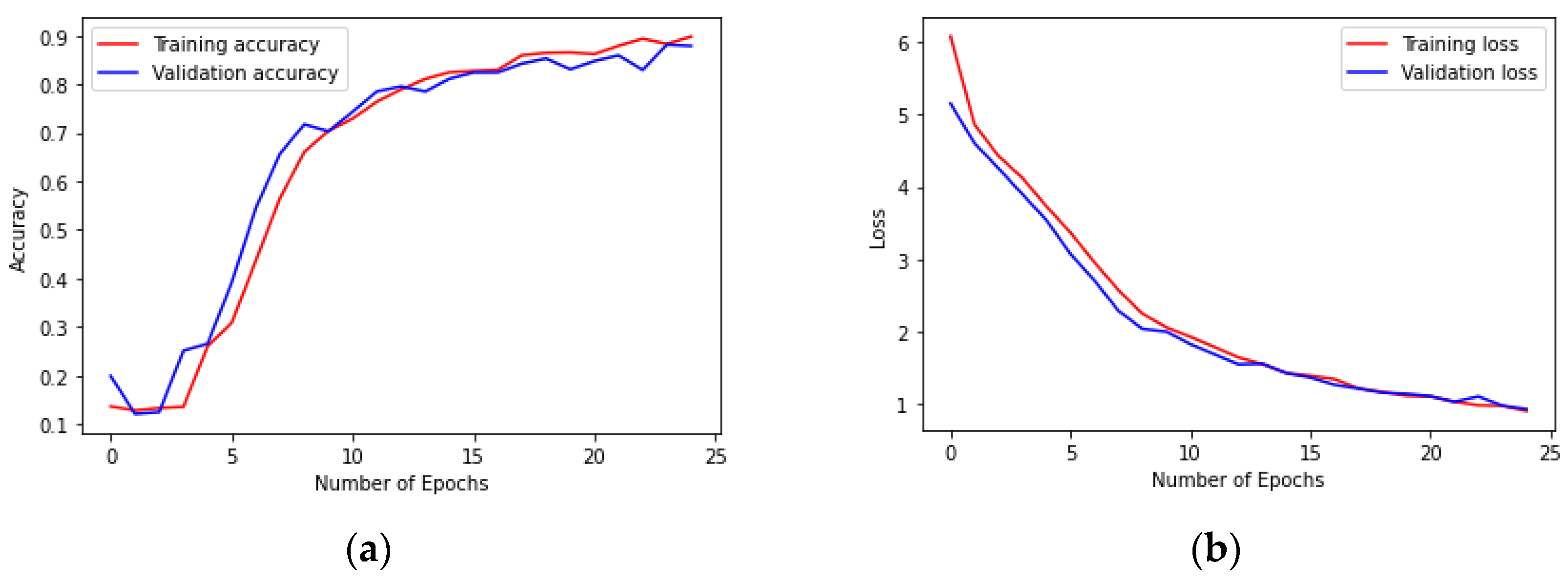
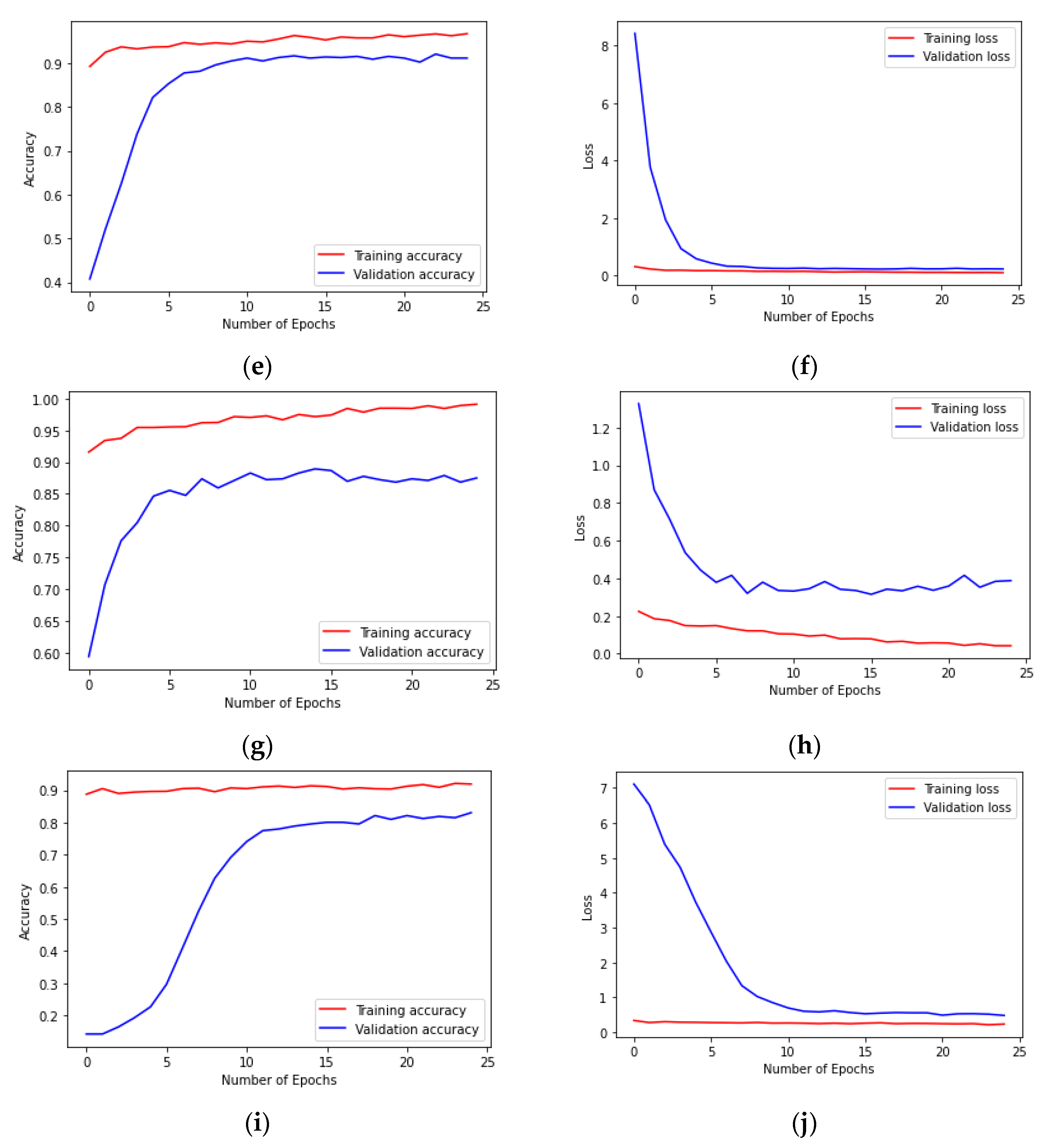
In the experiment, we proposed a DCNN prediction model for the recognition of wafer map failures. The performance of the proposed DCNN prediction model was compared with three popular ML-based algorithms—LR, RF, GBDT—and several well-known DL-based algorithms—VGGNet, ResNet, and EfficientNet. The batch size and epochs of the proposed DCNN and the other DL-based prediction models were designated as 96 and 25. The Adam optimizer was also used for the other predefined methods, because of its efficiency. We tested different learning rates for the VGG16-, VGG19-, ResNet50-, ResNet101-, and EfficientNetB0-based prediction models, and found that those five models could be trained accurately using the training and validation dataset when the learning rates were 0.0001, 0.0001, 0.000005, 0.00001, and 0.00001, respectively. The accuracy and loss learning curves of the proposed DCNN model, as well as the VGG16-, VGG19-, ResNet50-, ResNet101-, and EfficientNetB0-based prediction models are shown in Figure 6 and Figure 7.
Figure 6 shows the accuracy and loss learning curves of the proposed DCNN model during training and validation. In Figure 6a, it can be seen that the training accuracy of the proposed DCNN model dropped suddenly at the start of training, and then gradually increased over the next few training epochs, while the validation accuracy was monotonous during the first few epochs and then increased gradually. Figure 6b shows that the training and validation loss declined slowly across all epochs.
Figure 7 shows the learning curves of the compared DL-based prediction models—VGG16, VGG19, ResNet50, ResNet101, and EfficientNetB0. In Figure 7a,b, it can be seen that the training and validation accuracy of the VGG16 model increased swiftly at first and then increased gradually over several training epochs, whereas the training and validation loss of the VGG16 model decreased rapidly at the beginning and then decreased gradually over the following epochs. The training and validation learning curves of the VGG19 model were very similar to those of the VGG16 model, as shown in Figure 7c–f, which illustrate the learning curves of ResNet50, where the training accuracy slowly increased over time, and the validation accuracy increased quickly during the initial stage and then steadily increased over a series of training epochs, while the training loss exhibited little change, and the validation loss decreased rapidly at the beginning and then gradually decreased over the following epochs. The training and validation learning curves of ResNet101 and EfficientNetB0 in Figure 7g–j are very similar to those of ResNet50, where it can be seen that the validation accuracy increased faster than the training accuracy, and the range of validation loss changes was higher than the training loss. However, the ResNet50-, ResNet101-, and EfficientNetB0-based prediction models demonstrated a high probability of overfitting compared to the VGG16- and VGG19-based prediction models, because those three models had much deeper structures with much higher training accuracy and lower training loss.
Table 3 shows the results of the performance measures precision, recall, F1-score, and AUC of the proposed DCNN and the other compared models for all wafer failure pattern types—Center, Donut, Edge-Ring, Edge-Local, Local, Random, Scratch, and None. The results showed that the proposed DCNN-based prediction model was able to predict the wafer failure pattern types more accurately than the other ML- and DL-based models, possessing the best average recall, F1-score, and AUC, with values of 0.9919, 0.9766, and 0.999, respectively.
For each wafer failure patterns, the proposed DCNN model achieved the highest precision, F1-score, and AUC results, with values of 0.8511, 0.8081, 0.9726, respectively, for the ‘Local’ failure pattern types. Moreover, the proposed prediction model also achieved the highest recall and F1-score, with values of 0.9837 and 0.9641, 0.9419 and 0.9419, and 0.9901 and 0.9852, for the ‘Center’, ‘Donut’, and ‘Edge-Ring’ failure pattern types, respectively, as well as the highest recall and AUC results, with values of 1 and 1, for the ‘None’ failure pattern type. In addition, the VGG19 and ResNet50-based prediction models also achieved the best performance for the ‘None’ failure pattern type, with the highest values for precision, recall, F1-score, and AUC (1, 1, 1, and 1, respectively). In addition, the ResNet50 model obtained the highest precision and AUC results (0.9899 and 0.9999, respectively) for the ‘Edge-Ring’ failure pattern type. Additionally, the ResNet101 and EfficientNetB0 models received the best recall and AUC results (1 and 1, respectively) for the ‘None’ failure pattern type, which was also the same as that obtained by the proposed DCNN model. Furthermore, the GBDT model exhibited the highest precision, recall, F1-score, and AUC results (0.989, 1, 0.9945, and 0.9999, respectively) for ‘Random’, and the best precision and AUC results (0.9664 and 0.9988, respectively) for the ‘Center’ failure pattern types. The RF model achieved the best performance for the ‘Edge-Local’ failure pattern type, with the highest recall, F1-score, and AUC results (0.9802, 0.9754, and 0.9997, respectively), and the ‘Random’ and ‘Scratch’ failure pattern types, with the highest values of recall and AUC (1 and 0.9999, respectively), and precision and AUC (0.9639 and 0.9974, respectively).
However, the highest F1-score achieved by the proposed DCNN model for the ‘Local’ failure pattern type was 0.8081, which is not a satisfactory result when compared to the results obtained for the other wafer failure pattern types. A possible reason for this problem is that there was noise in the original image dataset, or that the experimental dataset was extracted by random sampling.
The overall performance comparison results of different prediction models are shown in Table 4. As can be seen from the results, the performance of the proposed DCNN-based prediction model outperformed the other eight prediction models in terms of precision, recall, F1-score, AUC, and accuracy, with values of 0.9381, 0.9379, 0.9376, 0.9933, and 0.9375, respectively, while the ResNet50-based prediction model exhibited an equivalent performance in AUC of 0.9933.
It can also be seen that the overall results for all prediction models mentioned in Table 4 decreased with respect to the performance of each class mentioned in Table 3. This may have been a result of the significantly lower performance of the ‘Local’ failure pattern type compared to the other failure types. Additionally, the results also showed that the DL-based techniques exhibited improved performances for the recognition of wafer map failure pattern types compared to the ML-based methods when comparing the average and overall performances of all ML- and DL-based prediction models.
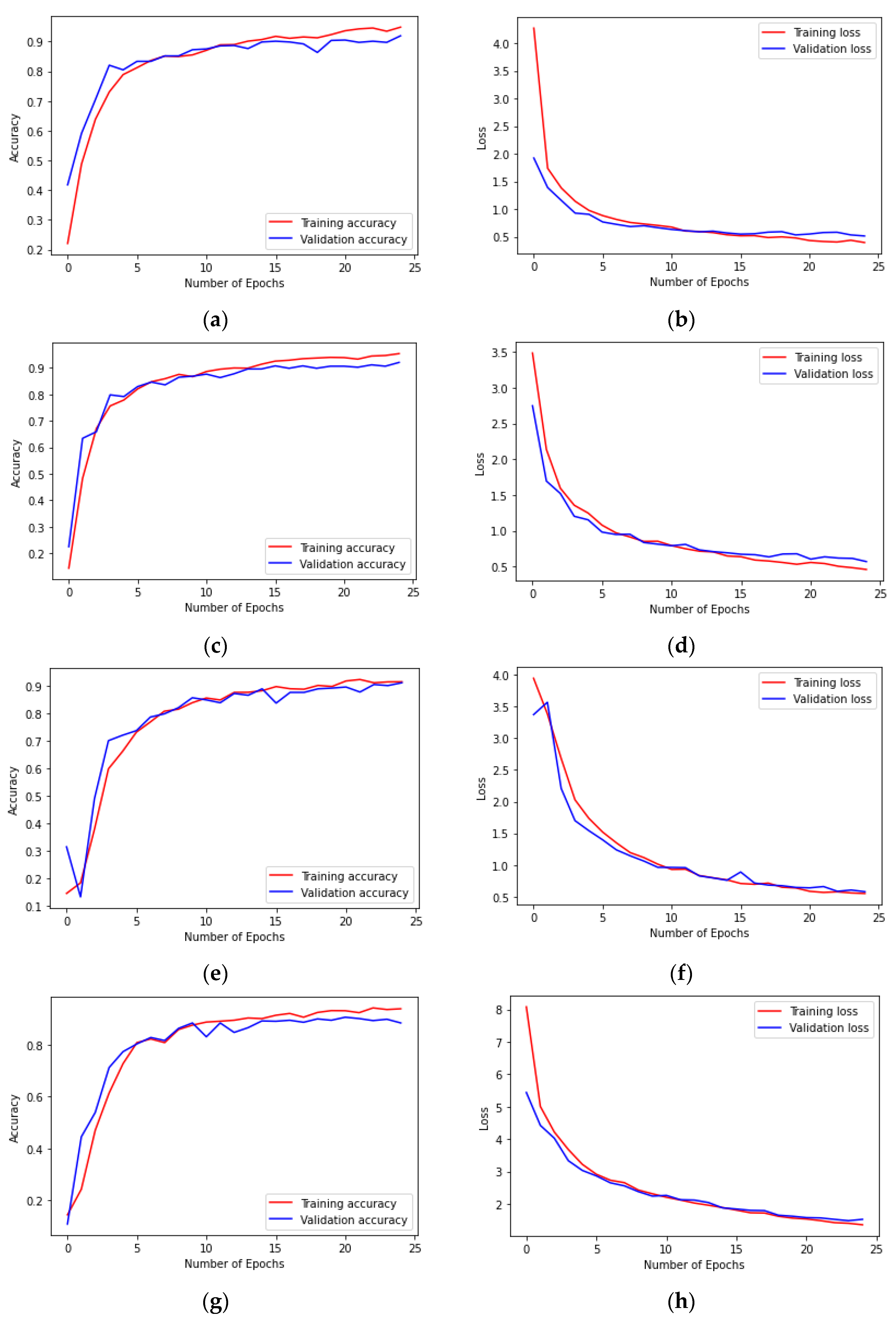
We also developed several DCNN-based models with fewer or much deeper layers, denoted as DCNN1, DCNN2, DCNN3, and DCNN4, which had very similar structures to the proposed method. To develop these models, the Adam optimizer was also used in the experiments due to its efficiency. We tested different learning rates for the DCNN1-, DCNN2-, DCNN3-, and DCNN4-based prediction models, and found that the optimal learning rate was 0.001 for all four models during training and validation. Figure 8 illustrates how the DCNN1-, DCNN2-, DCNN3-, and DCNN4-based prediction models performed in terms of accuracy and loss learning curves.
In Figure 8a, it can be seen that the training and validation accuracy of the DCNN1 model increased suddenly during the first several epochs of training, and then gradually increased with increasing number of epochs; Figure 8b shows that the training loss of the DCNN1 model dropped rapidly during the initial stage and then declined slowly, while validation loss decreased gradually over all epochs. The accuracy and loss learning curves of the DCNN2 and DCNN4 models are similar to those of DCNN1, as shown in Figure 8c,d,g,h; nonetheless, the validation loss of DCNN2 in Figure 8c dropped quickly at first, and then declined rapidly over the following epochs. Figure 8e,f reveal the accuracy and loss learning curves of the DCNN3 model in training and validation. In Figure 8e, it can be seen that the training accuracy of the DCNN3 model increased slowly during the first stage of training, and then swiftly improved for several epochs and then increased steadily until the end; the validation accuracy suddenly decreased at the beginning and then rapidly increased over the next few training epochs, before increasing gradually. The behaviors of the loss learning curves in training and validation were the opposite of those of the accuracy learning curves during the training and validation, as shown in Figure 8f, showing that the training loss initially declined quickly, before decreasing steadily, while the validation loss increased in first epoch and then rapidly dropped before gradually declining with increasing numbers of epochs.
Table 5 shows the results of the overall performance comparison of the DCNN prediction models with different structures like DCNN1, DCNN2, DCNN3, and DCNN4, with the results showing that the proposed DCNN-based method achieved the best performance with the highest values for precision, recall, F1-score, AUC, and accuracy, at 0.9381, 0.9379, 0.9376, 0.9933, and 0.9375, respectively, outperforming the other four models.

5. Conclusions

This paper presents a DL-based convolutional neural network (DCNN) prediction model for the recognition of wafer map failure types based on the real-time wafer map image dataset. The performance of the proposed prediction model was compared with three state-of-the-art ML-based prediction models—LR, RF, GBDT—and several well-known DL models—VGGNet, ResNet, and EfficientNet. Consequently, our findings indicated that the proposed prediction model achieved the best performance among the selected popular ML- and DL-based models. In addition, the proposed prediction model outperformed the other models with fewer or much deeper layers. However, the ‘Local’ failure pattern type was recognized less accurately than other failure pattern types. Therefore, we will consider generating a more robust model using more image datasets and removing the noise in the dataset for experiments in the future. Moreover, the rule-based fuzzy classifier [50,51] has a unique advantage with respect to interpreting the classification, which can be considered in future work, because the ML- and DL-based techniques have a weakness with respect to interpretability.

Limitations

However, there are a number of limitations to this paper. First, there is a high probability that the experimental image dataset was not represented in the raw dataset, because it was extracted by a random sampling technique. Second, both the ML- and DL-based models were less able to predict the ‘Local’ failure type accurately (F1-score = 0.8081 with the proposed DCNN) than they were the other seven wafer map failure pattern types. Third, the ResNet50, ResNet101, and EfficientNetB0-based prediction models may not have been generated properly in this experiment, because they had deep structures and were trained using large datasets, while the size of the training dataset was small in this experiment.

Author Contributions

Conceptualization, H.Z. and J.Y.L.; methodology, H.Z.; software, H.Z.; validation, H.Z., S.W.A.S. and S.H.S.; formal analysis, H.Z.; investigation, H.Z., S.W.A.S. and S.H.S.; resources, H.Z. and J.Y.L.; data curation, H.Z. and J.Y.L.; writing—original draft preparation, H.Z.; writing—review and editing, H.Z., S.W.A.S., S.H.S. and J.Y.L.; visualization, H.Z., S.W.A.S. and S.H.S.; supervision, J.Y.L.; project administration, J.Y.L.; funding acquisition, J.Y.L. All authors have read and agreed to the published version of the manuscript.

Funding

This research was funded by Korea Institute for Advancement of Technology (KIAT) grant through the Korea Government by Ministry of Trade, Industry and Energy (MOTIE) (No. N0002429), in part by Basic Science Research Program through the National Research Foundation of Korea (NRF) by the Ministry of Education (No.2017R1D1A1A02018718), and in part by the Ministry of Science and ICT (MSIT), Korea, through the Grand Information Technology Research Center support program supervised by the Institute for Information and Communications Technology Planning and Evaluation (IITP) (IITP-2021-2020-0-01462).

Institutional Review Board Statement

Not applicable.

Informed Consent Statement

Not applicable.

Data Availability Statement

The data is an open-source dataset and can be downloaded in the MIR Corpora (Available online: http://mirlab.org/dataSet/public/) (accessed on 18 October 2021).

Conflicts of Interest

The authors declare no conflict of interest.

References

  1. Wang, R.; Chen, N. Defect pattern recognition on wafers using convolutional neural networks. Qual. Reliab. Eng. Int. 2020, 36, 1245–1257. [Google Scholar] [CrossRef]
  2. Yuan, T.; Kuo, W.; Bae, S.J. Detection of spatial defect patterns generated in semiconductor fabrication processes. IEEE Trans. Semicond. Manuf. 2011, 24, 392–403. [Google Scholar] [CrossRef]
  3. Wu, M.J.; Jang, J.S.R.; Chen, J.L. Wafer map failure pattern recognition and similarity ranking for large-scale data sets. IEEE Trans. Semicond. Manuf. 2014, 28, 1–12. [Google Scholar] [CrossRef]
  4. Piao, M.; Jin, C.H.; Lee, J.Y.; Byun, J.Y. Decision tree ensemble-based wafer map failure pattern recognition based on radon transform-based features. IEEE Trans. Semicond. Manuf. 2018, 31, 250–257. [Google Scholar] [CrossRef]
  5. Jin, C.H.; Na, H.J.; Piao, M.; Pok, G.; Ryu, K.H. A novel DBSCAN-based defect pattern detection and classification framework for wafer bin map. IEEE Trans. Semicond. Manuf. 2019, 32, 286–292. [Google Scholar] [CrossRef]
  6. Drozda-Freeman, A.; McIntyre, M.; Retersdorf, M.; Wooten, C.; Song, X.; Hesse, A. The application and use of an automated spatial pattern recognition (SPR) system in the identification and solving of yield issues in semiconductor manufacturing. In Proceedings of the 2007 IEEE/SEMI Advanced Semiconductor Manufacturing Conference, Stresa, Italy, 11–12 June 2007; pp. 302–305. [Google Scholar] [CrossRef]
  7. He, Q.P.; Wang, J. Fault detection using the k-nearest neighbor rule for semiconductor manufacturing processes. IEEE Trans. Semicond. Manuf. 2007, 20, 345–354. [Google Scholar] [CrossRef]
  8. Saqlain, M.; Jargalsaikhan, B.; Lee, J.Y. A voting ensemble classifier for wafer map defect patterns identification in semiconductor manufacturing. IEEE Trans. Semicond. Manuf. 2019, 32, 171–182. [Google Scholar] [CrossRef]
  9. Saqlain, M.; Abbas, Q.; Lee, J.Y. A deep convolutional neural network for wafer defect identification on an imbalanced dataset in semiconductor manufacturing processes. IEEE Trans. Semicond. Manuf. 2020, 33, 436–444. [Google Scholar] [CrossRef]
  10. Hsu, S.C.; Chien, C.F. Hybrid data mining approach for pattern extraction from wafer bin map to improve yield in semiconductor manufacturing. Int. J. Prod. Econ. 2007, 107, 88–103. [Google Scholar] [CrossRef]
  11. Choi, G.; Kim, S.H.; Ha, C.; Bae, S.J. Multi-step ART1 algorithm for recognition of defect patterns on semiconductor wafers. Int. J. Prod. Res. 2012, 50, 3274–3287. [Google Scholar] [CrossRef]
  12. Rawat, W.; Wang, Z. Deep convolutional neural networks for image classification: A comprehensive review. Neural Comput. 2017, 29, 2352–2449. [Google Scholar] [CrossRef]
  13. Li, Z.; Liu, F.; Yang, W.; Peng, S.; Zhou, J. A survey of convolutional neural networks: Analysis, applications, and prospects. IEEE Trans. Neural Netw. Learn. Syst. 2021, 1–21. [Google Scholar] [CrossRef]
  14. Ullah, I.; Manzo, M.; Shah, M.; Madden, M. Graph Convolutional Networks: Analysis, improvements and results. arXiv 2019, arXiv:1912.09592. [Google Scholar]
  15. Dimitriou, N.; Leontaris, L.; Vafeiadis, T.; Ioannidis, D.; Wotherspoon, T.; Tinker, G.; Tzovaras, D. Fault diagnosis in microelectronics attachment via deep learning analysis of 3-D laser scans. IEEE Trans. Ind. Electron. 2019, 67, 5748–5757. [Google Scholar] [CrossRef] [Green Version]
  16. Dimitriou, N.; Leontaris, L.; Vafeiadis, T.; Ioannidis, D.; Wotherspoon, T.; Tinker, G.; Tzovaras, D. A deep learning framework for simulation and defect prediction applied in microelectronics. Simul. Model. Pract. Theory 2020, 100, 102063. [Google Scholar] [CrossRef] [Green Version]
  17. Nakazawa, T.; Kulkarni, D.V. Wafer map defect pattern classification and image retrieval using convolutional neural network. IEEE Trans. Semicond. Manuf. 2018, 31, 309–314. [Google Scholar] [CrossRef]
  18. Shon, H.S.; Batbaatar, E.; Cho, W.S.; Choi, S.G. Unsupervised Pre-Training of Imbalanced Data for Identification of Wafer Map Defect Patterns. IEEE Access 2021, 9, 52352–52363. [Google Scholar] [CrossRef]
  19. Bagley, S.C.; White, H.; Golomb, B.A. Logistic regression in the medical literature: Standards for use and reporting, with particular attention to one medical domain. J. Clin. Epidemiol. 2001, 54, 979–985. [Google Scholar] [CrossRef]
  20. Breiman, L. Random forests. Mach. Learn. 2001, 45, 5–32. [Google Scholar] [CrossRef] [Green Version]
  21. Friedman, J.H. Greedy boosting approximation: A gradient boosting machine. Ann. Stat. 2001, 29, 1189–1232. [Google Scholar] [CrossRef]
  22. Simonyan, K.; Zisserman, A. Very deep convolutional networks for large-scale image recognition. arXiv 2014, arXiv:1409.1556. [Google Scholar]
  23. He, K.; Zhang, X.; Ren, S.; Sun, J. Deep residual learning for image recognition. In Proceedings of the IEEE Conference on Computer Vision and Pattern Recognition, Las Vegas, NV, USA, 27–30 June 2016; pp. 770–778. [Google Scholar] [CrossRef] [Green Version]
  24. Tan, M.; Le, Q. Efficientnet: Rethinking model scaling for convolutional neural networks. In Proceedings of the 36th International Conference on Machine Learning, Long Beach, CA, USA, 9–15 June 2019; PMLR 97. pp. 6105–6114. [Google Scholar]
  25. Mirlab.org. MIR Corpora. Available online: http://mirlab.org/dataSet/public/ (accessed on 6 October 2021).
  26. He, Q.P.; Wang, J. Principal component based k-nearest-neighbor rule for semiconductor process fault detection. In Proceedings of the 2008 American Control Conference, Seattle, WA, USA, 11–13 June 2008; pp. 1606–1611. [Google Scholar] [CrossRef]
  27. Chao, L.C.; Tong, L.I. Wafer defect pattern recognition by multi-class support vector machines by using a novel defect cluster index. Expert Syst. Appl. 2009, 36, 10158–10167. [Google Scholar] [CrossRef]
  28. Kang, S.; Cho, S.; An, D.; Rim, J. Using wafer map features to better predict die-level failures in final test. IEEE Trans. Semicond. Manuf. 2015, 28, 431–437. [Google Scholar] [CrossRef]
  29. Kim, D.; Kang, P.; Cho, S.; Lee, H.J.; Doh, S. Machine learning-based novelty detection for faulty wafer detection in semiconductor manufacturing. Expert Syst. Appl. 2012, 39, 4075–4083. [Google Scholar] [CrossRef]
  30. Jizat, J.A.M.; Majeed, A.P.A.; Nasir, A.F.A.; Taha, Z.; Yuen, E. Evaluation of the machine learning classifier in wafer defects classification. ICT Express 2021, 1–5. [Google Scholar] [CrossRef]
  31. Cheon, S.; Lee, H.; Kim, C.O.; Lee, S.H. Convolutional neural network for wafer surface defect classification and the detection of unknown defect class. IEEE Trans. Semicond. Manuf. 2019, 32, 163–170. [Google Scholar] [CrossRef]
  32. Kim, J.; Kim, H.; Park, J.; Mo, K.; Kang, P. Bin2Vec: A better wafer bin map coloring scheme for comprehensible visualization and effective bad wafer classification. Appl. Sci. 2019, 9, 597. [Google Scholar] [CrossRef] [Green Version]
  33. Nakazawa, T.; Kulkarni, D.V. Anomaly detection and segmentation for wafer defect patterns using deep convolutional encoder–decoder neural network architectures in semiconductor manufacturing. IEEE Trans. Semicond. Manuf. 2019, 32, 250–256. [Google Scholar] [CrossRef]
  34. Alawieh, M.B.; Boning, D.; Pan, D.Z. Wafer map defect patterns classification using deep selective learning. In Proceedings of the 2020 57th ACM/IEEE Design Automation Conference (DAC), San Francisco, CA, USA, 20–24 July 2020; pp. 1–6. [Google Scholar] [CrossRef]
  35. LeCun, Y.; Boser, B.; Denker, J.S.; Henderson, D.; Howard, R.E.; Hubbard, W.; Jackel, L.D. Backpropagation applied to handwritten zip code recognition. Neural Comput. 1989, 1, 541–551. [Google Scholar] [CrossRef]
  36. Chen, X.; Chai, Q.; Lin, N.; Li, X.; Wang, W. 1D convolutional neural network for the discrimination of aristolochic acids and their analogues based on near-infrared spectroscopy. Anal. Methods 2019, 11, 5118–5125. [Google Scholar] [CrossRef]
  37. Nair, V.; Hinton, G.E. Rectified linear units improve restricted boltzmann machines. In Proceedings of the 27th International Conference on International Conference on Machine Learning, Haifa, Israel, 21–24 June 2010; pp. 807–814. [Google Scholar]
  38. Sharma, S.; Sharma, S. Activation functions in neural networks. Towards Data Sci. 2017, 6, 310–316. [Google Scholar]
  39. He, K.; Zhang, X.; Ren, S.; Sun, J. Delving deep into rectifiers: Surpassing human-level performance on imagenet classification. In Proceedings of the IEEE international conference on computer vision, Santiago, Chile, 7–13 December 2015; pp. 1026–1034. [Google Scholar] [CrossRef] [Green Version]
  40. Yam, J.Y.; Chow, T.W. A weight initialization method for improving training speed in feedforward neural network. Neurocomputing 2000, 30, 219–232. [Google Scholar] [CrossRef]
  41. Bilgic, B.; Chatnuntawech, I.; Fan, A.P.; Setsompop, K.; Cauley, S.F.; Wald, L.L.; Adalsteinsson, E. Fast image reconstruction with L2--regularization. J. Magn. Reson. Imaging 2014, 40, 181–191. [Google Scholar] [CrossRef] [Green Version]
  42. Albawi, S.; Mohammed, T.A.; Al-Zawi, S. Understanding of a convolutional neural network. In Proceedings of the 2017 International Conference on Engineering and Technology (ICET), Antalya, Turkey, 21–23 August 2017; IEEE: Piscataway, NJ, USA; pp. 1–6. [Google Scholar]
  43. Srivastava, N.; Hinton, G.; Krizhevsky, A.; Sutskever, I.; Salakhutdinov, R. Dropout: A simple way to prevent neural networks from overfitting. J. Mach. Learn. Res. 2014, 15, 1929–1958. [Google Scholar]
  44. Kingma, D.P.; Ba, J. Adam: A method for stochastic optimization. arXiv 2014, arXiv:1412.6980. [Google Scholar]
  45. Abadi, M.; Agarwal, A.; Barham, P.; Brevdo, E.; Chen, Z.; Citro, C.; Corrado, G.S.; Davis, A.; Dean, J.; Devin, M.; et al. Tensorflow: Large-scale machine learning on heterogeneous distributed systems. arXiv 2016, arXiv:1603.04467. [Google Scholar]
  46. Keras.io. Keras Documentation. Available online: https://keras.io/ (accessed on 6 October 2021).
  47. Pedregosa, F.; Varoquaux, G.; Gramfort, A.; Michel, V.; Thirion, B.; Grisel, O.; Blondel, M.; Prettenhofer, P.; Weiss, R.; Dubourg, V.; et al. Scikit-learn: Machine learning in Python. J. Mach. Learn. Res. 2011, 12, 2825–2830. [Google Scholar]
  48. Jupyter.org. Project Jupyter. Available online: http://jupyter.org/ (accessed on 6 October 2021).
  49. Van Rossum, G.; Drake, F.L. Python 3 Reference Manual; CreateSpace: Scotts Valley, CA, USA, 2009. [Google Scholar]
  50. Pellicano, D.; Palamara, I.; Cacciola, M.; Calcagno, S.; Versaci, M.; Morabito, F.C. Fuzzy similarity measures for detection and classification of defects in CFRP. IEEE Trans. Ultrason. Ferroelectr. Freq. Control 2013, 60, 1917–1927. [Google Scholar] [CrossRef] [PubMed]
  51. Bardamova, M.; Konev, A.; Hodashinsky, I.; Shelupanov, A. A fuzzy classifier with feature selection based on the gravitational search algorithm. Symmetry 2018, 10, 609. [Google Scholar] [CrossRef] [Green Version]
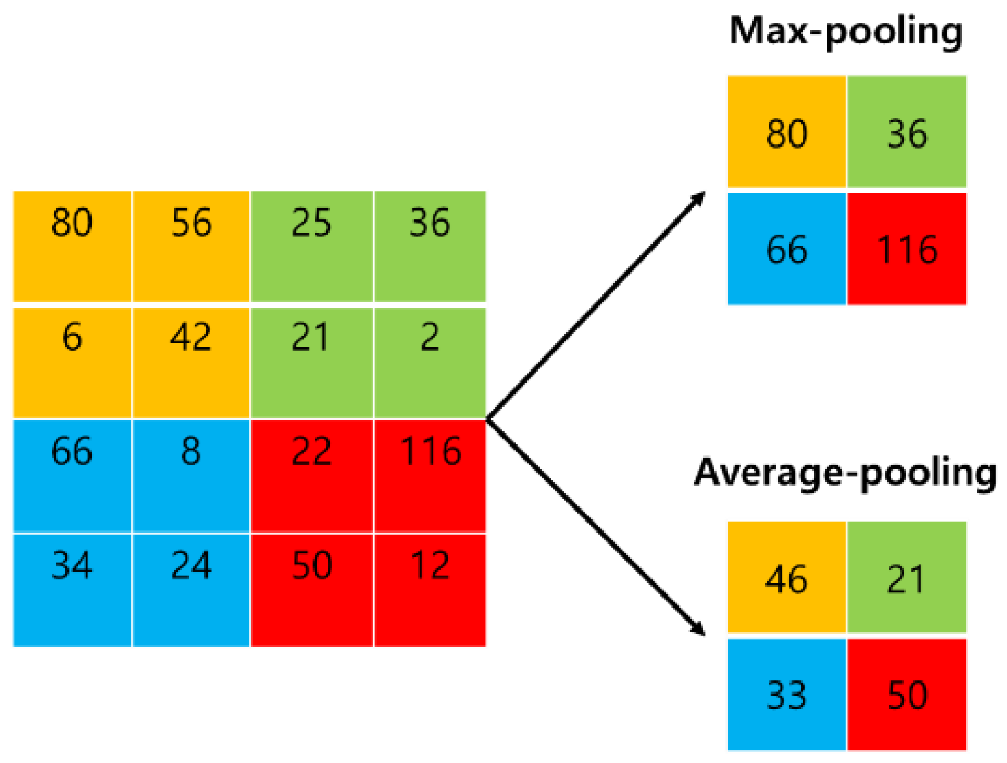
Figure 1. Two common types of pooling method.
Applsci 11 09769 g001
Figure 2. A simple CNN architecture.
Applsci 11 09769 g002
Figure 3. The architecture of the proposed DCNN-based prediction model for wafer map failure recognition. Note: C denotes the convolutional layer, P the pooling layer, and FC the fully connected layer.
Applsci 11 09769 g003
Figure 4. The configuration of the (a) DCNN1, (b) DCNN2, (c) DCNN3, (d) and DCNN4-based prediction models. Note: C denotes the convolutional layer, P the pooling layer, and FC the fully connected layer.
Applsci 11 09769 g004
Figure 5. Typical examples of eight wafer map failure types.
Applsci 11 09769 g005
Figure 6. The learning curves of the proposed prediction model: (a) the accuracy learning curves of DCNN; (b) the loss learning curves of DCNN.
Applsci 11 09769 g006
Figure 7. The learning curves of the compared DL-based prediction models: (a) the accuracy learning curves of VGG16; (b) the loss learning curves of VGG16; (c) the accuracy learning curves of VGG19; (d) the loss learning curves of VGG19; (e) the accuracy learning curves of ResNet50; (f) the loss learning curves of ResNet50; (g) the accuracy learning curves of ResNet101; (h) the loss learning curves of ResNet101; (i) the accuracy learning curves of EfficientNetB0; (j) the loss learning curves of EfficientNetB0.
Applsci 11 09769 g007aApplsci 11 09769 g007b
Figure 8. The learning curves of the compared DL-based prediction models: (a) the accuracy learning curves of DCNN1; (b) the loss learning curves of DCNN1; (c) the accuracy learning curves of DCNN2; (d) the loss learning curves of DCNN2; (e) the accuracy learning curves of DCNN3; (f) the loss learning curves of DCNN3; (g) the accuracy learning curves of DCNN4; (h) the loss learning curves of DCNN4.
Applsci 11 09769 g008
Table 1. The configuration parameters of the proposed DCNN-based prediction model.
LayerDetailed Parameters
Input layerSize (224 × 224)
C116 3 × 3 2D convolutional layer (Relu)
C216 3 × 3 2D convolutional layer (Relu)
P1Max pooling layer 2 × 2
C332 3 × 3 2D convolutional layer (Relu)
C432 3 × 3 2D convolutional layer (Relu)
P2Max pooling layer 2 × 2
C564 3 × 3 2D convolutional layer (Relu)
C664 3 × 3 2D convolutional layer (Relu)
P3Max pooling layer 2 × 2
C7128 3 × 3 2D convolutional layer (Relu)
C8128 3 × 3 2D convolutional layer (Relu)
P4Max pooling layer 2 × 2
C9256 3 × 3 2D convolutional layer (Relu)
C10256 3 × 3 2D convolutional layer (Relu)
P5Max pooling layer 2 × 2
C11512 3 × 3 2D convolutional layer (Relu)
C12512 3 × 3 2D convolutional layer (Relu)
P6Max pooling layer 2 × 2
Flatten
FC1Fully connected layer 512 (Relu)
Dropout layerDropout (rate = 0.5)
FC2Fully connected layer 512 (Relu)
Output layerOutput layer 8 (Softmax)
Table 2. Data description.
TypeCount
Center4296 (2.5%)
Donut555 (0.3%)
Local3597 (2.1%)
Edge-Local5199 (3.0%)
Edge-Ring9682 (5.6%)
Scratch1194 (0.7%)
Random866 (0.5%)
Near-Full149 (0.1%)
None147,431 (85.2%)
Total172,950 (100%)
Table 3. Performance comparison results of multi-class wafer map image classification.
MethodClassifierMeasureCenterDonutEdge-RingEdge-LocalLocalRandomScratchNoneAverage
ML-based MethodsLRPrecision0.95730.90240.76030.98990.72280.97830.93260.78790.8726
Recall0.91060.86050.82140.97030.701910.91210.83870.8747
F1-score0.93330.8810.78970.980.71220.9890.92220.81250.8729
AUC0.99710.98620.97140.99920.96120.99930.99670.97720.9872
RFPrecision0.95120.90120.77590.97060.70370.97830.96390.93160.9414
Recall0.95120.84880.80360.98020.730810.87910.84950.9004
F1-score0.95120.87430.78950.97540.7170.9890.91950.84040.8958
AUC0.99830.98710.97650.99970.95230.99990.99740.98460.9915
GBDTPrecision0.96640.88890.79820.980.70540.9890.96250.79610.8813
Recall0.9350.83720.81250.97030.759610.84620.88170.9084
F1-score0.95040.86230.80530.97510.73150.99450.90060.83670.8936
AUC0.99880.97740.97520.99970.96860.99990.99690.9870.9929
DL-based MethodsVGG16Precision0.95080.95240.97060.82860.6990.95560.78640.9780.9644
Recall0.94310.93020.98020.77680.69230.94510.8710.98890.966
F1-score0.94690.94120.97540.80180.69570.95030.82650.98340.9652
AUC0.99820.99840.99960.98090.96510.99590.98810.99990.999
VGG19Precision0.88970.94520.95240.91110.72970.97670.807310.9449
Recall0.98370.80230.99010.73210.77880.92310.946210.9919
F1-score0.93440.86790.97090.81190.75350.94920.871310.9672
AUC0.99790.99530.99940.97650.95850.99790.992810.999
ResNet50Precision0.96520.96250.98990.88390.71540.98850.872310.9826
Recall0.90240.89530.97030.88390.84620.95410.881710.9512
F1-score0.93280.92770.980.88390.77530.96630.87710.9664
AUC0.99730.99730.99990.99030.96770.99970.992810.9987
ResNet101Precision0.90620.8370.97090.72220.74390.9570.84710.9890.9476
Recall0.94310.89530.99010.81250.58650.9780.774210.9716
F1-score0.92430.86520.98040.76470.65590.96740.8090.99450.9594
AUC0.99370.9920.99790.9760.95630.99950.984610.9969
EfficientNetB0Precision0.83330.77780.970.80370.6250.98680.78650.97830.9058
Recall0.85370.8140.96040.76790.72120.82420.752710.9269
F1-score0.84340.79550.96520.78540.66960.89820.76920.9890.9162
AUC0.97440.97920.99870.98050.95080.99790.971710.9872
Proposed DCNNPrecision0.94530.94190.98040.90520.85110.98880.9140.97830.9618
Recall0.98370.94190.99010.93750.76920.9670.91410.9919
F1-score0.96410.94190.98520.92110.80810.97780.9140.9890.9766
AUC0.99790.9980.99830.98530.97260.99960.993610.999
Note: The best results are shown in bold.
Table 4. Overall performance comparison results of different prediction models.
ClassifierPrecisionRecallF1-scoreAUCAccuracy
LR0.87890.87690.87750.99060.875
RF0.88450.88040.8820.9910.88
GBDT0.88580.88030.8820.99140.88
VGG160.89020.89090.89020.9910.8875
VGG190.90150.89460.89490.98970.8938
ResNet500.92220.91560.91790.99330.9137
ResNet1010.87170.87250.87020.98790.87
EfficientNetB00.84520.83670.83940.98220.835
Proposed DCNN 0.93810.93790.93760.99330.9375
Note: The best results are shown in bold.
Table 5. Overall performance comparison results of the DCNN-based prediction models with different structures.
ClassifierPrecisionRecallF1-scoreAUCAccuracy
DCNN10.90320.89030.89420.99120.8925
DCNN20.91040.91270.91130.99080.91
DCNN30.90370.90230.90060.99010.9012
DCNN40.86730.87460.8670.98670.8688
Proposed DCNN 0.93810.93790.93760.99330.9375
Note: The best results are shown in bold.
Publisher’s Note: MDPI stays neutral with regard to jurisdictional claims in published maps and institutional affiliations.