
A Deep Convolutional Neural Network-Based Multi-Class Image Classification for Automatic Wafer Map Failure Recognition in Semiconductor Manufacturing


Abstract
:
1. Introduction
- The whole experiment was conducted using the real-time wafer map dataset WM-811K [25].
- Using the random sampling technique, we were able to extract the representative image data of different wafer map failure pattern types, improving the efficiency of the experiment, and reducing the temporal and spatial complexity without the use of large-scale raw wafer map data.
- A deep learning-based DCNN model is proposed for the automatic recognition of wafer map failure pattern types.
- The experimental results demonstrate that the proposed model enhances the accuracy of the recognition of wafer map failure pattern types compared to other popular ML- and DL-based models.
2. Literature Review
3. Methodology
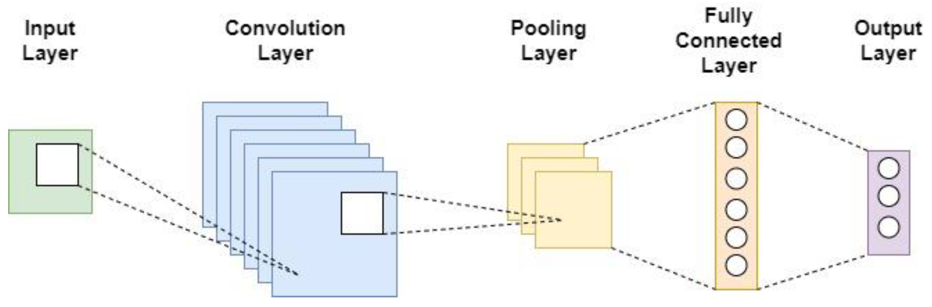
3.1. Convolutional Neural Network
- Input layer
- Convolutional layer
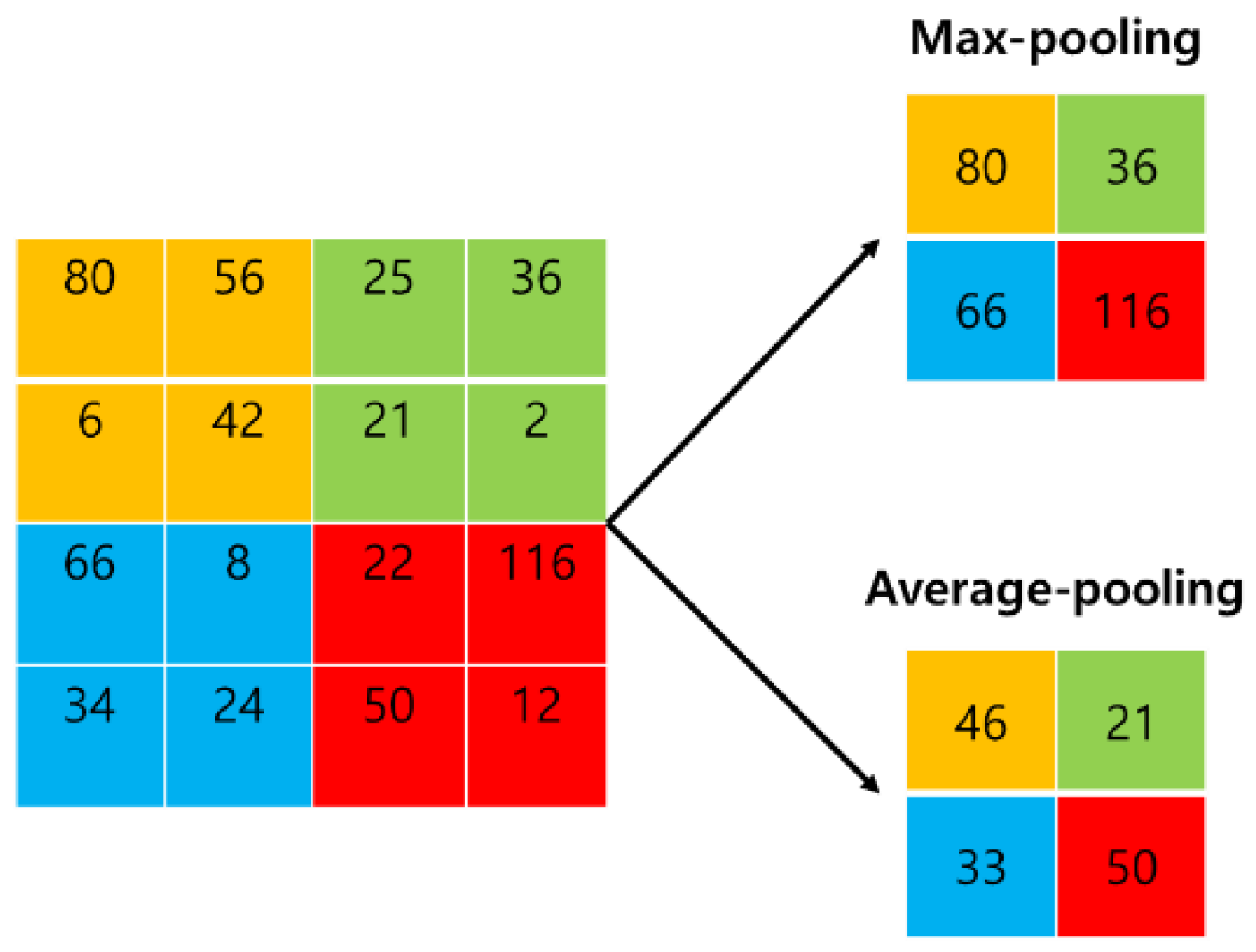
- Pooling layer
- Fully connected layer
- Output layer
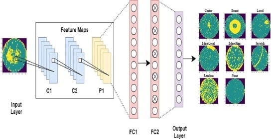
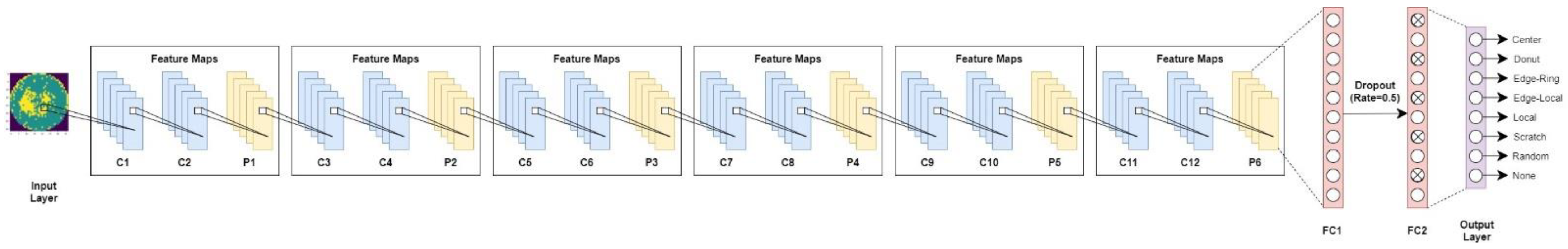
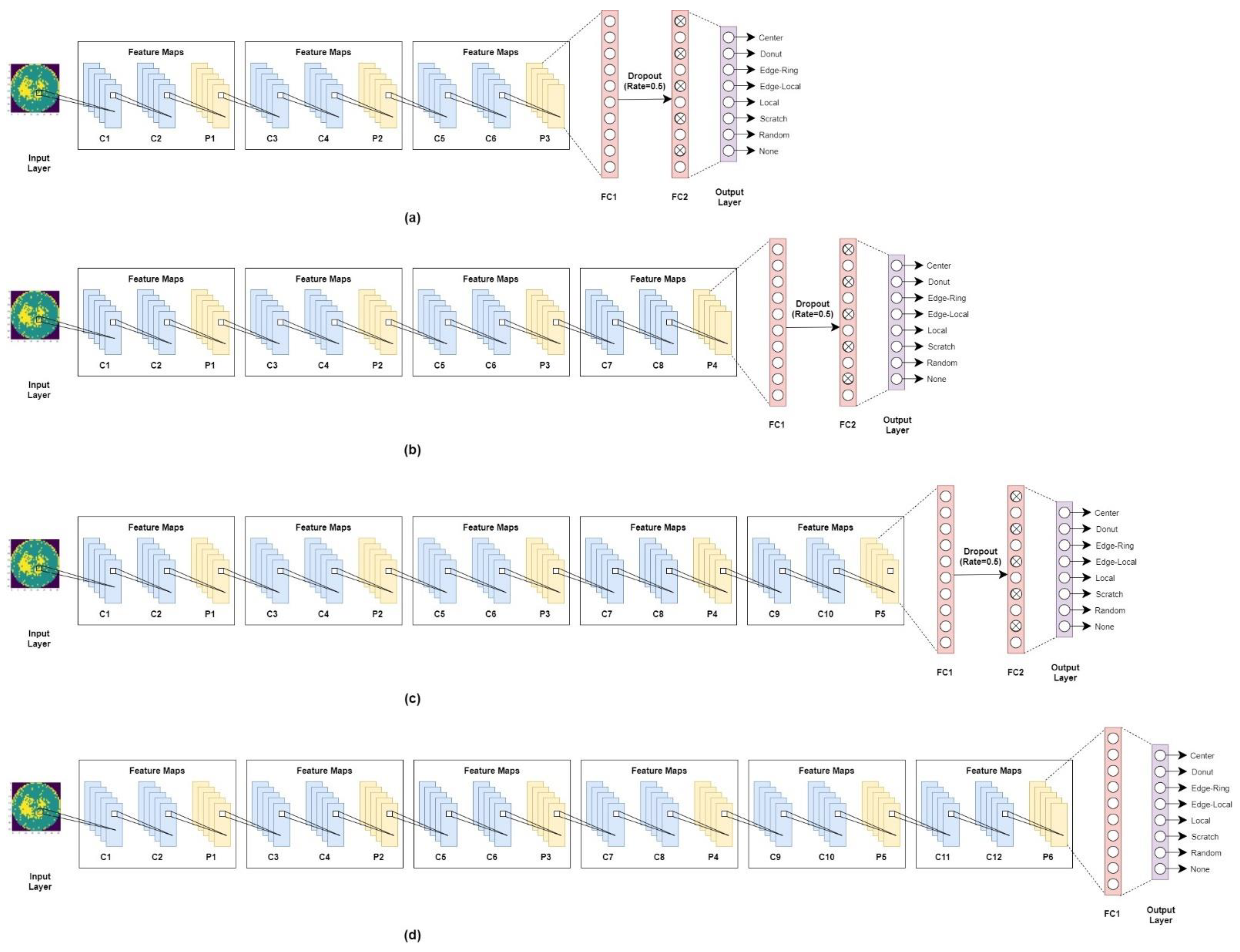
3.2. Proposed Method Architecture
3.3. Applied Machine Learning and Deep Learning Methods for Comparison
4. Experiments and Discussion
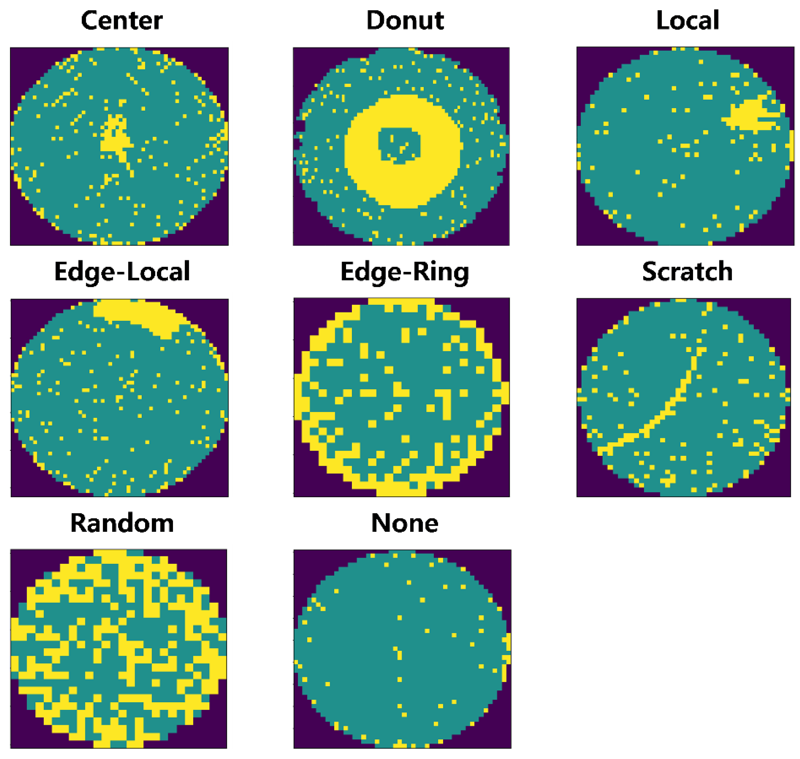
4.1. Data Description and Preprocessing
4.2. Performance Measures
4.3. Implementation Environment
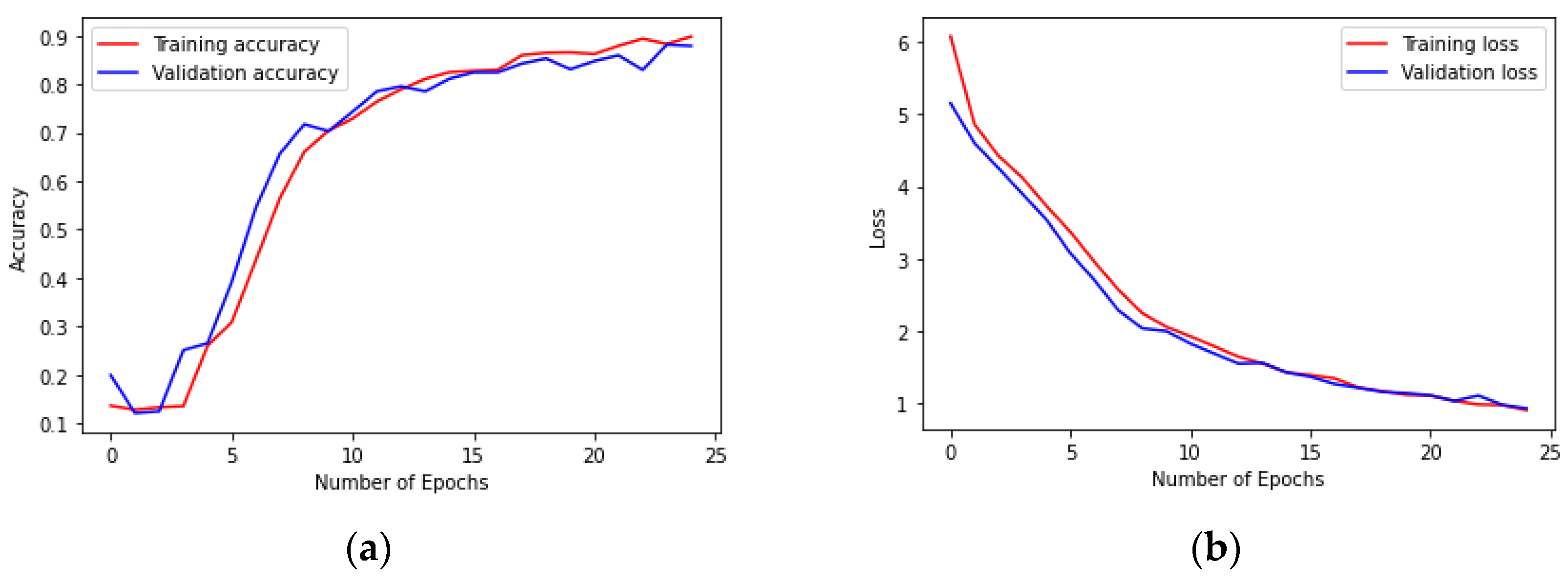
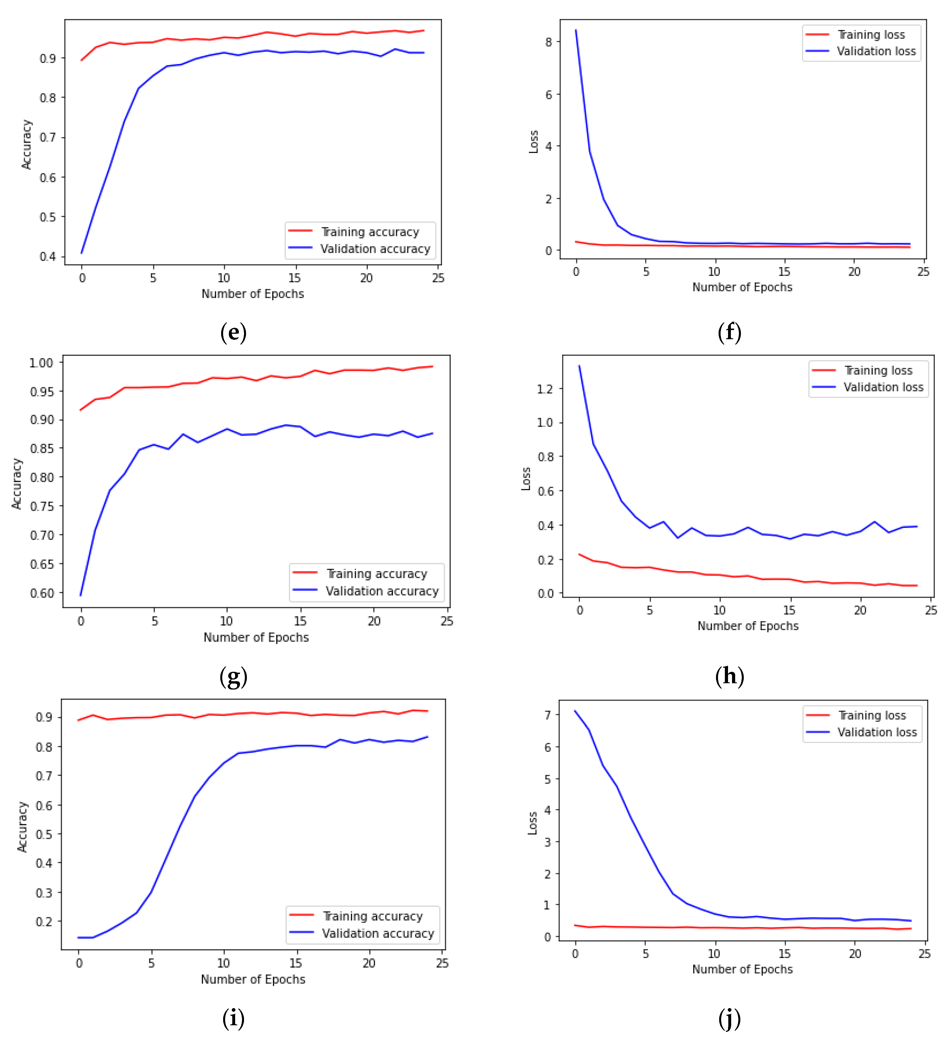
4.4. Results of Prediction Models and Discussion
5. Conclusions
Limitations
Author Contributions
Funding
Institutional Review Board Statement
Informed Consent Statement
Data Availability Statement
Conflicts of Interest
References
- Wang, R.; Chen, N. Defect pattern recognition on wafers using convolutional neural networks. Qual. Reliab. Eng. Int. 2020, 36, 1245–1257. [Google Scholar] [CrossRef]
- Yuan, T.; Kuo, W.; Bae, S.J. Detection of spatial defect patterns generated in semiconductor fabrication processes. IEEE Trans. Semicond. Manuf. 2011, 24, 392–403. [Google Scholar] [CrossRef]
- Wu, M.J.; Jang, J.S.R.; Chen, J.L. Wafer map failure pattern recognition and similarity ranking for large-scale data sets. IEEE Trans. Semicond. Manuf. 2014, 28, 1–12. [Google Scholar] [CrossRef]
- Piao, M.; Jin, C.H.; Lee, J.Y.; Byun, J.Y. Decision tree ensemble-based wafer map failure pattern recognition based on radon transform-based features. IEEE Trans. Semicond. Manuf. 2018, 31, 250–257. [Google Scholar] [CrossRef]
- Jin, C.H.; Na, H.J.; Piao, M.; Pok, G.; Ryu, K.H. A novel DBSCAN-based defect pattern detection and classification framework for wafer bin map. IEEE Trans. Semicond. Manuf. 2019, 32, 286–292. [Google Scholar] [CrossRef]
- Drozda-Freeman, A.; McIntyre, M.; Retersdorf, M.; Wooten, C.; Song, X.; Hesse, A. The application and use of an automated spatial pattern recognition (SPR) system in the identification and solving of yield issues in semiconductor manufacturing. In Proceedings of the 2007 IEEE/SEMI Advanced Semiconductor Manufacturing Conference, Stresa, Italy, 11–12 June 2007; pp. 302–305. [Google Scholar] [CrossRef]
- He, Q.P.; Wang, J. Fault detection using the k-nearest neighbor rule for semiconductor manufacturing processes. IEEE Trans. Semicond. Manuf. 2007, 20, 345–354. [Google Scholar] [CrossRef]
- Saqlain, M.; Jargalsaikhan, B.; Lee, J.Y. A voting ensemble classifier for wafer map defect patterns identification in semiconductor manufacturing. IEEE Trans. Semicond. Manuf. 2019, 32, 171–182. [Google Scholar] [CrossRef]
- Saqlain, M.; Abbas, Q.; Lee, J.Y. A deep convolutional neural network for wafer defect identification on an imbalanced dataset in semiconductor manufacturing processes. IEEE Trans. Semicond. Manuf. 2020, 33, 436–444. [Google Scholar] [CrossRef]
- Hsu, S.C.; Chien, C.F. Hybrid data mining approach for pattern extraction from wafer bin map to improve yield in semiconductor manufacturing. Int. J. Prod. Econ. 2007, 107, 88–103. [Google Scholar] [CrossRef]
- Choi, G.; Kim, S.H.; Ha, C.; Bae, S.J. Multi-step ART1 algorithm for recognition of defect patterns on semiconductor wafers. Int. J. Prod. Res. 2012, 50, 3274–3287. [Google Scholar] [CrossRef]
- Rawat, W.; Wang, Z. Deep convolutional neural networks for image classification: A comprehensive review. Neural Comput. 2017, 29, 2352–2449. [Google Scholar] [CrossRef]
- Li, Z.; Liu, F.; Yang, W.; Peng, S.; Zhou, J. A survey of convolutional neural networks: Analysis, applications, and prospects. IEEE Trans. Neural Netw. Learn. Syst. 2021, 1–21. [Google Scholar] [CrossRef]
- Ullah, I.; Manzo, M.; Shah, M.; Madden, M. Graph Convolutional Networks: Analysis, improvements and results. arXiv 2019, arXiv:1912.09592. [Google Scholar]
- Dimitriou, N.; Leontaris, L.; Vafeiadis, T.; Ioannidis, D.; Wotherspoon, T.; Tinker, G.; Tzovaras, D. Fault diagnosis in microelectronics attachment via deep learning analysis of 3-D laser scans. IEEE Trans. Ind. Electron. 2019, 67, 5748–5757. [Google Scholar] [CrossRef] [Green Version]
- Dimitriou, N.; Leontaris, L.; Vafeiadis, T.; Ioannidis, D.; Wotherspoon, T.; Tinker, G.; Tzovaras, D. A deep learning framework for simulation and defect prediction applied in microelectronics. Simul. Model. Pract. Theory 2020, 100, 102063. [Google Scholar] [CrossRef] [Green Version]
- Nakazawa, T.; Kulkarni, D.V. Wafer map defect pattern classification and image retrieval using convolutional neural network. IEEE Trans. Semicond. Manuf. 2018, 31, 309–314. [Google Scholar] [CrossRef]
- Shon, H.S.; Batbaatar, E.; Cho, W.S.; Choi, S.G. Unsupervised Pre-Training of Imbalanced Data for Identification of Wafer Map Defect Patterns. IEEE Access 2021, 9, 52352–52363. [Google Scholar] [CrossRef]
- Bagley, S.C.; White, H.; Golomb, B.A. Logistic regression in the medical literature: Standards for use and reporting, with particular attention to one medical domain. J. Clin. Epidemiol. 2001, 54, 979–985. [Google Scholar] [CrossRef]
- Breiman, L. Random forests. Mach. Learn. 2001, 45, 5–32. [Google Scholar] [CrossRef] [Green Version]
- Friedman, J.H. Greedy boosting approximation: A gradient boosting machine. Ann. Stat. 2001, 29, 1189–1232. [Google Scholar] [CrossRef]
- Simonyan, K.; Zisserman, A. Very deep convolutional networks for large-scale image recognition. arXiv 2014, arXiv:1409.1556. [Google Scholar]
- He, K.; Zhang, X.; Ren, S.; Sun, J. Deep residual learning for image recognition. In Proceedings of the IEEE Conference on Computer Vision and Pattern Recognition, Las Vegas, NV, USA, 27–30 June 2016; pp. 770–778. [Google Scholar] [CrossRef] [Green Version]
- Tan, M.; Le, Q. Efficientnet: Rethinking model scaling for convolutional neural networks. In Proceedings of the 36th International Conference on Machine Learning, Long Beach, CA, USA, 9–15 June 2019; PMLR 97. pp. 6105–6114. [Google Scholar]
- Mirlab.org. MIR Corpora. Available online: http://mirlab.org/dataSet/public/ (accessed on 6 October 2021).
- He, Q.P.; Wang, J. Principal component based k-nearest-neighbor rule for semiconductor process fault detection. In Proceedings of the 2008 American Control Conference, Seattle, WA, USA, 11–13 June 2008; pp. 1606–1611. [Google Scholar] [CrossRef]
- Chao, L.C.; Tong, L.I. Wafer defect pattern recognition by multi-class support vector machines by using a novel defect cluster index. Expert Syst. Appl. 2009, 36, 10158–10167. [Google Scholar] [CrossRef]
- Kang, S.; Cho, S.; An, D.; Rim, J. Using wafer map features to better predict die-level failures in final test. IEEE Trans. Semicond. Manuf. 2015, 28, 431–437. [Google Scholar] [CrossRef]
- Kim, D.; Kang, P.; Cho, S.; Lee, H.J.; Doh, S. Machine learning-based novelty detection for faulty wafer detection in semiconductor manufacturing. Expert Syst. Appl. 2012, 39, 4075–4083. [Google Scholar] [CrossRef]
- Jizat, J.A.M.; Majeed, A.P.A.; Nasir, A.F.A.; Taha, Z.; Yuen, E. Evaluation of the machine learning classifier in wafer defects classification. ICT Express 2021, 1–5. [Google Scholar] [CrossRef]
- Cheon, S.; Lee, H.; Kim, C.O.; Lee, S.H. Convolutional neural network for wafer surface defect classification and the detection of unknown defect class. IEEE Trans. Semicond. Manuf. 2019, 32, 163–170. [Google Scholar] [CrossRef]
- Kim, J.; Kim, H.; Park, J.; Mo, K.; Kang, P. Bin2Vec: A better wafer bin map coloring scheme for comprehensible visualization and effective bad wafer classification. Appl. Sci. 2019, 9, 597. [Google Scholar] [CrossRef] [Green Version]
- Nakazawa, T.; Kulkarni, D.V. Anomaly detection and segmentation for wafer defect patterns using deep convolutional encoder–decoder neural network architectures in semiconductor manufacturing. IEEE Trans. Semicond. Manuf. 2019, 32, 250–256. [Google Scholar] [CrossRef]
- Alawieh, M.B.; Boning, D.; Pan, D.Z. Wafer map defect patterns classification using deep selective learning. In Proceedings of the 2020 57th ACM/IEEE Design Automation Conference (DAC), San Francisco, CA, USA, 20–24 July 2020; pp. 1–6. [Google Scholar] [CrossRef]
- LeCun, Y.; Boser, B.; Denker, J.S.; Henderson, D.; Howard, R.E.; Hubbard, W.; Jackel, L.D. Backpropagation applied to handwritten zip code recognition. Neural Comput. 1989, 1, 541–551. [Google Scholar] [CrossRef]
- Chen, X.; Chai, Q.; Lin, N.; Li, X.; Wang, W. 1D convolutional neural network for the discrimination of aristolochic acids and their analogues based on near-infrared spectroscopy. Anal. Methods 2019, 11, 5118–5125. [Google Scholar] [CrossRef]
- Nair, V.; Hinton, G.E. Rectified linear units improve restricted boltzmann machines. In Proceedings of the 27th International Conference on International Conference on Machine Learning, Haifa, Israel, 21–24 June 2010; pp. 807–814. [Google Scholar]
- Sharma, S.; Sharma, S. Activation functions in neural networks. Towards Data Sci. 2017, 6, 310–316. [Google Scholar]
- He, K.; Zhang, X.; Ren, S.; Sun, J. Delving deep into rectifiers: Surpassing human-level performance on imagenet classification. In Proceedings of the IEEE international conference on computer vision, Santiago, Chile, 7–13 December 2015; pp. 1026–1034. [Google Scholar] [CrossRef] [Green Version]
- Yam, J.Y.; Chow, T.W. A weight initialization method for improving training speed in feedforward neural network. Neurocomputing 2000, 30, 219–232. [Google Scholar] [CrossRef]
- Bilgic, B.; Chatnuntawech, I.; Fan, A.P.; Setsompop, K.; Cauley, S.F.; Wald, L.L.; Adalsteinsson, E. Fast image reconstruction with L2--regularization. J. Magn. Reson. Imaging 2014, 40, 181–191. [Google Scholar] [CrossRef] [Green Version]
- Albawi, S.; Mohammed, T.A.; Al-Zawi, S. Understanding of a convolutional neural network. In Proceedings of the 2017 International Conference on Engineering and Technology (ICET), Antalya, Turkey, 21–23 August 2017; IEEE: Piscataway, NJ, USA; pp. 1–6. [Google Scholar]
- Srivastava, N.; Hinton, G.; Krizhevsky, A.; Sutskever, I.; Salakhutdinov, R. Dropout: A simple way to prevent neural networks from overfitting. J. Mach. Learn. Res. 2014, 15, 1929–1958. [Google Scholar]
- Kingma, D.P.; Ba, J. Adam: A method for stochastic optimization. arXiv 2014, arXiv:1412.6980. [Google Scholar]
- Abadi, M.; Agarwal, A.; Barham, P.; Brevdo, E.; Chen, Z.; Citro, C.; Corrado, G.S.; Davis, A.; Dean, J.; Devin, M.; et al. Tensorflow: Large-scale machine learning on heterogeneous distributed systems. arXiv 2016, arXiv:1603.04467. [Google Scholar]
- Keras.io. Keras Documentation. Available online: https://keras.io/ (accessed on 6 October 2021).
- Pedregosa, F.; Varoquaux, G.; Gramfort, A.; Michel, V.; Thirion, B.; Grisel, O.; Blondel, M.; Prettenhofer, P.; Weiss, R.; Dubourg, V.; et al. Scikit-learn: Machine learning in Python. J. Mach. Learn. Res. 2011, 12, 2825–2830. [Google Scholar]
- Jupyter.org. Project Jupyter. Available online: http://jupyter.org/ (accessed on 6 October 2021).
- Van Rossum, G.; Drake, F.L. Python 3 Reference Manual; CreateSpace: Scotts Valley, CA, USA, 2009. [Google Scholar]
- Pellicano, D.; Palamara, I.; Cacciola, M.; Calcagno, S.; Versaci, M.; Morabito, F.C. Fuzzy similarity measures for detection and classification of defects in CFRP. IEEE Trans. Ultrason. Ferroelectr. Freq. Control 2013, 60, 1917–1927. [Google Scholar] [CrossRef] [PubMed]
- Bardamova, M.; Konev, A.; Hodashinsky, I.; Shelupanov, A. A fuzzy classifier with feature selection based on the gravitational search algorithm. Symmetry 2018, 10, 609. [Google Scholar] [CrossRef] [Green Version]


| Layer | Detailed Parameters |
|---|---|
| Input layer | Size (224 × 224) |
| C1 | 16 3 × 3 2D convolutional layer (Relu) |
| C2 | 16 3 × 3 2D convolutional layer (Relu) |
| P1 | Max pooling layer 2 × 2 |
| C3 | 32 3 × 3 2D convolutional layer (Relu) |
| C4 | 32 3 × 3 2D convolutional layer (Relu) |
| P2 | Max pooling layer 2 × 2 |
| C5 | 64 3 × 3 2D convolutional layer (Relu) |
| C6 | 64 3 × 3 2D convolutional layer (Relu) |
| P3 | Max pooling layer 2 × 2 |
| C7 | 128 3 × 3 2D convolutional layer (Relu) |
| C8 | 128 3 × 3 2D convolutional layer (Relu) |
| P4 | Max pooling layer 2 × 2 |
| C9 | 256 3 × 3 2D convolutional layer (Relu) |
| C10 | 256 3 × 3 2D convolutional layer (Relu) |
| P5 | Max pooling layer 2 × 2 |
| C11 | 512 3 × 3 2D convolutional layer (Relu) |
| C12 | 512 3 × 3 2D convolutional layer (Relu) |
| P6 | Max pooling layer 2 × 2 |
| Flatten | |
| FC1 | Fully connected layer 512 (Relu) |
| Dropout layer | Dropout (rate = 0.5) |
| FC2 | Fully connected layer 512 (Relu) |
| Output layer | Output layer 8 (Softmax) |
| Type | Count |
|---|---|
| Center | 4296 (2.5%) |
| Donut | 555 (0.3%) |
| Local | 3597 (2.1%) |
| Edge-Local | 5199 (3.0%) |
| Edge-Ring | 9682 (5.6%) |
| Scratch | 1194 (0.7%) |
| Random | 866 (0.5%) |
| Near-Full | 149 (0.1%) |
| None | 147,431 (85.2%) |
| Total | 172,950 (100%) |
| Method | Classifier | Measure | Center | Donut | Edge-Ring | Edge-Local | Local | Random | Scratch | None | Average |
|---|---|---|---|---|---|---|---|---|---|---|---|
| ML-based Methods | LR | Precision | 0.9573 | 0.9024 | 0.7603 | 0.9899 | 0.7228 | 0.9783 | 0.9326 | 0.7879 | 0.8726 |
| Recall | 0.9106 | 0.8605 | 0.8214 | 0.9703 | 0.7019 | 1 | 0.9121 | 0.8387 | 0.8747 | ||
| F1-score | 0.9333 | 0.881 | 0.7897 | 0.98 | 0.7122 | 0.989 | 0.9222 | 0.8125 | 0.8729 | ||
| AUC | 0.9971 | 0.9862 | 0.9714 | 0.9992 | 0.9612 | 0.9993 | 0.9967 | 0.9772 | 0.9872 | ||
| RF | Precision | 0.9512 | 0.9012 | 0.7759 | 0.9706 | 0.7037 | 0.9783 | 0.9639 | 0.9316 | 0.9414 | |
| Recall | 0.9512 | 0.8488 | 0.8036 | 0.9802 | 0.7308 | 1 | 0.8791 | 0.8495 | 0.9004 | ||
| F1-score | 0.9512 | 0.8743 | 0.7895 | 0.9754 | 0.717 | 0.989 | 0.9195 | 0.8404 | 0.8958 | ||
| AUC | 0.9983 | 0.9871 | 0.9765 | 0.9997 | 0.9523 | 0.9999 | 0.9974 | 0.9846 | 0.9915 | ||
| GBDT | Precision | 0.9664 | 0.8889 | 0.7982 | 0.98 | 0.7054 | 0.989 | 0.9625 | 0.7961 | 0.8813 | |
| Recall | 0.935 | 0.8372 | 0.8125 | 0.9703 | 0.7596 | 1 | 0.8462 | 0.8817 | 0.9084 | ||
| F1-score | 0.9504 | 0.8623 | 0.8053 | 0.9751 | 0.7315 | 0.9945 | 0.9006 | 0.8367 | 0.8936 | ||
| AUC | 0.9988 | 0.9774 | 0.9752 | 0.9997 | 0.9686 | 0.9999 | 0.9969 | 0.987 | 0.9929 | ||
| DL-based Methods | VGG16 | Precision | 0.9508 | 0.9524 | 0.9706 | 0.8286 | 0.699 | 0.9556 | 0.7864 | 0.978 | 0.9644 |
| Recall | 0.9431 | 0.9302 | 0.9802 | 0.7768 | 0.6923 | 0.9451 | 0.871 | 0.9889 | 0.966 | ||
| F1-score | 0.9469 | 0.9412 | 0.9754 | 0.8018 | 0.6957 | 0.9503 | 0.8265 | 0.9834 | 0.9652 | ||
| AUC | 0.9982 | 0.9984 | 0.9996 | 0.9809 | 0.9651 | 0.9959 | 0.9881 | 0.9999 | 0.999 | ||
| VGG19 | Precision | 0.8897 | 0.9452 | 0.9524 | 0.9111 | 0.7297 | 0.9767 | 0.8073 | 1 | 0.9449 | |
| Recall | 0.9837 | 0.8023 | 0.9901 | 0.7321 | 0.7788 | 0.9231 | 0.9462 | 1 | 0.9919 | ||
| F1-score | 0.9344 | 0.8679 | 0.9709 | 0.8119 | 0.7535 | 0.9492 | 0.8713 | 1 | 0.9672 | ||
| AUC | 0.9979 | 0.9953 | 0.9994 | 0.9765 | 0.9585 | 0.9979 | 0.9928 | 1 | 0.999 | ||
| ResNet50 | Precision | 0.9652 | 0.9625 | 0.9899 | 0.8839 | 0.7154 | 0.9885 | 0.8723 | 1 | 0.9826 | |
| Recall | 0.9024 | 0.8953 | 0.9703 | 0.8839 | 0.8462 | 0.9541 | 0.8817 | 1 | 0.9512 | ||
| F1-score | 0.9328 | 0.9277 | 0.98 | 0.8839 | 0.7753 | 0.9663 | 0.877 | 1 | 0.9664 | ||
| AUC | 0.9973 | 0.9973 | 0.9999 | 0.9903 | 0.9677 | 0.9997 | 0.9928 | 1 | 0.9987 | ||
| ResNet101 | Precision | 0.9062 | 0.837 | 0.9709 | 0.7222 | 0.7439 | 0.957 | 0.8471 | 0.989 | 0.9476 | |
| Recall | 0.9431 | 0.8953 | 0.9901 | 0.8125 | 0.5865 | 0.978 | 0.7742 | 1 | 0.9716 | ||
| F1-score | 0.9243 | 0.8652 | 0.9804 | 0.7647 | 0.6559 | 0.9674 | 0.809 | 0.9945 | 0.9594 | ||
| AUC | 0.9937 | 0.992 | 0.9979 | 0.976 | 0.9563 | 0.9995 | 0.9846 | 1 | 0.9969 | ||
| EfficientNetB0 | Precision | 0.8333 | 0.7778 | 0.97 | 0.8037 | 0.625 | 0.9868 | 0.7865 | 0.9783 | 0.9058 | |
| Recall | 0.8537 | 0.814 | 0.9604 | 0.7679 | 0.7212 | 0.8242 | 0.7527 | 1 | 0.9269 | ||
| F1-score | 0.8434 | 0.7955 | 0.9652 | 0.7854 | 0.6696 | 0.8982 | 0.7692 | 0.989 | 0.9162 | ||
| AUC | 0.9744 | 0.9792 | 0.9987 | 0.9805 | 0.9508 | 0.9979 | 0.9717 | 1 | 0.9872 | ||
| Proposed DCNN | Precision | 0.9453 | 0.9419 | 0.9804 | 0.9052 | 0.8511 | 0.9888 | 0.914 | 0.9783 | 0.9618 | |
| Recall | 0.9837 | 0.9419 | 0.9901 | 0.9375 | 0.7692 | 0.967 | 0.914 | 1 | 0.9919 | ||
| F1-score | 0.9641 | 0.9419 | 0.9852 | 0.9211 | 0.8081 | 0.9778 | 0.914 | 0.989 | 0.9766 | ||
| AUC | 0.9979 | 0.998 | 0.9983 | 0.9853 | 0.9726 | 0.9996 | 0.9936 | 1 | 0.999 |
| Classifier | Precision | Recall | F1-score | AUC | Accuracy |
|---|---|---|---|---|---|
| LR | 0.8789 | 0.8769 | 0.8775 | 0.9906 | 0.875 |
| RF | 0.8845 | 0.8804 | 0.882 | 0.991 | 0.88 |
| GBDT | 0.8858 | 0.8803 | 0.882 | 0.9914 | 0.88 |
| VGG16 | 0.8902 | 0.8909 | 0.8902 | 0.991 | 0.8875 |
| VGG19 | 0.9015 | 0.8946 | 0.8949 | 0.9897 | 0.8938 |
| ResNet50 | 0.9222 | 0.9156 | 0.9179 | 0.9933 | 0.9137 |
| ResNet101 | 0.8717 | 0.8725 | 0.8702 | 0.9879 | 0.87 |
| EfficientNetB0 | 0.8452 | 0.8367 | 0.8394 | 0.9822 | 0.835 |
| Proposed DCNN | 0.9381 | 0.9379 | 0.9376 | 0.9933 | 0.9375 |
| Classifier | Precision | Recall | F1-score | AUC | Accuracy |
|---|---|---|---|---|---|
| DCNN1 | 0.9032 | 0.8903 | 0.8942 | 0.9912 | 0.8925 |
| DCNN2 | 0.9104 | 0.9127 | 0.9113 | 0.9908 | 0.91 |
| DCNN3 | 0.9037 | 0.9023 | 0.9006 | 0.9901 | 0.9012 |
| DCNN4 | 0.8673 | 0.8746 | 0.867 | 0.9867 | 0.8688 |
| Proposed DCNN | 0.9381 | 0.9379 | 0.9376 | 0.9933 | 0.9375 |
Publisher’s Note: MDPI stays neutral with regard to jurisdictional claims in published maps and institutional affiliations. |
© 2021 by the authors. Licensee MDPI, Basel, Switzerland. This article is an open access article distributed under the terms and conditions of the Creative Commons Attribution (CC BY) license (https://creativecommons.org/licenses/by/4.0/).
Share and Cite
Zheng, H.; Sherazi, S.W.A.; Son, S.H.; Lee, J.Y. A Deep Convolutional Neural Network-Based Multi-Class Image Classification for Automatic Wafer Map Failure Recognition in Semiconductor Manufacturing. Appl. Sci. 2021, 11, 9769. https://doi.org/10.3390/app11209769
Zheng H, Sherazi SWA, Son SH, Lee JY. A Deep Convolutional Neural Network-Based Multi-Class Image Classification for Automatic Wafer Map Failure Recognition in Semiconductor Manufacturing. Applied Sciences. 2021; 11(20):9769. https://doi.org/10.3390/app11209769
Chicago/Turabian StyleZheng, Huilin, Syed Waseem Abbas Sherazi, Sang Hyeok Son, and Jong Yun Lee. 2021. "A Deep Convolutional Neural Network-Based Multi-Class Image Classification for Automatic Wafer Map Failure Recognition in Semiconductor Manufacturing" Applied Sciences 11, no. 20: 9769. https://doi.org/10.3390/app11209769