Performance Analysis of RIS-Assisted FSO Communications over Fisher–Snedecor $\mathcal{F}$ Turbulence Channels

Abstract

The Fisher–Snedecor (F-S) $\mathcal{F}$ distribution has recently been introduced as a tractable turbulence-induced (TI) fading model that fits well with the experimental data. This paper provides a performance evaluation of a free-space optical (FSO) re-configurable intelligent surface (RIS)-assisted communications (ACs) link over the F-S $\mathcal{F}$ TI fading channels, assuming the intensity modulation–direct detection (IM–DD) technique. In particular, novel and closed-form (C-F) analytical expressions for the probability density function (PDF) and cumulative distribution function (CDF) of the end-to-end signal-to-noise ratio (SNR) in terms of Gaussian hyper-geometric functions are efficiently derived. Capitalizing on the obtained results, novel C-F analytical expressions for the moment generating function (${\mathcal{M}}_{MGF}$), outage probability (OP), average bit error rate (BER) and ergodic channel capacity $(C_{\gamma })$ of the FSO RIS-ACs system over the F-S $\mathcal{F}$ TI fading channels are provided and numerically evaluated under the various TI fading severity conditions. Furthermore, the second-order (S-O) statistical expressions for the level crossing rate (LCR) and average fade duration (AFD) are obtained and thoroughly examined for various FSO RIS-ACs system model parameters.

1. Introduction

Re-configurable intelligent surface (RIS)-assisted communications (ACs) are envisioned for beyond 5G and 6G wireless systems [1,2]. In a smart propagation environment, RIS blocks are capable of optimizing and improving system performances by controlling incident transmission waves in a directed and programmable way.

RIS-ACs for smart radio environments with suitable RIS applications are considered in [3]. Path-loss models for RIS-ACs supported by experimental and simulation results are provided in [4]. Moreover, a comparison between relay-ACs and RIS-ACs is provided in [5]. In [6], mmWave RIS-ACs systems are considered, whereas visible light communication (VLC) RIS-ACs systems are considered in [7,8].

Free-space optical (FSO) communication is a technology that, due to narrow beam widths, can be distinguished as highly secure, interference immune and energy efficient. Additionally, the FSO system is capable of providing a relatively large bandwidth and can be further distinguished as a license-free and cost effective transmission technology. In turn, the main cause of terrestrial FSO system performance degradation is atmospheric turbulence. The gamma–gamma (G-G) distribution is the most commonly used turbulence-induced (TI) fading model that is mathematically tractable and experimentally validated for moderate-to-strong TI fading conditions [9,10]. Moreover, the log-normal TI fading model is suitable for weak TI fading conditions, but is mathematically less tractable and often can lead to complex analytical expressions [11], whereas the general Malaga $\mathcal{M}$ TI fading model can be used to address weak-to-strong TI fading severity conditions, but is mathematically less tractable if compared with the G-G TI fading model [12].

The Fisher–Snedecor (F-S) $\mathcal{F}$ distribution has recently been proposed as an accurate and experimentally verified FSO TI fading model [13]. The F-S $\mathcal{F}$ TI fading channel for FSO communications with pointing errors for weak, moderate and strong TI fading conditions is addressed in [14], whereas the hybrid mmWave/FSO transmission over F-S $\mathcal{F}$ TI fading channels is considered in [15]. Moreover, the secrecy performance of the FSO system over F-S $\mathcal{F}$ TI fading propagation channels is reported in [16]. Initially, the F-S $\mathcal{F}$ distribution was proposed in [17], whereas, in [18,19,20,21], the authors considered wireless systems over the composite F-S $\mathcal{F}$ fading channels to account for multi-path and shadowing fading conditions. The second-order (S-O) statistics of composite $\mathcal{F}$ fading are given in [22], whereas the S-O metrics of bivariate F-S $\mathcal{F}$ distribution are considered in [23].

An FSO RIS-ACs system in moderate-to-strong severity conditions modelled over the G-G TI fading channels is well investigated in [24], whereas a mixed RF-FSO, RIS-ACs over G-G TI fading channels is further considered in [25]. Moreover, FSO RIS-ACs in weak-to-strong TI fading conditions modelled with both log-normal (in order to account for weak turbulence conditions) and G-G (in order to account for moderate-to-strong turbulence conditions) distributions are considered in [26]. A unified performance analysis of FSO RIS-ACs over G-G, F-S $\mathcal{F}$ and Malaga $\mathcal{M}$ TI fading channels for the first-order (F-O) statistical measures that are expressed through Meijer G and Fox H functions is conducted in [27]. In addition to F-O statistics, the S-O statistics can broaden the understanding of FSO RIS-ACs systems’ behaviour over rapidly time-variant TI fading channels. The S-O statistics for FSO systems over TI fading channels have been investigated in [28,29,30,31,32]. In [33], the authors analysed the S-O statistics of an FSO N-hop relay communications system over F-S $\mathcal{F}$ TI fading channels. Moreover, the S-O statistics have been considered in a variety of 5G and beyond 5G communication systems, [34,35,36,37]. The S-O performance measures such as the level crossing rate (LCR) and average fade duration (AFD) are of considerable importance for channel coding, the interleaver design, burst error (BE) rate and throughput analysis in FSO communications. Moreover, the BE rate can be used for the cross-layer design of error-control protocols with a rate adaptation in the FSO systems [38].

This paper provides a performance evaluation of an RIS-assisted FSO link over F-S $\mathcal{F}$ distribution evaluated for various TI fading conditions. Notice that the experimental concept of RIS is validated in [4] for distinct free-space path-loss models and the Fisher–Snedecor $\mathcal{F}$ distribution is considered in [13] for modelling the turbulence effects in FSO communications validating its use through Monte Carlo simulations. In this context, we provide novel, closed-form (C-F) PDF and CDF expressions in terms of the Gaussian hyper-geometric function. The C-F PDF and CDF expressions are further employed for the derivation of the moment generating function (${\mathcal{M}}_{MGF}$), OP, ergodic capacity ($C_{\gamma }$) and average BER for various binary modulation techniques. Moreover, the S-O statistical expressions are additionally provided and examined. The F-O and the S-O statistical results of the considered FSO RIS-ACs link exposed to various TI fading severity conditions are numerically evaluated and analysed. To the best of the author’s knowledge, there are no reported results on the unified F-O and S-O performance analysis of the FSO RIS-ACs over F-S $\mathcal{F}$ TI fading channels.

2. Fisher–Snedecor $\mathcal{F}$ Composite Fading Model

The Fisher–Snedecor (F-S) $\mathcal{F}$ turbulence-induced (TI) fading model attracts significant interest in the field of FSO communications [13,14,15,16,27,33]. The F-S $\mathcal{F}$ TI fading distribution can be expressed as the product of independent and identically distributed (i.i.d) Gamma (G) and normalized inverse Gamma (I-G) random variables (RVs) [13,33]:

$$Z_{\mathcal{F}S}=X_G{Y}_{IG}=X_G\frac{1}{Y_G}$$

(1)

where $X_G$ and $Y_{IG}$ are G and normalized I-G RVs, respectively. Since the normalized I-G RV can be mathematically expressed as $Y_{IG}=\frac{1}{Y_G}$, the probability density functions (PDFs) of $X_G$ and $Y_G$ are given as:

$$p_{X_G}(x_G)=\frac{{(m_{G_1}/{\Omega }_{G_1})}^{m_{G_1}}}{\Gamma (m_{G_1})}{(x_G)}^{m_{G_1}-1}{e}^{-\frac{m_{G_1}}{{\Omega }_{G_1}}(x_G)}$$

(2)

$$p_{Y_G}(y_G)=\frac{{\left((m_{G_2}-1)/{\Omega }_{G_2}\right)}^{m_{G_2}}}{\Gamma (m_{G_2})}{(y_G)}^{m_{G_2}-1}{e}^{-\frac{(m_{G_2}-1)}{{\Omega }_{G_2}}(y_G)}$$

(3)

whose shape parameters are $m_{G_1}$ and $m_{G_2}$, respectively, whereas the mean powers are ${\Omega }_{G_1}$ and ${\Omega }_{G_2}$, respectively. The $\Gamma (·)$ is the Gamma function ([39], Equation (8.310.1)). By applying a transformation of RVs, ${\gamma }_{x_G}={X_G}^2$ and ${\gamma }_{y_G}={Y_G}^2$, the PDFs of the squared G and the normalised squared I-G RVs are, respectively:

$$\begin{array}{c}\hfill p_{{\gamma }_{x_G}}({\gamma }_{x_G})=\left|\frac{d{x}_G}{d{\gamma }_{x_G}}\right|p_{X_G}({{\gamma }_{x_G}}^{1/2})=\frac{{(m_{G_1}/{\Omega }_{G_1})}^{m_{G_{}1}}}{2\Gamma (m_{G_1})}{({\gamma }_{x_G})}^{\frac{1}{2}{m}_{G_1}-1}{e}^{-\frac{m_{G_1}}{{\Omega }_{G_1}}{({\gamma }_{x_G})}^{\frac{1}{2}}}\end{array}$$

(4)

$$\begin{array}{c}\hfill p_{{\gamma }_{y_G}}({\gamma }_{y_G})=\left|\frac{d{y}_G}{d{\gamma }_{y_G}}\right|p_{Y_G}({{\gamma }_{y_G}}^{1/2})=\frac{{\left((m_{G_2}-1)/{\Omega }_{G_2}\right)}^{m_{G_2}}}{2\Gamma (m_{G_2})}{({\gamma }_{y_G})}^{\frac{1}{2}{m}_{G_2}-1}{e}^{-\frac{(m_{G_2}-1)}{{\Omega }_{G_2}}{({\gamma }_{y_G})}^{\frac{1}{2}}}\end{array}$$

(5)

The PDF of ${\gamma }_{\mathcal{F}S}=\frac{{\gamma }_{x_G}}{{\gamma }_{y_G}}$ can be obtained as:

$$p_{{\gamma }_{\mathcal{F}S}}(\gamma )={\int }_0^{\infty }\left|\frac{d{\gamma }_{x_G}}{d{\gamma }_{\mathcal{F}S}}\right|p_{{\gamma }_{x_G}}(\gamma \times {\gamma }_{y_G})p_{{\gamma }_{y_G}}({\gamma }_{y_G})d{\gamma }_{y_G}$$

(6)

where $\left|\frac{d{\gamma }_{x_G}}{d{\gamma }_{\mathcal{F}S}}\right|={\gamma }_{y_G}.$ From (4) to (6), and by applying ([39], Equation (3.326.2)) and ([39], Equation (8.384.1)), respectively, the PDF of ${\gamma }_{\mathcal{F}S}$ can be written as:

$$\begin{array}{ccc}\hfill p_{{\gamma }_{\mathcal{F}S}}(\gamma )& =& \frac{{(\frac{m_{G_1}}{{\Omega }_{G_1}})}^{m_{G_1}}{(\frac{m_{G_2}-1}{{\Omega }_{G_2}})}^{m_{G_2}}{({\Omega }_{G_2}{\Omega }_{G_1})}^{m_{G_1}+m_{G_2}}}{{({\Omega }_{G_2}{m}_{G_1}{\gamma }^{\frac{1}{2}}+{\Omega }_{G_1}(m_{G_2}-1))}^{m_{G_1}+m_{G_2}}}\frac{{\gamma }^{\frac{1}{2}{m}_{G_1}-1}}{2\beta (m_{G_1},m_{G_2})}\hfill \end{array}$$

(7)

where $\beta (·,·)$ is the Beta function ([39], Equation (8.380.1)). It can be concluded that $p_{{\gamma }_{\mathcal{F}S}}({\gamma }_{\mathcal{F}S})$ in (7) for ${\Omega }_{G_1}={\overline{\gamma }}^{1/2}$, ${\Omega }_{G_2}=1$, $m_{G_1}=a$ and $m_{G_2}=b$ reduces to the PDF of F-S $\mathcal{F}$ TI fading distribution given by ([13], Equation (20)).

3. FSO RIS-ACs Link over F-S $\mathcal{F}$ TI fading Channels

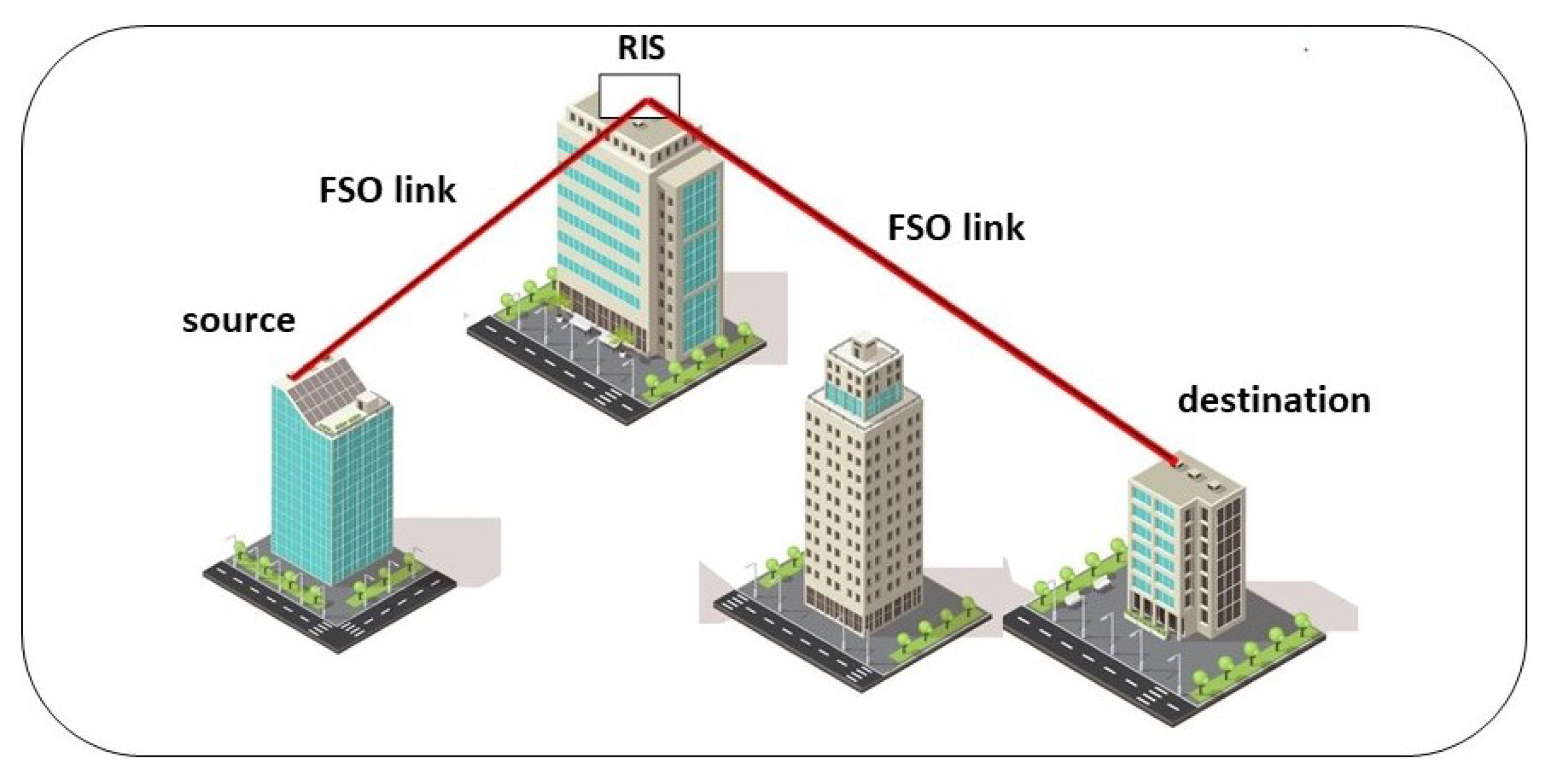
We considered an FSO RIS-ACs system over F-S $\mathcal{F}$ TI fading channels. A simplified block scheme is presented in Figure 1. It was assumed that the RIS module ideally reflects the FSO signal and that the system is not influenced by pointing errors. The output symbol at the receiver y can be expressed as [24]:

$$\begin{array}{c}\hfill y={E_s}^{1/2}x(h_1{\mu }_r{e}^{j{\theta }_r}{h}_2)+n\end{array}$$

(8)

where x is the transmitted symbol, $E_s$ is the symbol’s energy and n is AWGN. $h_1$ and $h_2$ are channel coefficients from source-to-RIS (S-RIS) and RIS-to-destination (RIS-D), respectively, whereas the quantity ${\mu }_r{e}^{j{\theta }_r}$ is deterministic in nature and describes the RIS part of the system under consideration. In detail, ${\mu }_r\in [0,1]$ is a coefficient of amplitude reflection and ${\theta }_r\in [0,2\pi ]$ is a phase [40].

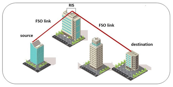
Figure 1. Simplified block scheme of FSO RIS-ACs link.

The PDF of the received signal-to-noise ratio (SNR) for the considered FSO RIS-ACs transmission link can be expressed as ([24], Equation (17)):

$$p_{\gamma }(\gamma )={\int }_0^{\infty }\frac{1}{r}{p}_{{\gamma }_{h_1}}(\frac{\gamma }{r})p_{{\gamma }_{h_2}}(r)dr$$

(9)

where $p_{{\gamma }_{h_1}}$ and $p_{{\gamma }_{h_2}}$ are SNR’s PDFs of the links $h_1$ and $h_2$, respectively, which in the case of intensity modulation–direct detection (IM–DD) with the on–off keying (OOK) technique for Fisher–Snedecor $\mathcal{F}$ TI fading distribution can be written as ([13], Equation (20)):

$$\begin{array}{ccc}\hfill p_{{\gamma }_{h_i}}({\gamma }_i)& =& \frac{{a_i}^{a_i}{(b_i-1)}^{b_i}{\overline{{\gamma }_i}}^{b_i/2}{\gamma }_i^{a_i/2-1}}{2\beta (a_i,b_i){(a_i{{\gamma }_i}^{1/2}+(b_i-1){\overline{{\gamma }_i}}^{1/2})}^{a_i+b_i}},i=1,2;\hfill \end{array}$$

(10)

where $\overline{{\gamma }_i}$ is the average SNR, whereas $a_i$ and $b_i$ are Fisher–Snedecor $\mathcal{F}$ small-scale and large-scale cells related to TI fading severity conditions, respectively. The scintillation indexes of S-RIS and RIS-D F-S $\mathcal{F}$ TI fading can be expressed as ([13], Equation (10)), respectively:

$$\begin{array}{ccc}& {\sigma }_{{\gamma }_{h_i}}^2& =\left(1+\frac{1}{a_i}\right)\left(1+\frac{1}{b_i-2}\right)-1,b_i>2;i=1,2;\hfill \end{array}$$

(11)

The $a_i$ and $b_i$ can be written as ([13], Equation (12a)) and ([13], Equation (12b)), respectively:

$$a_i=\frac{1}{e^{{\sigma }_{ln{I}_{a_i}}^2}-1},b_i=\frac{1}{e^{{\sigma }_{ln{I}_{b_i}}^2}-1}+2,i=1,2;$$

(12)

where ${\sigma }_{ln{I}_{a_i}}^2$ and ${\sigma }_{ln{I}_{b_i}}^2$ are normalized log-variances of $I_{a_i}$ and $I_{b_i}$, respectively. Moreover, $I_{a_i}$ and $I_{b_i}$ are Gamma ([13] and Inverse normalized Gamma ([13], Equation (4)) distributions, respectively. Under the assumption of spherical propagation, ${\sigma }_{ln{I}_{a_i}}^2$ is ([14], Equation (3)):

$${\sigma }_{ln{I}_{a,i}}^2=\frac{0.51{\sigma }_{SP,i}^2{(1+0.69{\sigma }_{SP,i}^{12/5})}^{-5/6}}{1+0.90d_i^2{({\sigma }_i/{\sigma }_{SP,i}^2)}^{12/5}+0.62d_i^2{\sigma }_i^{12/5}}$$

(13)

where ${\sigma }_{SP,i}$, $\mathit{i}=1,2$ is the spherical scintillation index (SSI) of S-RIS and RIS-D, respectively, and for weak fluctuation conditions, ${\sigma }_{SP,i}$ is:

$$\begin{array}{ccc}\hfill {\sigma }_{SP,i}^2& =& 9.65{\sigma }_i^2\left(0.4{(1+9/Q_{l_i}^2)}^{11/12}\left[sin(\frac{11}{6}arctan\frac{Q_{l_i}}{3})\right.\right.+\frac{2.61}{{(9+Q_{l_i}^2)}^{1/4}}sin(\frac{4}{3}arctan\frac{Q_{l_i}}{3})\hfill \\ & & -\left.\left.\frac{0.52}{{(9+Q_{l_i}^2)}^{7/24}}sin(\frac{5}{4}arctan\frac{Q_{l_i}}{3})\right]-3.5/Q_{l_i}^{\frac{5}{6}}\right)\hfill \end{array}$$

(14)

where $Q_{l_i}=10.89S_i/(B_i{l}_{0_i}^2)$, $S_i$ is the transmission distance, $B_i=2\pi /{\lambda }_i$ is the wave-number, ${\lambda }_i$ is the optical wavelength and $l_{0_i}$ is the inner-scale of the S-RIS and RIS-D Fisher–Snedecor $\mathcal{F}$ TI fading model. Furthermore, $d_i=\sqrt{B_i{D}_i^2/4S_i}$ and ${\sigma }_i^2=0.5C_{n_i}^2{B}_i^{7/6}{S}_i^{11/6}$, where ${\sigma }_i^2$ represents the Rytov variance. $D_i$ is the receiver aperture diameter and $C_{n_i}^2$ is the refractive index for i$=1,2$. The ${\sigma }_{ln{I}_{b,i}}^2$ can be written as ([14], Equation (5)):

$${\sigma }_{ln{I}_{b,i}}^2={\sigma }_{ln{I}_{b,i}}^2(l_{0_i})-{\sigma }_{ln{I}_{b,i}}^2(L_{0_i})$$

(15)

where ${\sigma }_{ln{I}_{b,i}}^2(l_{0_i})$ and ${\sigma }_{ln{I}_{b,i}}^2(L_{0_i})$ are the inner and outer large-scale log-irradiance variances, respectively, that can be expressed as:

$$\begin{array}{ccc}\hfill {\sigma }_{ln{I}_{b,i}}^2(u_i)& =& 0.04{\sigma }_i^2{\eta }_i(u_i)+Q_{l_i}{)}^{7/6}\hfill \\ & & \times [1+1.75{(\frac{{\eta }_i(u_i)}{{\eta }_i(u_i)+Q_{l_i}})}^{1/2}-{(\frac{{\eta }_i(u_i)}{{\eta }_i(u_i)+Q_{l_i}})}^{7/12}]\hfill \end{array}$$

(16)

where $u_i=\{l_{0_i},L_{0_i}\}$. Additionally, ${\eta }_i(l_{0_i})=\frac{8.56}{1+0.18d_i^2+0.20{\sigma }_i^2{Q}_{l_i}^{\frac{1}{6}}}$, ${\eta }_i(L_{0_i})=\frac{Q_{0_i}{\eta }_i(l_{0_i})}{Q_{0_i}+{\eta }_i(l_{0_i})}$ and $Q_{0_i}=\frac{64{\pi }^2{S}_i}{B_i{L}_{0_i}^2}$.

3.1. Probability Density Function ($p_{\gamma }$)

The probability density function ($p_{\gamma }$) of the considered FSO RIS-ACs system over F-S $\mathcal{F}$ TI fading channels, after substituting (10) in (9), can be written as:

$$\begin{array}{ccc}\hfill p_{\gamma }(\gamma )& =& \frac{{a_1}^{a_1}{(b_1-1)}^{b_1}{a_2}^{a_2}{(b_2-1)}^{b_2}{\overline{\gamma }}^{(b_1+b_2)/2}{\gamma }^{a_1/2-1}}{4\beta (a_1,b_1)\beta (a_2,b_2)}\hfill \\ & & \times {\int }_0^{\infty }\frac{r^{a_2/2-a_1/2-1}dr}{{(a_1{\gamma }^{1/2}{r}^{-1/2}+(b_1-1){\overline{\gamma }}^{1/2})}^{a_1+b_1}{(a_2{r}^{1/2}+(b_2-1){\overline{\gamma }}^{1/2})}^{a_2+b_2}}\hfill \end{array}$$

(17)

where $\overline{\gamma }=\overline{{\gamma }_1}=\overline{{\gamma }_2}$. Using ([39], Equation (3.259.3)) and some additional mathematical manipulations, the C-F expression for $p_{\gamma }(\gamma )$ of FSO RIS-ACs in terms of the Beta and Gaussian hyper-geometric function ${}_2{F}_1(·,·;·;·)$ ([39], Equation (9.10)) is derived as:

$$\begin{array}{ccc}\hfill p_{\gamma }(\gamma )& =& \frac{{a_1}^{a_2}{a_2}^{a_2}{\gamma }^{a_2/2-1}}{2\beta (a_1,b_1)\beta (a_2,b_2){(b_1-1)}^{a_2}{(b_2-1)}^{a_2}{\overline{\gamma }}^{a_2}}\beta (a_2+b_1,a_1+b_2)\hfill \\ & & \times {}_2{F}_1\left(a_2+b_2,a_2+b_1;a_1+b_1+a_2+b_2;1-\frac{a_1{a}_2{\gamma }^{1/2}}{(b_1-1)(b_2-1)\overline{\gamma }}\right)\hfill \end{array}$$

(18)

3.2. Cumulative Distribution Function ($F_{\gamma }$)

The cumulative distribution function ($F_{\gamma }$) of an FSO RIS-ACs system over the F-S $\mathcal{F}$ TI fading channels can be obtained by using the following formulae:

$$\begin{array}{c}\hfill F_{\gamma }(\gamma )={\int }_0^{\gamma }{p}_{\gamma }(\tau )d\tau \end{array}$$

(19)

After substituting (17) in (19), the $F_{\gamma }(\gamma )$ of an FSO RIS-ACs system can be written as:

$$\begin{array}{ccc}\hfill F_{\gamma }(\gamma )& =& \frac{{a_1}^{a_1}{(b_1-1)}^{b_1}{a_2}^{a_2}{(b_2-1)}^{b_2}{\overline{\gamma }}^{(b_1+b_2)/2}}{4\beta (a_1,b_1)\beta (a_2,b_2)}\hfill \\ & & \times {\int }_0^{\infty }\frac{r^{a_2/2+b_1/2-1}dr}{{(a_2{r}^{1/2}+(b_2-1){\overline{\gamma }}^{1/2})}^{a_2+b_2}}{H}_1\hfill \end{array}$$

(20)

where $H_1$ is:

$$\begin{array}{c}\hfill H_1={\int }_0^{\gamma }d\tau \frac{{\tau }^{a_1/2-1}}{{(a_1{\tau }^{1/2}+(b_1-1){\overline{\gamma }}^{1/2}{r}^{1/2})}^{a_1+b_1}}\end{array}$$

(21)

The integral form (I-F) expression $H_1$ can be solved using the variable substitution, $s=a_1{\tau }^{1/2}+(b_1-1){\overline{\gamma }}^{1/2}{r}^{1/2}$ and, then, by applying the binomial formula ([39], Equation (1.111)). The value of $H_1$ was calculated and given as:

$$\begin{array}{ccc}\hfill H_1& =& \frac{2}{{a_1}^{a_1}}\sum _{k=0}^{a_1-1}\left(\genfrac{}{}{0pt}{}{a_1-1}{k}\right){(-1)}^k\frac{{((b_1-1){\overline{\gamma }}^{1/2}{r}^{1/2})}^k}{b_1+k}\hfill \\ & & \times \left(\frac{1}{(b_1-1){\overline{\gamma }}^{1/2}{r}^{1/2}{)}^{b_1+k}}-\frac{1}{{(a_1{\gamma }^{1/2}+(b_1-1){\overline{\gamma }}^{1/2}{r}^{1/2})}^{b_1+k}}\right)\hfill \end{array}$$

(22)

After substituting (22) in (20) and, then, by using ([39], Equation (3.259.3)), the C-F $F_{\gamma }(\gamma )$ expression of the received SNR for the considered FSO RIS-ACs was calculated and given as:

$$\begin{array}{ccc}& & F_{\gamma }(\gamma )=\frac{{(b_1-1)}^{b_1}{a_2}^{a_2}{(b_2-1)}^{b_2}{\overline{\gamma }}^{(b_1+b_2)/2}}{\beta (a_1,b_1)\beta (a_2,b_2)}\sum _{k=0}^{a_1-1}\left(\genfrac{}{}{0pt}{}{a_1-1}{k}\right){(-1)}^k\frac{{((b_1-1){\overline{\gamma }}^{1/2})}^k}{b_1+k}\hfill \\ & & \times \left(\frac{{(\frac{(b_2-1){\overline{\gamma }}^{1/2}}{a_2})}^{a_2}\beta (a_2,b_2)}{{((b_1-1){\overline{\gamma }}^{1/2})}^{b_1+k}{((b_2-1){\overline{\gamma }}^{1/2})}^{a_2+b_2}}-\frac{{(\frac{a_1{\gamma }^{1/2}}{(b_1-1){\overline{\gamma }}^{1/2}})}^{a_2+b_1+k}\beta (a_2+b_1+k,b_2)}{{(a_1{\gamma }^{1/2})}^{b_1+k}(b_2-1){\overline{\gamma }}^{1/2}{)}^{a_2+b_2}}\right.\hfill \\ & & \times \left.{}_2{F}_1\left(a_2+b_2,a_2+b_1+k;b_1+a_2+b_2+k;1-\frac{a_1{a}_2{\gamma }^{1/2}}{(b_1-1)(b_2-1)\overline{\gamma }}\right)\right)\hfill \end{array}$$

(23)

3.3. Moment Generating Function (${\mathcal{M}}_{MGF}$)

The ${\mathcal{M}}_{MGF}$ of the end-to-end SNR for the considered FSO RIS-ACs system can be derived as ([24], Equation (28)):

$$\begin{array}{c}\hfill {\mathcal{M}}_{MGF}(s)=s{\int }_0^{\gamma }{e}^{-s\gamma }{F}_{\gamma }(\gamma )d\gamma \end{array}$$

(24)

The C-F ${\mathcal{M}}_{MGF}(s)$ was derived in terms of the Meijer G function ([41], Equation (07.34.02.0001.01)), using ([41], Equation (07.23.26.0007.01)) and ([41], Equation (07.34.21.0088.01)), respectively, and obtained as:

$$\begin{array}{ccc}& & {\mathcal{M}}_{MGF}(s)=\frac{{(b_1-1)}^{b_1}{a_2}^{a_2}{(b_2-1)}^{b_2}{\overline{\gamma }}^{(b_1+b_2)/2}}{\beta (a_1,b_1)\beta (a_2,b_2)}\sum _{k=0}^{a_1-1}\left(\genfrac{}{}{0pt}{}{a_1-1}{k}\right){(-1)}^k\frac{{((b_1-1){\overline{\gamma }}^{1/2})}^k}{b_1+k}\hfill \\ & & \times \left(\frac{{(\frac{(b_2-1){\overline{\gamma }}^{1/2}}{a_2})}^{a_2}\beta (a_2,b_2)}{{((b_1-1){\overline{\gamma }}^{1/2})}^{b_1+k}{((b_2-1){\overline{\gamma }}^{1/2})}^{a_2+b_2}}-\frac{{(\frac{a_1}{(b_1-1){\overline{\gamma }}^{1/2}})}^{a_2+b_1+k}\beta (a_2+b_1+k,b_2)s}{{(a_1)}^{b_1+k}(b_2-1){\overline{\gamma }}^{1/2}{)}^{a_2+b_2}}\right.\hfill \\ & & \times \frac{\Gamma (b_1+a_2+b_2+k)}{\Gamma (a_2+b_2)\Gamma (b_1+a_2+k)\Gamma (b_1+k)\Gamma (b_2)}\frac{2^{a_2+2b_2+k-1}}{{(2\pi )}^2{s}^{(1/2)a_2+1}}\hfill \\ & & \times \left.G_{5,4}^{4,5}\left(\frac{{(a_1{a}_2)}^2}{{(s(b_1-1)(b_2-1)\overline{\gamma })}^2}\left|\begin{array}{c}-\frac{1}{2}{a}_2,\frac{1-a_2-b_2}{2},\frac{2-a_2-b_2}{2},\frac{1-a_2-b_2-k}{2},\frac{2-a_2-b_2-k}{2}\\ 0,\frac{1}{2},-\frac{a_2}{2},\frac{1-a_2}{2}\end{array}\right.\right)\right)\hfill \end{array}$$

(25)

Remark 1.

To date, the statistical distribution functions of the FSO communications based on RIS subject to turbulence effects have been derived. In the context of 5G and 6G, FSO communications coexist with other radiofrequency (RF) systems, e.g., a point-to-point system transmitting in the mmWave frequency domain. Thus, it is possible to combine both frequency domains in order to generate a hybrid FSO and RF system. Although the evaluation of this hybrid system is out of the scope of this paper, it would improve the performance of any system operating independently and its evaluation will be considered in further works.

4. Performance Analysis of an FSO RIS-ACs Link over F-S $\mathcal{F}$ TI fading Channels

The first-order (F-O) performance metrics of the single-input single-output (SISO) FSO RIS-ACs link over F-S $\mathcal{F}$ TI fading channels based on end-to-end average SNR for IM–DD with the OOK technique are provided in the following Section.

4.1. Outage Probability ($P_{\gamma }$)

The OP $(P_{\gamma })$ for a given SNR threshold ${\gamma }_{th}$ of an FSO RIS-ACs over F-S $\mathcal{F}$ TI fading propagation channels for IM–DD with the OOK technique was calculated as:

$$P_{\gamma }({\gamma }_{th})=P_{\gamma }(\gamma \le {\gamma }_{th})=F_{\gamma }({\gamma }_{th})$$

(26)

where $F_{\gamma }$ was already derived in (23). It is important to note that $F_{\gamma }$ was valid only for the integer values of $a_1$, since $F_{\gamma }$ was derived as a finite series expression. The numerical analysis of the OP for an FSO RIS-ACs system over Fisher–Snedecor $\mathcal{F}$ TI fading channels was provided in the Numerical Results.

4.2. Average Bit Error Rate ($P_{BER}$)

The average bit error rate ($P_{BER}$) can be defined as the rate at which errors occur in the considered FSO RIS-ACs transmission system. The $P_{BER}$ of the received SNR for various binary modulation techniques of the FSO RIS-ACs system in F-S $\mathcal{F}$ TI fading propagation environment can be calculated using ([42], Equation (25)):

$$\begin{array}{c}\hfill P_{BER}(\gamma )=\frac{q^p}{2\Gamma (p)}{\int }_0^{\infty }{\gamma }^{p-1}{F}_{\gamma }(\gamma )e^{-q\gamma }d\gamma \end{array}$$

(27)

where p and q are the parameters of different modulation types. In particular, $P_{BER}(\gamma )$ for the non-coherent binary frequency shift keying (NBFSK) (p = 1, q = 1/2), binary frequency shift keying (BFSK) (p = 1/2, q = 1/2), binary phase shift keying (BPSK) (p = 1/2, q = 1) and differential binary phase shift keying (DBPSK) (p = 1, q = 1) can be obtained from (27). According to (23), $P_{BER}(\gamma )$ can be written as:

$$\begin{array}{ccc}\hfill P_{BER}(\gamma )& =& \frac{q^p}{2\Gamma (p)}\frac{{(b_1-1)}^{b_1}{a_2}^{a_2}{(b_2-1)}^{b_2}{\overline{\gamma }}^{(b_1+b_2)/2}}{\beta (a_1,b_1)\beta (a_2,b_2)}\sum _{k=0}^{a_1-1}\left(\genfrac{}{}{0pt}{}{a_1-1}{k}\right){(-1)}^k\frac{{((b_1-1){\overline{\gamma }}^{1/2})}^k}{b_1+k}\hfill \\ & & \times \left(\frac{{\left(\frac{1}{q}\right)}^p\Gamma (p){(\frac{(b_2-1){\overline{\gamma }}^{1/2}}{a_2})}^{a_2}\beta (a_2,b_2)}{{((b_1-1){\overline{\gamma }}^{1/2})}^{b_1+k}{((b_2-1){\overline{\gamma }}^{1/2})}^{a_2+b_2}}-H_2\right)\hfill \end{array}$$

(28)

where $H_2$ is given as:

$$\begin{array}{ccc}\hfill H_2& =& {\int }_0^{\infty }{\gamma }^{p-1}{e}^{-q\gamma }\frac{{(\frac{a_1{\gamma }^{1/2}}{(b_1-1){\overline{\gamma }}^{1/2}})}^{a_2+b_1+k}\beta (a_2+b_1+k,b_2)}{{(a_1{\gamma }^{1/2})}^{b_1+k}{((b_2-1){\overline{\gamma }}^{1/2})}^{a_2+b_2}}\hfill \\ & & \times {}_2{F}_1\left(a_2+b_2,a_2+b_1+k;b_1+a_2+b_2+k;1-\frac{a_1{a}_2{\gamma }^{1/2}}{(b_1-1)(b_2-1)\overline{\gamma }}\right)d\gamma \hfill \end{array}$$

(29)

The C-F $P_{BER}(\gamma )$ expression can be obtained by solving $H_2$ in (29) using ([41], Equation (07.23.26.0007.01)) and ([41], Equation (07.34.21.0088.01)), respectively. The evaluated $H_2$ is derived as:

$$\begin{array}{c}{H}_2=\frac{a_1^{a_2}\beta (b_1+a_2+k,b_2)\Gamma (b_1+a_2+b_2+k)}{{((b_2-1){\overline{\gamma }}^{1/2})}^{a_2+b_2}{((b_1-1){\overline{\gamma }}^{1/2})}^{a_2+b_1+k}}\hfill \\ \times \frac{2^{a_2+2b_2+k-1}}{{(2\pi )}^2{q}^{p+\frac{1}{2}{a}_2}\Gamma (a_2+b_2)\Gamma (b_1+a_2+k)\Gamma (b_1+k)\Gamma (b_2)}\hfill \\ \times G_{5,4}^{4,5}\left(\frac{{(a_1{a}_2)}^2}{{(q(b_1-1)(b_2-1)\overline{\gamma })}^2}\left|\begin{array}{c}1-p-\frac{b_1}{2},\frac{1-a_2-b_2}{2},\frac{2-a_2-b_2}{2},\frac{1-a_2-b_2-k}{2},\frac{2-a_2-b_2-k}{2}\\ 0,\frac{1}{2},-\frac{a_2}{2},\frac{1-a_2}{2}\end{array}\right.\right)\hfill \end{array}$$

(30)

By substituting (30) in (28), the C-F $P_{BER}(\gamma )$ was efficiently derived, whereas the numerical evaluation and further analysis of $P_{BER}(\gamma )$ are provided in the Numerical Results.

4.3. Channel Capacity ($C_{\gamma }$)

The ergodic channel capacity ($C_{\gamma }$) of end-to-end SNR for the considered FSO RIS-ACs system that operates under the IM–DD modulation technique is given by ([24], Equation (31)):

$$\begin{array}{c}\hfill C_{\gamma }=\frac{1}{ln(2)}{\int }_0^{\infty }ln(1+\frac{e}{2\pi }\gamma )p_{\gamma }(\gamma )d\gamma \end{array}$$

(31)

By substituting (18) in (31) and by applying ([41], Equation (07.34.03.0456.01)), ([41], Equation (07.23.26.0007.01)) and ([41], Equation (07.34.21.0013.01)) in (31), respectively, the C-F $C_{\gamma }$ was calculated and given as:

$$\begin{array}{c}{C}_{\gamma }=\frac{1}{{(2\pi )}^2}\frac{2^{a_1+b_1+a_2+b_2-1}}{ln(2){(\frac{e}{2\pi })}^{a_2/2}}\frac{{a_1}^{a_1}{a_2}^{a_2}}{2\beta (a_1,b_1)\beta (a_2,b_2){(b_1-1)}^{b_1}{(b_2-1)}^{b_2}{\overline{\gamma }}^{a_2}}\hfill \\ \times \beta (a_2+b_1,a_1+b_2)\frac{\Gamma (a_1+b_1+a_2+b_2)}{\Gamma (a_2+b_2)\Gamma (b_1+a_2)\Gamma (a_1+b_1)\Gamma (a_1+b_2)}\hfill \\ \times G_{6,6}^{6,5}\left(\frac{{(a_1{a}_2)}^2}{{((b_1-1)(b_2-1)\overline{\gamma }{(\frac{e}{2\pi })}^{1/2})}^2}\left|\begin{array}{c}\frac{1-a_2-b_2}{2},\frac{2-a_2-b_2}{2},\frac{1-b_1-a_2}{2},\frac{2-b_1-a_2}{2},-\frac{a_2}{2},1-\frac{a_2}{2}\\ 0,\frac{1}{2},\frac{a_1-a_2}{2},\frac{a_1-a_2+1}{2},-\frac{a_2}{2},-\frac{a_2}{2}\end{array}\right.\right)\hfill \end{array}$$

(32)

The numerical analysis of $C_{\gamma }$ in terms of different TI fading propagation conditions is provided in the Numerical Results.

5. Second-Order (S-O) Performance Analysis of FSO RIS-ACs Link over F-S $\mathcal{F}$ TI Fading Channels

The important S-O performance metrics of the considered SISO FSO RIS-ACs system over F-S $\mathcal{F}$ TI fading channels based on average SNR assuming the IM/DD technique such as the level crossing rate (LCR) and average fade duration (AFD) were further examined. Moreover, S-O statistics can be useful for error control codes design, interleaver design, a throughput and burst error rate analysis in wireless communications [23,43,44].

5.1. Level Crossing Rate ($N_{\gamma }$)

The level crossing rate ($N_{\gamma }$) is defined as a time rate of change of the TI-faded signal in time-variant TI fading channels. For the predetermined SNR threshold ${\gamma }_{th}$, the $N_{\gamma }({\gamma }_{th})$ can be written as ([32], Equation (14)):

$$N_{\gamma }({\gamma }_{th})={\int }_0^{\infty }\dot{\gamma }{p}_{\gamma \dot{\gamma }}({\gamma }_{th},\dot{\gamma })d\dot{\gamma }$$

(33)

where, $p_{\gamma \dot{\gamma }}(\gamma ,\dot{\gamma })$ is the joint distribution of the received SNR for the considered FSO RIS-ACs transmission system, $\gamma$ and its first derivative $\dot{\gamma }$. Since we could express the received SNR as $\gamma ={\gamma }_{h_1}{\gamma }_{h_2}$, where S-RIS and RIS-D channel coefficients ${\gamma }_{h_1}$ and ${\gamma }_{h_2}$ of the Fisher–Snedecor $\mathcal{F}$ TI fading model as already shown in Section 1 can be further expressed as ${\gamma }_{h_1}=\frac{{\gamma }_{x_{G_1}}}{{\gamma }_{y_{G_1}}}$ and ${\gamma }_{h_2}=\frac{{\gamma }_{x_{G_2}}}{{\gamma }_{y_{G_2}}}$, respectively, the $p_{\gamma \dot{\gamma }}(\gamma ,\dot{\gamma })$ can be written as an integral-form (I-F) expression of a joint PDF of i.i.d RVs, $\gamma ,\dot{\gamma },{\gamma }_{y_{G_1}},{\gamma }_{x_{G_2}}$ and ${\gamma }_{y_{G_2}}$, as follows from ([45], Equation (12)):

$$\begin{array}{c}{p}_{\gamma \dot{\gamma }}(\gamma ,\dot{\gamma })={\int }_0^{\infty }d{\gamma }_{y_{G_1}}{\int }_0^{\infty }d{\gamma }_{x_{G_2}}{\int }_0^{\infty }{p}_{\gamma \dot{\gamma }{\gamma }_{y_{G_1}}{\gamma }_{x_{G_2}}{\gamma }_{y_{G_2}}}(\gamma \dot{\gamma }{\gamma }_{y_{G_1}}{\gamma }_{x_{G_2}}{\gamma }_{y_{G_2}})d{\gamma }_{y_{G_2}}\hfill \end{array}$$

(34)

where $p_{\gamma \dot{\gamma }{\gamma }_{y_{G_1}}{\gamma }_{x_{G_2}}{\gamma }_{y_{G_2}}}(\gamma \dot{\gamma }{\gamma }_{y_{G_1}}{\gamma }_{x_{G_2}}{\gamma }_{y_{G_2}})$ can be further simplified and expressed through independent conditional and individual PDFs as:

$$\begin{array}{c}{p}_{\gamma \dot{\gamma }{\gamma }_{y_{G_1}}{\gamma }_{x_{G_2}}{\gamma }_{y_{G_2}}}(\gamma \dot{\gamma }{\gamma }_{y_{G_1}}{\gamma }_{x_{G_2}}{\gamma }_{y_{G_2}})\hfill \\ =p_{\dot{\gamma }|\gamma {\gamma }_{y_{G_1}}{\gamma }_{x_{G_2}}{\gamma }_{y_{G_2}}}\left(\dot{\gamma }|\gamma {\gamma }_{y_{G_1}}{\gamma }_{x_{G_2}}{\gamma }_{y_{G_2}}\right)p_{\gamma {\gamma }_{y_{G_1}}{\gamma }_{x_{G_2}}{\gamma }_{y_{G_2}}}\left(\gamma {\gamma }_{y_{G_1}}{\gamma }_{x_{G_2}}{\gamma }_{y_{G_2}}\right)\hfill \\ =p_{\dot{\gamma }|\gamma {\gamma }_{y_{G_1}}{\gamma }_{x_{G_2}}{\gamma }_{y_{G_2}}}\left(\dot{\gamma }|\gamma {\gamma }_{y_{G_1}}{\gamma }_{x_{G_2}}{\gamma }_{y_{G_2}}\right)p_{\gamma |{\gamma }_{y_{G_1}}{\gamma }_{x_{G_2}}{\gamma }_{y_{G_2}}}\left(\gamma |{\gamma }_{y_{G_1}}{\gamma }_{x_{G_2}}{\gamma }_{y_{G_2}}\right)\hfill \\ \times p_{{\gamma }_{y_{G_1}}}\left({\gamma }_{y_{G_1}}\right)p_{{\gamma }_{x_{G_2}}}\left({\gamma }_{x_{G_2}}\right)p_{{\gamma }_{y_{G_2}}}\left({\gamma }_{y_{G_2}}\right)\hfill \end{array}$$

(35)

The conditional distribution $p_{\gamma |{\gamma }_{y_{G_1}}{\gamma }_{x_{G_2}}{\gamma }_{y_{G_2}}}({\gamma }_{y_{G_1}}{\gamma }_{x_{G_2}}{\gamma }_{y_{G_2}})$ was then transformed into:

$$\begin{array}{ccc}& p_{\gamma |{\gamma }_{y_{G_1}}{\gamma }_{x_{G_2}}{\gamma }_{y_{G_2}}}& \left(\gamma |{\gamma }_{y_{G_1}}{\gamma }_{x_{G_2}}{\gamma }_{y_{G_2}}\right)=\left|\frac{d{\gamma }_{x_{G_1}}}{d\gamma }\right|p_{{\gamma }_{x_{G_1}}}\left(\frac{\gamma {\gamma }_{y_{G_1}}{\gamma }_{y_{G_2}}}{{\gamma }_{x_{G_2}}}\right)\hfill \end{array}$$

(36)

From (33) to (36), the $N_{\gamma }({\gamma }_{th})$ of the FSO RIS-ACs transmission system in F-S $\mathcal{F}$ TI fading propagation environments was expressed as:

$$\begin{array}{ccc}\hfill N_{\gamma }({\gamma }_{th})& =& {\int }_0^{\infty }d{\gamma }_{y_{G_1}}{\int }_0^{\infty }d{\gamma }_{x_{G_2}}{\int }_0^{\infty }\left|\frac{d{\gamma }_{x_{G_1}}}{d\gamma }\right|p_{{\gamma }_{x_{G_1}}}\left(\frac{\gamma {\gamma }_{y_{G_1}}{\gamma }_{y_{G_2}}}{{\gamma }_{x_{G_2}}}\right)\hfill \\ & & \times p_{{\gamma }_{y_{G_1}}}\left({\gamma }_{y_{G_1}}\right)p_{{\gamma }_{x_{G_2}}}\left({\gamma }_{x_{G_2}}\right)p_{{\gamma }_{y_{G_2}}}\left({\gamma }_{y_{G_2}}\right)d{\gamma }_{y_{G_2}}\hfill \\ & & \times {\int }_0^{\infty }\dot{\gamma }{p}_{\dot{\gamma }|\gamma {\gamma }_{y_{G_1}}{\gamma }_{x_{G_2}}{\gamma }_{y_{G_2}}}\left(\dot{\gamma }|\gamma {\gamma }_{y_{G_1}}{\gamma }_{x_{G_2}}{\gamma }_{y_{G_2}}\right)d\dot{\gamma }\hfill \end{array}$$

(37)

where,

$$\begin{array}{c}\hfill {\int }_0^{\infty }\dot{\gamma }{p}_{\dot{\gamma }|\gamma {\gamma }_{y_{G_1}}{\gamma }_{x_{G_2}}{\gamma }_{y_{G_2}}}\left(\dot{\gamma }|\gamma {\gamma }_{y_{G_1}}{\gamma }_{x_{G_2}}{\gamma }_{y_{G_2}}\right)d\dot{\gamma }=\frac{1}{\sqrt{2\pi }}{\sigma }_{\dot{\gamma }}\end{array}$$

(38)

The parameter ${\sigma }_{\dot{\gamma }}^2$ is the variance of $\dot{\gamma }$. Furthermore, $\dot{\gamma }$ is the first derivative of $\gamma ={\gamma }_{h_1}{\gamma }_{h_2}$ and can be written as:

$$\begin{array}{ccc}\hfill \dot{\gamma }& =& {\gamma }_{h_2}{\dot{\gamma }}_{h_1}+{\gamma }_{h_1}{\dot{\gamma }}_{h_2}\hfill \end{array}$$

(39)

where ${\dot{\gamma }}_{h_1}$ and ${\dot{\gamma }}_{h_2}$ are the first derivatives of ${\gamma }_{h_1}$ and ${\gamma }_{h_2}$, respectively. We assumed that $\dot{\gamma }$ was a zero-mean Gaussian RV whose variance, after some mathematical manipulations, can be expressed as:

$$\begin{array}{cc}{\sigma }_{\dot{\gamma }}^2& =\frac{{\gamma }_{x_{G_2}}^2}{{\gamma }_{y_{G_2}}^2}{\sigma }_{{\dot{\gamma }}_{h_1}}^2+\frac{{\gamma }_{x_{G_1}}^2}{{\gamma }_{y_{G_1}}^2}{\sigma }_{{\dot{\gamma }}_{h_2}}^2=\frac{{\gamma }_{x_{G_2}}^2}{{\gamma }_{y_{G_2}}^2}{\sigma }_{{\dot{\gamma }}_{h_1}}^2\left(1+\frac{{\gamma }^2{\gamma }_{y_{G_1}}^2{\gamma }_{y_{G_2}}^2}{{\gamma }_{x_{G_2}}^4}{\sigma }_{{\dot{\gamma }}_{h_2}}^2/{\sigma }_{{\dot{\gamma }}_{h_1}}^2\right)\hfill \end{array}$$

(40)

After substituting (38) in (37) and then $p_{{\gamma }_{x_{G_i}}}$ and $p_{{\gamma }_{y_{G_i}}}$ in (37), where $p_{{\gamma }_{x_{G_i}}}$ and $p_{{\gamma }_{y_{G_i}}}$, according to (4) and (5), can be written as:

$$p_{{\gamma }_{x_{G_i}}}\left({\gamma }_{x_{G_i}}\right)=\frac{{(a_i/{{\overline{\gamma }}_i}^{1/2})}^{a_i}}{2\Gamma (a_i)}{({\gamma }_{x_{G_i}})}^{\frac{1}{2}{a}_i-1}{e}^{-\frac{a_i}{{\overline{\gamma }}^{1/2}}{({\gamma }_{x_{G_i}})}^{\frac{1}{2}}},i=1,2;$$

(41)

$$\begin{array}{ccc}\hfill p_{{\gamma }_{y_{G_i}}}({\gamma }_{y_{G_i}})& =& \frac{{\left(b_i-1\right)}^{b_i}}{2\Gamma (b_i)}{({\gamma }_{y_{G_i}})}^{\frac{1}{2}{b}_i-1}{e}^{-(b_i-1){({\gamma }_{y_{G_i}})}^{\frac{1}{2}}},i=1,2;\hfill \end{array}$$

(42)

$N_{\gamma }({\gamma }_{th})$ was obtained as:

$$\begin{array}{ccc}\hfill N_{\gamma }({\gamma }_{th})& =& \frac{a_1^{a_1}{a}_2^{a_2}{(b_1-1)}^{b_1}{(b_2-1)}^{b_2}{\overline{\gamma }}^{-(a_1+a_2)/2}}{16\sqrt{2\pi }\Gamma (a_1)\Gamma (a_2)\Gamma (b_1)\Gamma (b_2)}{\gamma }_{th}^{a_1/2-1}{\sigma }_{{\dot{\gamma }}_{h_1}}{H}_3\hfill \end{array}$$

(43)

where $\overline{\gamma }={\overline{\gamma }}_1={\overline{\gamma }}_2$. $H_3$, in (43), was a three-folded integral-form (I-F) expression derived as:

$$\begin{array}{ccc}\hfill H_3& =& {\int }_0^{\infty }d{\gamma }_{y_{G_1}}{\int }_0^{\infty }d{\gamma }_{x_{G_2}}{\int }_0^{\infty }\sqrt{\left(1+\frac{{\gamma }^2{\gamma }_{y_{G_2}}^4}{{\gamma }_{x_{G_2}}^4}{\sigma }_{{\dot{\gamma }}_{h_2}}^2/{\sigma }_{{\dot{\gamma }}_{h_1}}^2\right)}\hfill \\ & & \times y_{G_1}^{(1/2)b_1-(1/2)a_1-1}{x}_{G_2}^{(1/2)a_2-(1/2)a_1}{y}_{G_2}^{(1/2)b_2+(1/2)a_1-2}\hfill \\ & & \times e^{-\frac{a_1}{{\overline{\gamma }}^{1/2}}{(\frac{\gamma y_{G_1}{y}_{G_2}}{x_{G_2}})}^{1/2}-(b_1-1)y_{G_1}^{1/2}-\frac{a_2}{{\overline{\gamma }}^{1/2}}{x}_{G_2}^{1/2}-(b_2-1)y_{G_2}^{1/2}}d{\gamma }_{y_{G_2}}\hfill \end{array}$$

(44)

5.2. Average Fade Duration ($A_{\gamma }$)

The average fade duration ($A_{\gamma }$) is the mean time of the TI-faded signal being below a specified threshold for the received SNR of the considered FSO RIS-ACs system over F-S $\mathcal{F}$ TI fading propagation channels and was calculated as:

$$A_{\gamma }({\gamma }_{th})=\frac{F_{\gamma }({\gamma }_{th})}{N_{\gamma }({\gamma }_{th})}$$

(45)

where $F_{\gamma }({\gamma }_{th})$ and $N_{\gamma }({\gamma }_{th})$ are the CDF and LCR for a ${\gamma }_{th}$, given in (23) and (43), respectively.

The numerical analysis and observations of S-O statistical results for the SISO FSO RIS-ACs system over F-S $\mathcal{F}$ TI fading propagation channels are provided in the Numerical Results.

6. Numerical Results

The obtained end-to-end SNR statistical results for $P_{\gamma }({\gamma }_{th})$, $P_{BER}(\gamma )$, $C_{\gamma }$, $N_{\gamma }({\gamma }_{th})$ and $A_{\gamma }({\gamma }_{th})$ of an FSO RIS-ACs link over F-S $\mathcal{F}$ TI fading propagation channels under various TI fading severity conditions were numerically evaluated and presented in this Section.

6.1. Numerical Results for F-O Performance Metrics

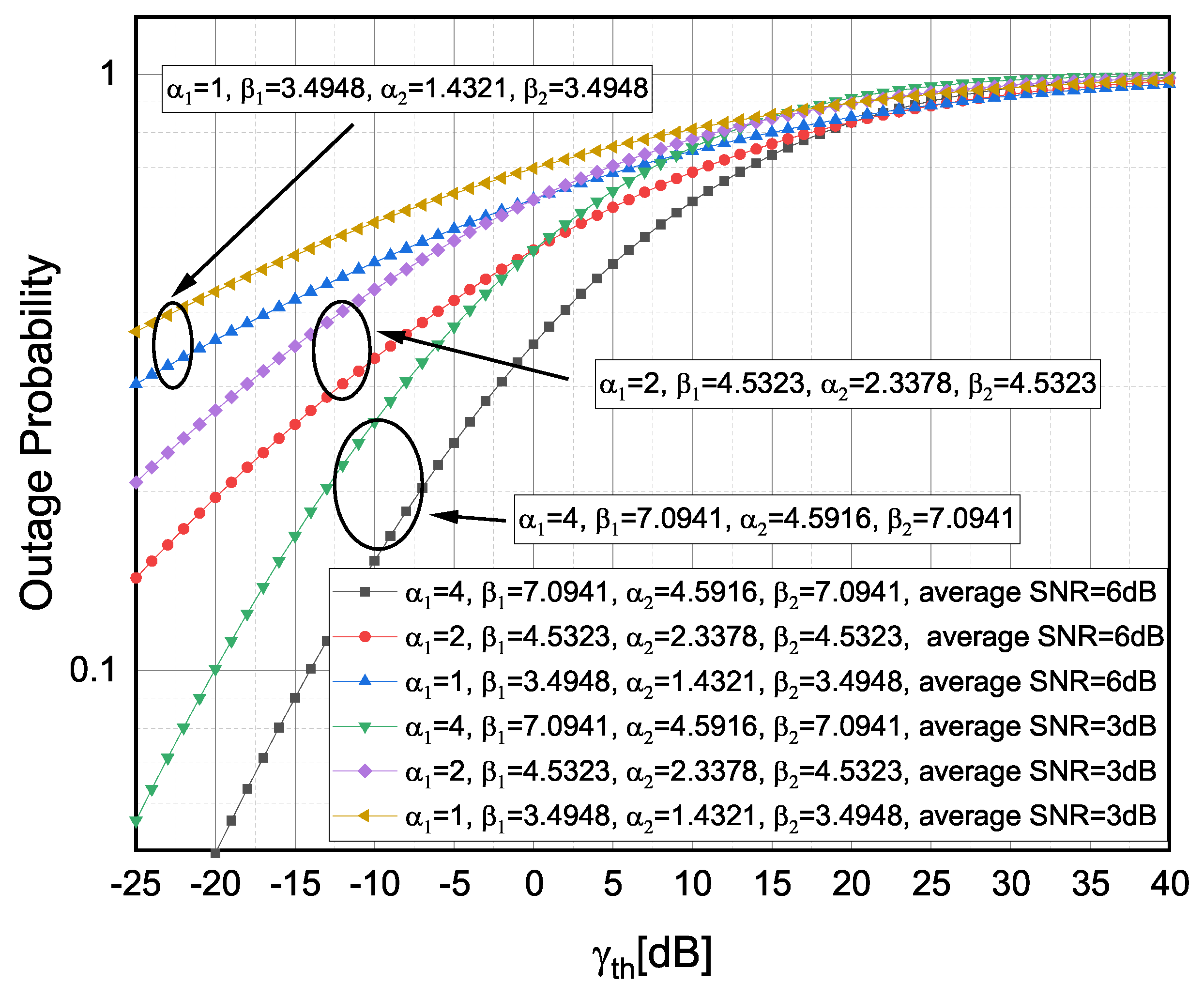
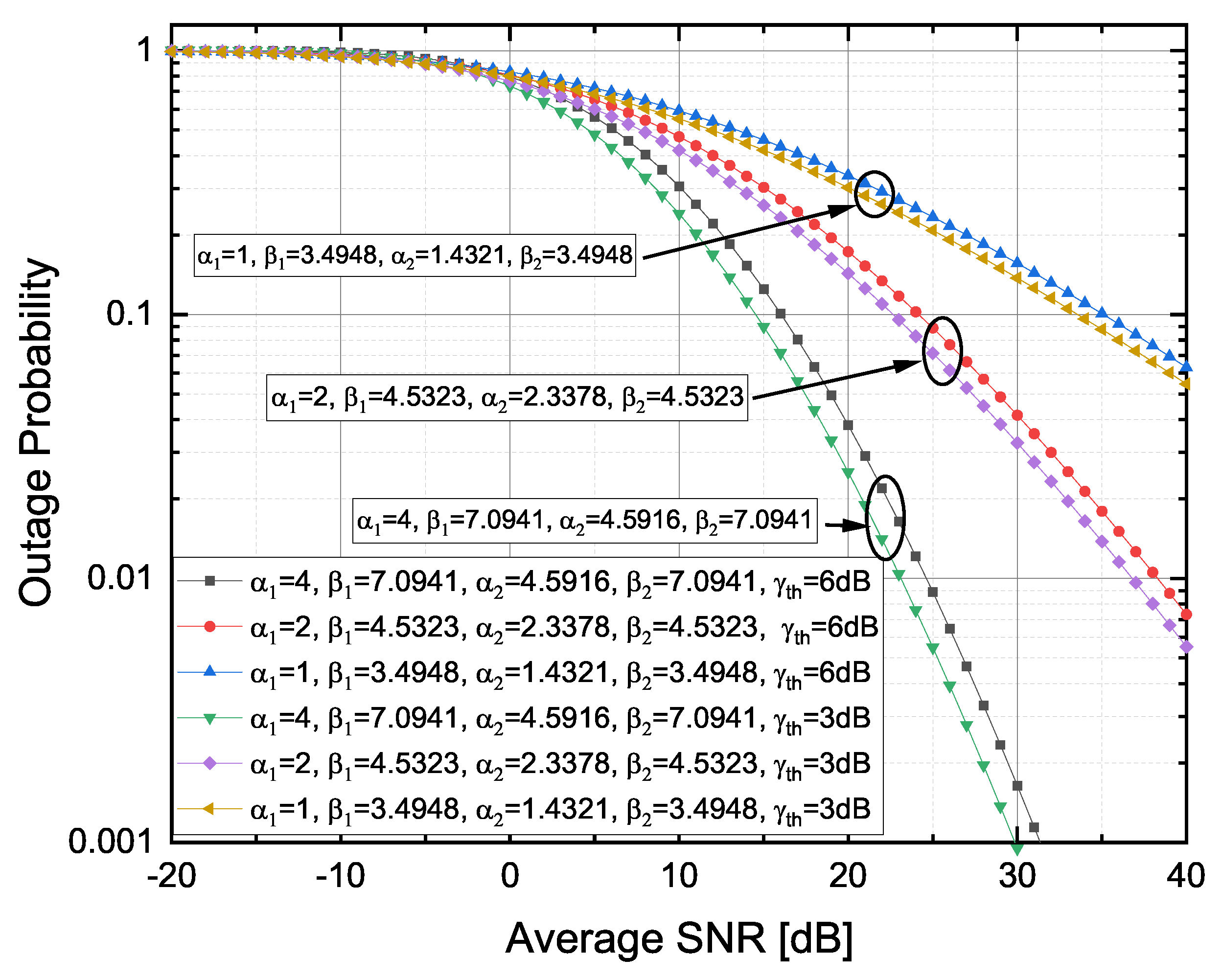
The OP versus $\gamma$ as well as the OP versus $\overline{\gamma }$ for weak $(a_1=5,b_1=7.0941,a_2=4.5916,b_2=7.0941)$, moderate $(a_1=2,b_1=4.5323,a_2=2.3378,b_2=4.5323)$ and strong $(a_1=1,b_1=3.4948,a_2=1.4321,b_2=3.4948)$ TI fading severities [14] are presented, respectively, in Figure 2 and Figure 3. Since (23) was the C-F finite series expression, the presented numerical results for the OP were limited to integer values of $a_1$. It can be observed that, by shifting from strong-to-moderate or moderate-to-weak TI fading conditions, the OP decreased. In Figure 2, it can be further noticed that, by increasing the average SNR values, the OP decreased, which in turn could provide an additional system performance improvement of the FSO RIS-ACs link over F-S TI fading propagation channels. From Figure 3, it can be observed that a higher $\overline{\gamma }$ caused an increase in the OP (e.g., by increasing $\overline{\gamma }$ from $\overline{\gamma }=3$ to $\overline{\gamma }=6$).

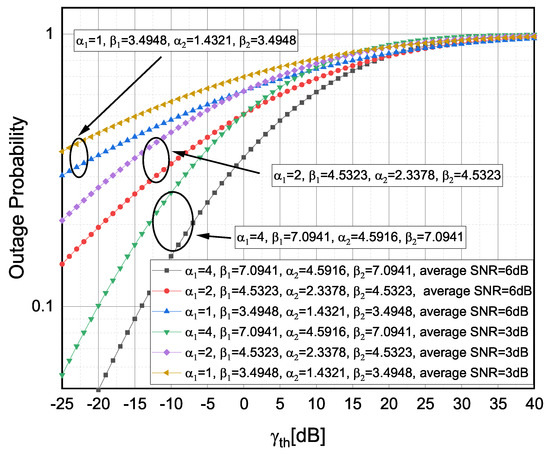
Figure 2. Outage probability versus ${\gamma }_{th}$ observed for different TI fading severity conditions.

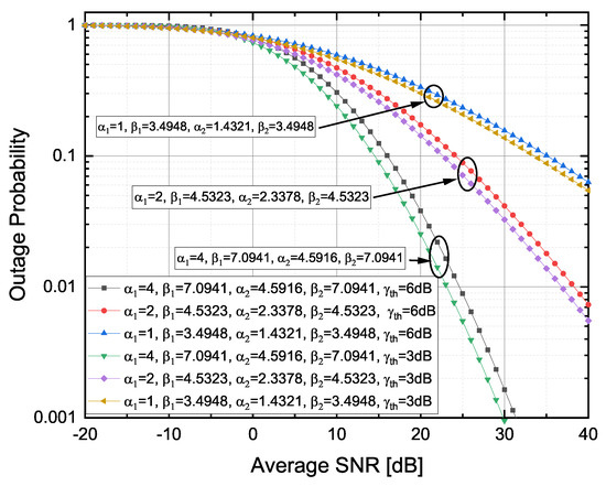
Figure 3. Outage probability versus $\overline{{\gamma }_{th}}$ observed for different TI fading severity conditions.

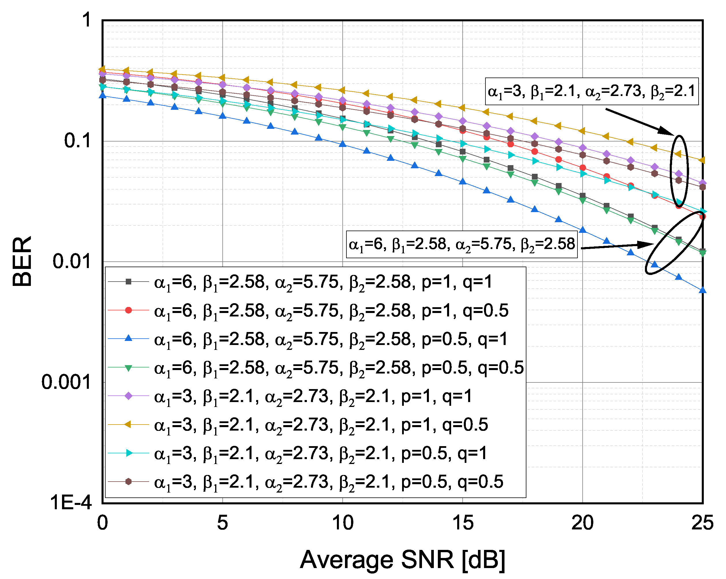
The $P_{BER}(\gamma )$ versus $\overline{\gamma }$ for $a_1=6,b_1=2.58,a_2=5.75,b_2=2.58$ and $a_1=3,b_1=2.1,a_2=2.73$ and $b_2=2.1$ TI fading severity values [13], where $a_1$ was an integer, and for the selected binary modulation schemes such as BFSK, BPSK, NBFSK and DBPSK are presented in Figure 4. It was obvious that less severe TI fading conditions provided a lower $P_{BER}(\gamma )$ (e.g., by shifting from $a_1=3,b_1=2.1,a_2=2.73$ and $b_2=2.1$ to $a_1=6,b_1=2.58,a_2=5.75$ and $b_2=2.58$). It can be further concluded that, for higher dB $\overline{\gamma }$ values, TI fading conditions had a stronger impact on the $P_{BER}(\gamma )$ than the observed modulation schemes.

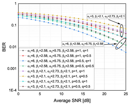
Figure 4. Average BER versus $\overline{{\gamma }_{th}}$ observed for different TI fading severity conditions and different modulations technique.

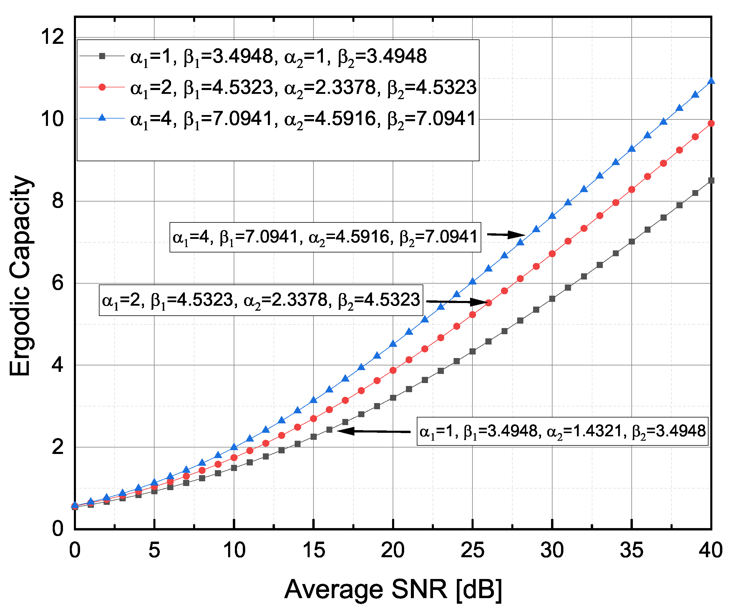
The $C_{\gamma }$ of the considered FSO RIS-ACs model over F-S $\mathcal{F}$ TI fading propagation channels for weak $(a_1=4,b_1=7.0941,a_2=4.5916,b_2=7.0941)$, moderate $(a_1=2,b_1=4.5323,a_2=2.3378,b_2=4.5323)$ and strong $(a_1=1,b_1=3.4948,a_2=1.4321,b_2=3.4948)$ TI fading severities [14], where $a_1$ took integer values, is shown in Figure 5. As expected, the $C_{\gamma }$ could be increased by shifting from severe to less severe TI fading conditions (e.g., by shifting from strong-to-moderate or moderate-to-weak TI fading severities). A similar behaviour for an FSO RIS AC under the IM–DD modulation technique was noticed in [24,27].

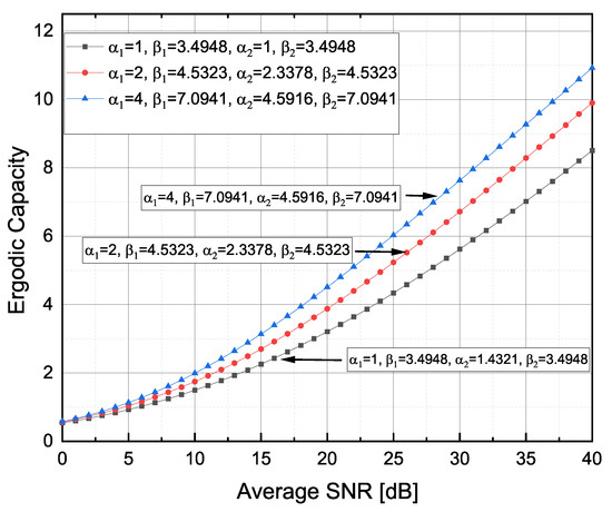
Figure 5. Ergodic capacity versus $\overline{{\gamma }_{th}}$ observed for different TI fading severity conditions.

6.2. Numerical Results for S-O Performance Metrics

The S-O statistical measures of an FSO RIS-ACs model over F-S $\mathcal{F}$ TI fading propagation channels are presented in Figure 6 and Figure 7. The variances in (40) were evaluated as ${\sigma }_{{\gamma }_{h_1}}^2={\sigma }_{{\gamma }_{h_2}}^2={f_0}^2{\pi }^2{\sigma }_{{\gamma }_h}^2⟨{\gamma }_h⟩$ ([30], Equation (13)), where ${\sigma }_{{\gamma }_h}^2={\sigma }_{{\gamma }_{h_i}}^2$ was given by (11) and $⟨{\gamma }_h⟩=⟨{\gamma }_{h_i}⟩=1$. Furthermore, $f_0=\frac{1}{\pi {\tau }_0\sqrt{2}}$ was the quasi frequency of the FSO RIS-ACs path ([30], Equation (15)). Additionally, ${\tau }_0=\frac{\sqrt{\lambda S}}{U}$ was the turbulence correlation time, $\lambda$ was the wavelength, S was the distance and U was the average wind speed of the RIS-ACs transmission system. The S-O metrics were evaluated for $\lambda ={\lambda }_i=532$ nm, $U=1$ m/s and $S=980$ m [46].

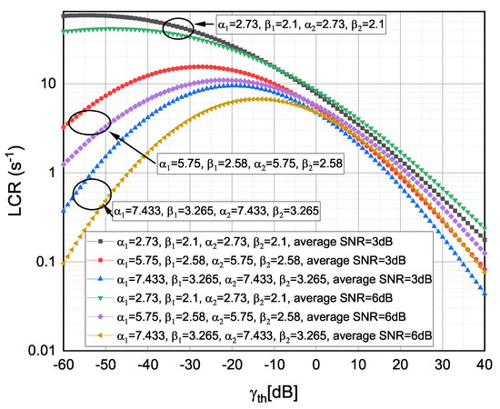
Figure 6. Average level crossing rate versus ${\gamma }_{th}$ observed for different TI fading severity conditions and different $\overline{{\gamma }_{th}}$.

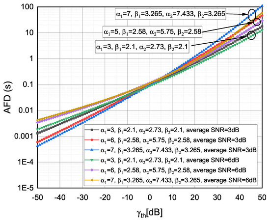
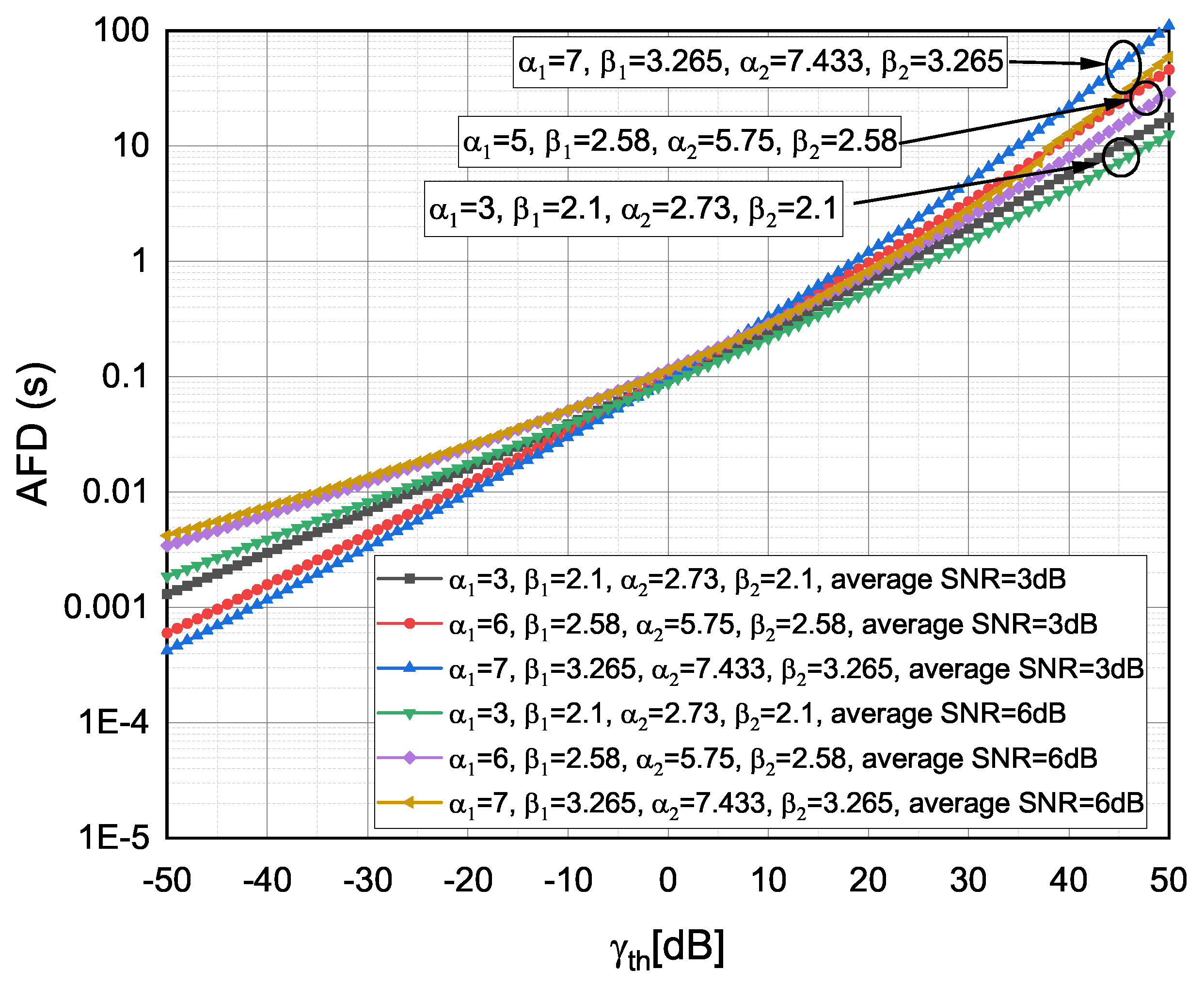
Figure 7. Average fade duration versus ${\gamma }_{th}$ observed for different TI fading severity conditions and different $\overline{{\gamma }_{th}}$.

The $N_{\gamma }$ versus ${\gamma }_{th}$ for weak $(a_1=7.433,b_1=3.265,a_2=7.433,b_2=3.265)$, moderate $(a_1=5.75,b_1=2.58,a_2=5.75,b_2=2.58)$ and strong $(a_1=2.7,b_1=2.1,a_2=2.73,b_2=2.1)$ TI fading severity values [13] and for various ${\overline{\gamma }}_{th}$ values is presented in Figure 6. The least severe (observed) TI fading conditions providing the lowest $N_{\gamma }({\gamma }_{th})$ values throughout the ${\gamma }_{th}$ dB regime (e.g., the lowest $N_{\gamma }({\gamma }_{th})$ values were obtained for $a_1=7.433,b_1=3.265,a_2=7.433$ and $b_2=3.265$ TI fading severities). As expected, the shifts from more severe to less severe TI fading conditions cause the $N_{\gamma }({\gamma }_{th})$ to decrease. The increase in ${\overline{\gamma }}_{th}$ (e.g., by increasing $\overline{\gamma }$ from $\overline{\gamma }=3$ to $\overline{\gamma }=6$) could caused $N_{\gamma }({\gamma }_{th})$ to decrease for lower ${\gamma }_{th}$ dB values and $N_{\gamma }({\gamma }_{th})$ to slightly increase for higher ${\gamma }_{th}$ dB values. It was also evident that the impact of TI fading severities on $N_{\gamma }({\gamma }_{th})$ was more dominant for lower ${\gamma }_{th}$ dB values.

The $A_{\gamma }({\gamma }_{th})$ for weak $(a_1=7,b_1=3.265,a_2=7.433,b_2=3.265)$, moderate $(a_1=6,b_1=2.58,a_2=5.75,b_2=2.58)$ and strong $(a_1=3,b_1=2.1,a_2=2.73,b_2=2.1)$ TI fading severity values [13], where $a_1$ was an integer, and for various ${\overline{\gamma }}_{th}$ values, is presented in Figure 7. It can be observed that, by shifting from less severe to more severe TI fading conditions, the $A_{\gamma }({\gamma }_{th})$ decreased for higher ${\gamma }_{th}$ dB values (e.g., by shifting from $a_1=7,b_1=3.265,a_2=7.433$ and $b_2=3.265$ to $a_1=6,b_1=2.58,a_2=5.75$ and $b_2=2.58$ or from $a_1=6,b_1=2.58,a_2=5.75$ and $b_2=2.58$ to $a_1=3,b_1=2.1,a_2=2.73$ and $b_2=2.1$). It can be further noticed that $\overline{\gamma }$ had a stronger impact on $A_{\gamma }({\gamma }_{th})$ for smaller ${\gamma }_{th}$ dB values, while TI fading severity conditions had a stronger impact on $A_{\gamma }({\gamma }_{th})$ for higher ${\gamma }_{th}$ dB values. Moreover, the $A_{\gamma }({\gamma }_{th})$ was the least affected by TI fading severity conditions and $\overline{\gamma }$ for the threshold values around ${\gamma }_{th}=0$ dB.

7. Conclusions

The unified F-O and S-O performance analysis of an FSO RIS-ACs over F-S $\mathcal{F}$ TI fading channels under different TI fading severity conditions was investigated. Namely, novel C-F expressions for $p_{\gamma }(\gamma )$ and $F_{\gamma }(\gamma )$ of the received SNR in terms of Beta and Gauss-hypergeometric functions were successfully derived. The $F_{\gamma }(\gamma )$ was obtained as a finite series expression and, as such, was only valid for integer values of $a_1$. Capitalizing on the obtained analytical expressions for $p_{\gamma }(\gamma )$ and $F_{\gamma }(\gamma )$, the novel C-F expressions of the end-to-end SNR for ${\mathcal{M}}_{MGF}$, $P_{\gamma }({\gamma }_{th})$, $P_{BER}(\gamma )$ and $C_{\gamma }$ in terms of the Meijer G function were derived and numerically evaluated for different F-S $\mathcal{F}$ TI fading system model parameters. Moreover, the paper provided the mathematical framework for the derivation of S-O statistical measures such as $N_{\gamma }({\gamma }_{th})$ and $A_{\gamma }({\gamma }_{th})$ of an FSO RIS-ACs system over F-S $\mathcal{F}$ TI fading channels under different TI fading severity conditions. The obtained results pointed out that a significant performance improvement of SISO FSO RIS-ACs links could be achieved by shifting from more severe to less severe TI fading conditions. Moreover, the system performance improvement in terms of $P_{\gamma }({\gamma }_{th})$ could be further achieved by increasing the $\overline{\gamma }$ dB value. The provided analytical and numerical results could be useful for designing SISO FSO RIS-ACs systems over TI fading channels. Further works will consider the experimental validation of the obtained results.

References

- Alghamdi, R.; Alhadrami, R.; Alhothali, D.; Almorad, H.; Faisal, A.; Helal, S.; Shalabi, R.; Asfour, R.; Hammad, N.; Shams, A.; et al. Intelligent surfaces for 6G wireless networks: A survey of optimization and performance analysis techniques. IEEE Access 2020, 8, 202795–202818. [Google Scholar] [CrossRef]
- Liu, Y.; Liu, X.; Mu, X.; Hou, T.; Xu, J.; Di Renzo, M.; Al-Dhahir, N. Reconfigurable intelligent surfaces: Principles and opportunities. IEEE Commun. Surv. Tutor. 2021, 23, 1546–1577. [Google Scholar] [CrossRef]
- Di Renzo, M.; Zappone, A.; Debbah, M.; Alouini, M.-S.; Yuen, C.; De Rosny, J.; Tretyakov, S. Smart Radio Environments Empowered by Reconfigurable Intelligent Surfaces: How It Works, State of Research, and The Road Ahead. IEEE J. Sel. Areas Commun. 2020, 38, 2450–2525. [Google Scholar] [CrossRef]
- Tang, W.; Chen, M.Z.; Chen, X.; Dai, J.Y.; Han, Y.; Di Renzo, M.; Zeng, Y.; Jin, S.; Cheng, Q.; Cui, T.J. Wireless communications with reconfigurable intelligent surface: Path loss modeling and experimental measurement. IEEE Trans. Wirel. Commun. 2021, 20, 421–439. [Google Scholar] [CrossRef]
- Di Renzo, M.; Ntontin, K.; Song, J.; Danufane, F.H.; Qian, X.; Lazarakis, F.; De Rosny, J.; Phan-Huy, D.T.; Simeone, O.; Zhang, R.; et al. Reconfigurable intelligent surfaces vs. relaying: Differences, similarities, and performance comparison. IEEE Open J. Commun. Soc. 2020, 1, 798–807. [Google Scholar] [CrossRef]
- Perović, N.; Di Renzo, M.; Flanagan, F. Channel Capacity Optimization Using Reconfigurable Intelligent Surfaces in Indoor mmWave Environments. In Proceedings of the ICC 2020—2020 IEEE International Conference on Communications (ICC), Dublin, Ireland, 7–11 June 2020; pp. 1–7. [Google Scholar]
- Abumarshoud, H.; Mohjazi, L.; Dobre, O.A.; Di Renzo, M.; Imran, M.A.; Haas, H. LiFi Through Reconfigurable Intelligent Surfaces: A New Frontier for 6G? arXiv 2021, arXiv:2104.02390. [Google Scholar]
- Ndjiongue, A.R.; Ngatched, T.M.N.; Dobre, O.A.; Haas, H. Re-configurable Intelligent Surface-based VLC Receivers Using Tunable Liquid-crystals: The Concept. J. Lightwave Technol. 2021, 39, 3193–3200. [Google Scholar] [CrossRef]
- Al-Habash, A.; Andrews, L.C.; Phillips, R.L. Mathematical model for the irradiance probability density function of a laser beam propagating through turbulent media. Opt. Eng. 2001, 40, 1554–1562. [Google Scholar] [CrossRef]
- Bayaki, E.; Schober, R.; Mallik, R. Performance analysis of MIMO free-space optical systems in gamma-gamma fading. IEEE Trans. Commun. 2009, 57, 3415–3424. [Google Scholar] [CrossRef]
- Moradi, H.; Falahpour, M.; Refai, H.H.; LoPresti, P.G.; Atiquzzaman, M. BER analysis of optical wireless signals through lognormal fading channels with perfect CSI. In Proceedings of the 17th International Conference on Telecommunications, Bali, Indonesia, 7–11 June 2010; pp. 493–497. [Google Scholar]
- Ansari, I.S.; Yilmaz, F.; Alouini, M.-S. Performance Analysis of Free-Space Optical Links Over Málaga (M) Turbulence Channels With Pointing Errors. IEEE Trans. Wirel. Commun. 2016, 15, 91–102. [Google Scholar] [CrossRef] [Green Version]
- Peppas, K.P.; Alexandropoulos, G.C.; Xenos, E.D.; Maras, A. The Fischer–Snedecor F-Distribution Model for Turbulence-Induced Fading in Free-Space Optical Systems. J. Lightwave Technol. 2020, 38, 1286–1295. [Google Scholar] [CrossRef]
- Badarneh, O.S.; Derbas, R.; Almehmadi, F.S.; El Bouanani, F.; Muhaidat, S. Performance Analysis of FSO Communications Over F Turbulence Channels With Pointing Errors. IEEE Commun. Lett. 2021, 25, 926–930. [Google Scholar] [CrossRef]
- Badarneh, O.S.; Mesleh, R. Diversity analysis of simultaneous mmWave and free-space-optical transmission over F-distribution channel models. J. Opt. Commun. Netw. 2020, 12, 324–334. [Google Scholar] [CrossRef]
- Han, L.; Wang, Y.; Liu, X.; Li, B. Secrecy performance of FSO using HD and IM/DD detection technique over F-distribution turbulence channel with pointing error. IEEE Commun. Lett. 2021, 10, 2245–2248. [Google Scholar] [CrossRef]
- Yoo, S.K.; Cotton, S.L.; Sofotasios, P.C.; Matthaiou, M.; Valkama, M.; Karagiannidis, G.K. The Fisher–Snedecor F Distribution: A Simple and Accurate Composite Fading Model. IEEE Commun. Lett. 2017, 21, 1661–1664. [Google Scholar] [CrossRef] [Green Version]
- Maričić, S.; Milošević, N.; Drajić, D.; Milić, D.; Anastasov, J. Physical Layer Intercept Probability in Wireless Sensor Networks over Fisher—Snedecor F Fading Channels. Electronics 2021, 10, 1368. [Google Scholar] [CrossRef]
- Zhang, J.; Du, H.; Sun, Q.; Ai, B.; Ng, D.W.K. Physical Layer Security Enhancement With Reconfigurable Intelligent Surface-Aided Networks. IEEE Trans. Inf. Forensics Secur. 2021, 16, 3480–3495. [Google Scholar] [CrossRef]
- Anastasov, J.A.; Cvetkovic, A.M.; Milic, D.N.; Djordjevic, G.; Milovic, D. Noisy Reference Loss for PSK Signal Detection over Fisher-Snedecor F Fading Channel. In Proceedings of the 17th International Conference on Telecommunications, Sirince, Turkey, 7–11 June 2010; pp. 493–497. [Google Scholar]
- Makarfi, A.; Rabie, K.; Kaiwartya, O.; Badarneh, O.; Nauryzbayev, G.; Kharel, R. Physical Layer Security in RIS-assisted Networks in Fisher-Snedecor Composite Fading. In Proceedings of the 12th International Symposium on Communication Systems, Networks and Digital Signal Processing (CSNDSP), Porto, Portugal, 20–22 July 2020. [Google Scholar]
- Yoo, S.K.; Cotton, S.L.; Sofotasios, P.C.; Muhaidat, S.; Karagiannidis, G.K. Level Crossing Rate and Average Fade Duration in F Composite Fading Channels. IEEE Wirel. Commun. Lett. 2020, 9, 281–284. [Google Scholar] [CrossRef]
- Cheng, W.; Wang, X. Bivariate Fisher–Snedecor F Distribution and its Applications in Wireless Communication Systems. IEEE Access 2020, 8, 146342–146360. [Google Scholar] [CrossRef]
- Ndjiongue, A.R.; Ngatched, T.; Dobre, O.; Armada, A.G.; Haas, H. Analysis of RIS-Based Terrestrial-FSO Link over G-G Turbulence with Distance and Jitter Ratios. J. Lightwave Technol. 2021, 39, 6746–6758. [Google Scholar] [CrossRef]
- Yang, L.; Guo, W.; Ansari, I.S. Mixed dual-hop FSO-RF communication systems through reconfigurable intelligent surface. IEEE Commun. Lett. 2020, 24, 1558–1562. [Google Scholar] [CrossRef]
- Najafi, M.; Schmauss, B.; Schober, R. Intelligent Reflecting Surfaces for Free Space Optical Communication Systems. IEEE Trans. Commun. 2021, 69, 6134–6151. [Google Scholar] [CrossRef]
- Chapala, V.K.; Zafaruddin, S.M. Unified Performance Analysis of Reconfigurable Intelligent Surface Empowered Free Space Optical Communications. arXiv 2021, arXiv:2106.02000. [Google Scholar]
- Vetelino, F.S.; Young, C.; Andrews, L. Fade statistics and aperture averaging for Gaussian beam waves in moderate-to-strong turbulence. Appl. Opt. 2007, 46, 3780–3789. [Google Scholar] [CrossRef]
- Kim, K.H.; Higashino, T.; Tsukamoto, K.; Komaki, S. Optical fading analysis considering spectrum of optical scintillation in terrestrial free-space optical channel. In Proceedings of the IEEE International Conference on Space Optical Systems and Applications, Santa Monica, CA, USA, 11–13 May 2011; pp. 58–66. [Google Scholar]
- Jurado-Navas, A.; Garrido-Balsells, J.M.; Castillo-Vázquez, M.; Puerta-Notario, A.; Monroy, I.T.; Olmos, J.J. Fade statistics of M-turbulent optical links. EURASIP J. Wirel. Commun. Netw. 2017, 112, 1–9. [Google Scholar]
- Stefanović, C.; Panić, S.; Djosić, D.; Milić, D.; Stefanović, M. On the second order statistics of N-hop FSO communications over N-gamma-gamma turbulence induced fading channels. Phys. Commun. 2021, 45, 101289. [Google Scholar] [CrossRef]
- Issaid, C.B.; Alouini, M.S. Level Crossing Rate and Average Outage Duration of Free Space Optical Links. IEEE Trans. Commun. 2019, 67, 6234–6242. [Google Scholar] [CrossRef] [Green Version]
- Stefanovic, C.; Céspedes, M.M.; Roka, R.; Armada, A.G. Performance analysis of N-Fisher-Snedecor F fading and its application to N-hop FSO communications. In Proceedings of the 17th IEEE International Symposium on Wireless Communication Systems (ISWCS), Berlin, Germany, 6–9 September 2021. [Google Scholar]
- Le, H.D.; Pham, A.T. Level Crossing Rate and Average Fade Duration of Satellite-to-UAV FSO Channels. IEEE Photonics J. 2021, 13, 1–14. [Google Scholar] [CrossRef]
- Stefanovic, C.; Pratesi, M.; Santucci, F. Second order statistics of mixed RF-FSO relay systems and its application to vehicular networks. In Proceedings of the IEEE International Conference on Communications (ICC), Shanghai, China, 20–24 May 2019. [Google Scholar]
- Waseer, W.I.; Nawaz, S.J.; Gulfam, S.M.; Mughal, M.J. Second-order fading statistics of massive-MIMO vehicular radio communication channels. Trans. Emerg. Telecommun. Technol. 2018, 29, e3487. [Google Scholar] [CrossRef]
- Stefanovic, C.; Panic, S.; Bhatia, V.; Kumar, N. On second-order statistics of the composite channel models for UAV-to-ground communications with UAV selection. IEEE Open J. Commun. Soc. 2021, 2, 534–544. [Google Scholar] [CrossRef]
- Le, H.D.; Mai, V.V.; Nguyen, C.T.; Pham, A.T. Design and analysis of sliding window arq protocols with rate adaptation for burst transmission over fso turbulence channels. J. Opt. Commun. Netw. 2019, 11, 151–163. [Google Scholar] [CrossRef]
- Gradshteyn, I.S.; Ryzhik, I.M. The title of the cited contribution. In Table of Integrals, Series, and Products; Academic: New York, NY, USA, 2000. [Google Scholar]
- Yigit, Z.; Basar, E.; Altunbas, I. Low complexity adaptation for reconfigurable intelligent surface-based MIMO systems. IEEE Commun. Lett. 2020, 24, 2946–2950. [Google Scholar] [CrossRef]
- Wolfram Research Inc. The Mathematical Functions Site; Wolfram Research, Inc.: Champaign, IL, USA, 2010; Available online: https://functions.wolfram.com/ (accessed on 1 September 2021).
- Petkovic, M.; Cvetkovic, M.; Djordjevic, G.T.; Karagiannidis, G.K. Partial Relay Selection With Outdated Channel State Estimation in Mixed RF/FSO Systems. J. Lightwave Technol. 2015, 33, 2860–2867. [Google Scholar] [CrossRef]
- Lopez-Martinez, F.J.; Kurniawan, E.; Islam, R.; Goldsmith, A. Average fade duration for amplify-and-forward relay networks in fading channels. IEEE Trans. Wirel. Commun. 2015, 14, 5454–5467. [Google Scholar] [CrossRef]
- Chau, Y.A.; Huang, K.Y.-T. Burst-error analysis of dual-hop fading channels based on the second-order channel statistics. IEEE Trans. Veh. Technol. 2010, 59, 3108–3115. [Google Scholar] [CrossRef]
- Hadzi-Velkov, Z.; Zlatanov, N.; Karagiannidis, G.K. On the second order statistics of the multihop Rayleigh fading channel. IEEE Trans. Commun. 2009, 33, 2860–2867. [Google Scholar] [CrossRef]
- Wayne, D.T. The PDF of Irradiance for a Free-Space Optical Communications Channel: A Physics Based Model. Ph.D. Thesis, College of Engineering and Computer Science, University of Central Florida, Orlando, FL, USA, 2010. [Google Scholar]
Publisher’s Note: MDPI stays neutral with regard to jurisdictional claims in published maps and institutional affiliations. |
© 2021 by the authors. Licensee MDPI, Basel, Switzerland. This article is an open access article distributed under the terms and conditions of the Creative Commons Attribution (CC BY) license (https://creativecommons.org/licenses/by/4.0/).