
Bottom-Up Model of Random Daily Electrical Load Curve for Office Building

Abstract
:1. Introduction
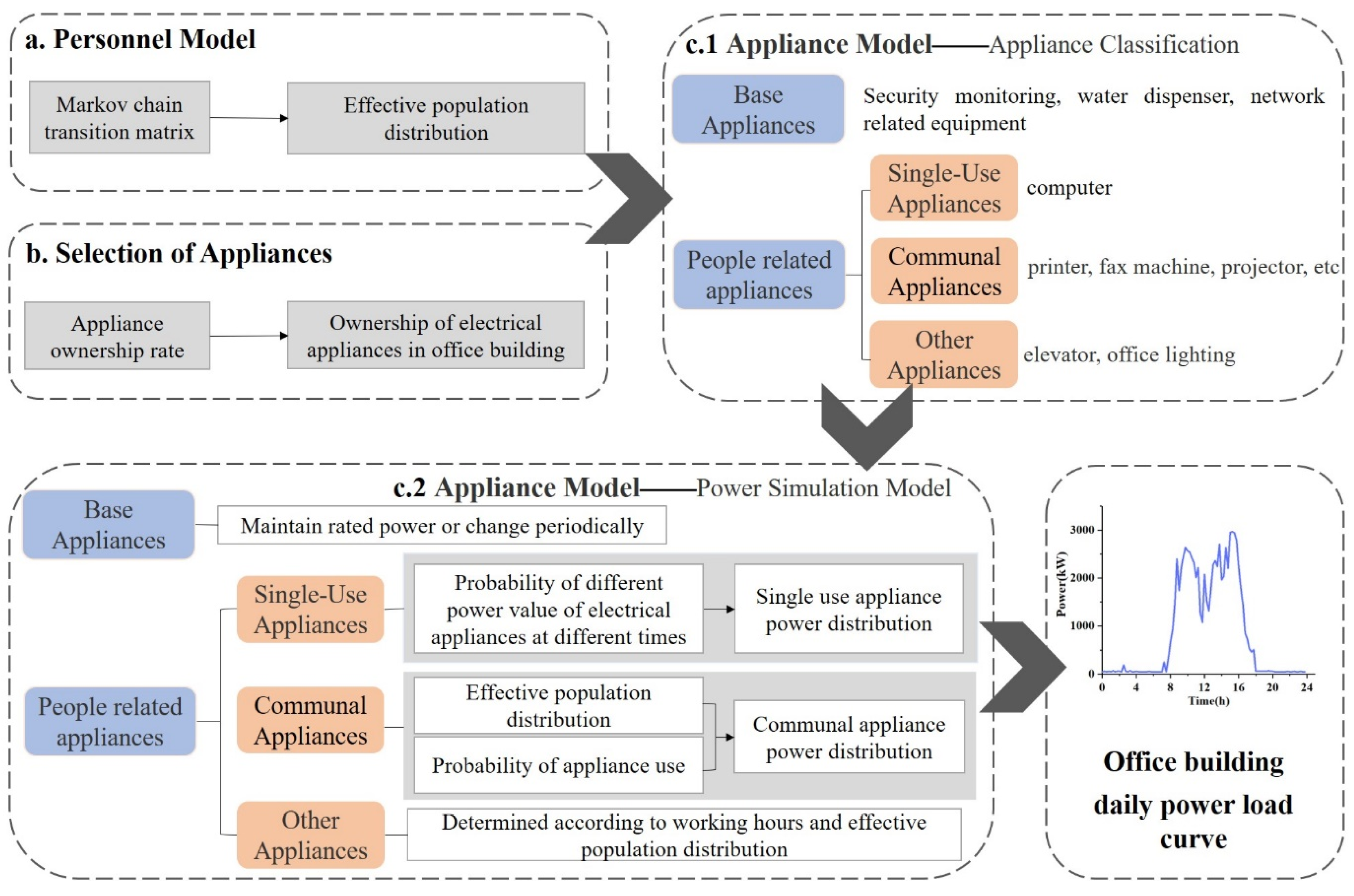
2. Modeling Approach
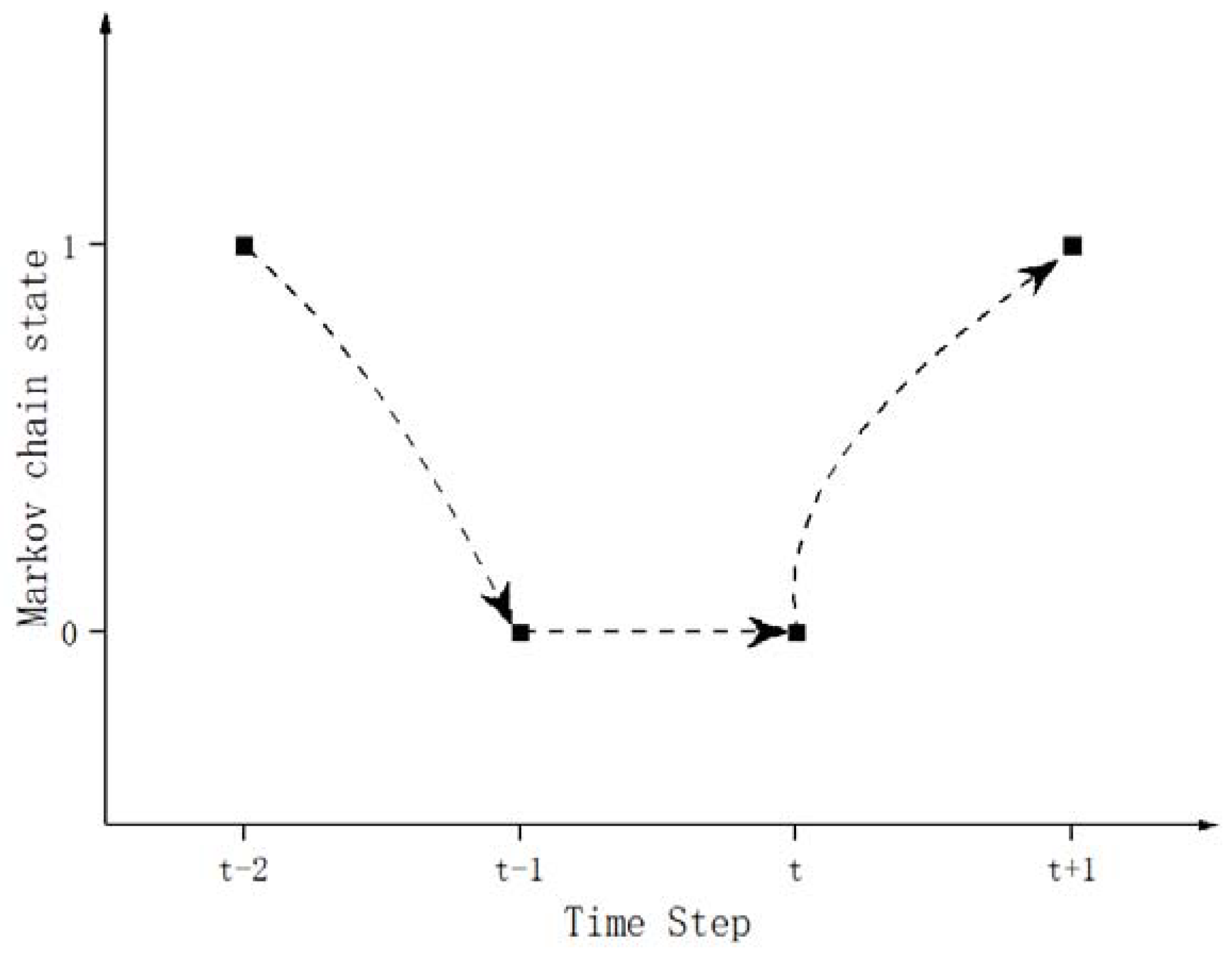
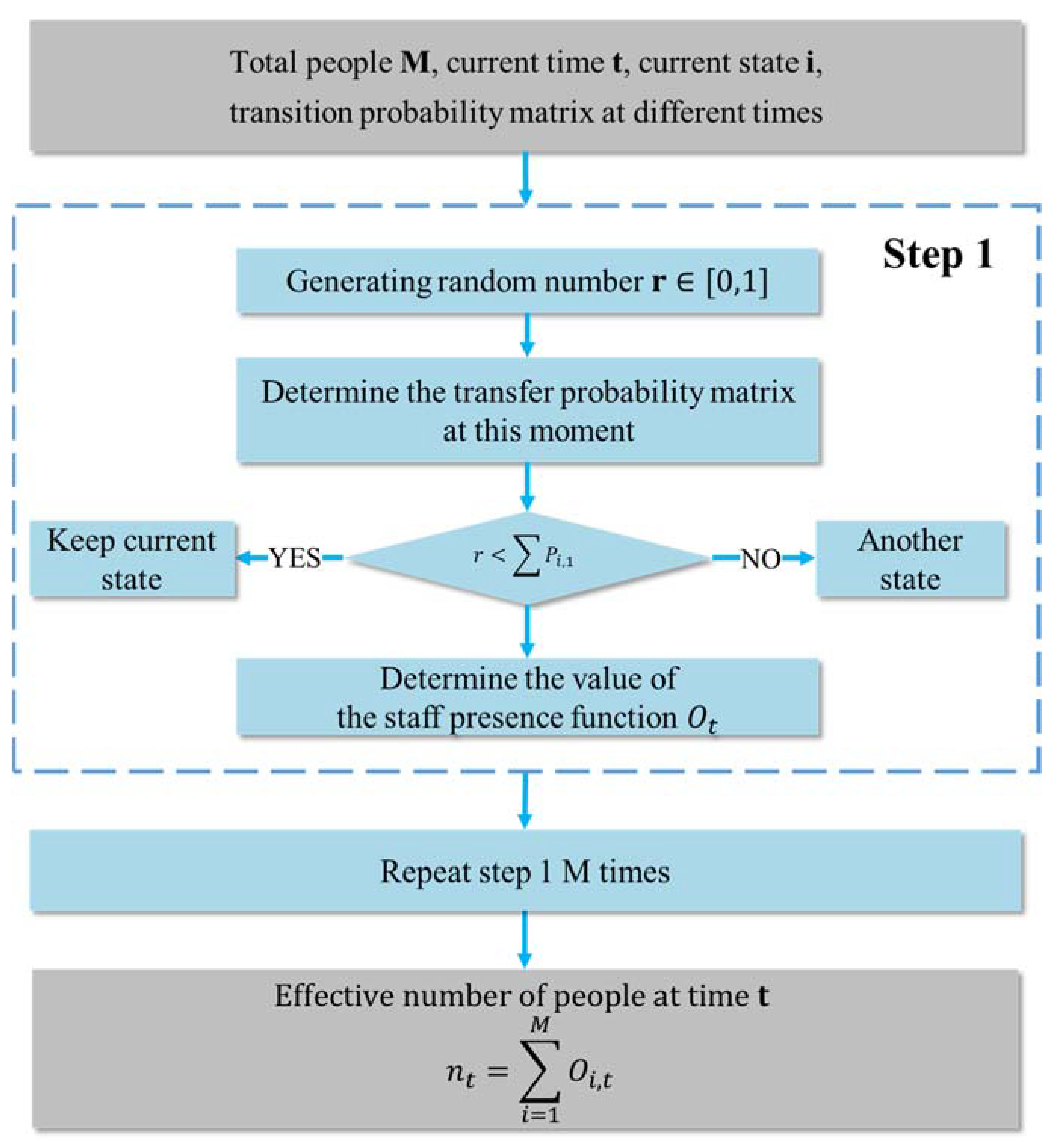
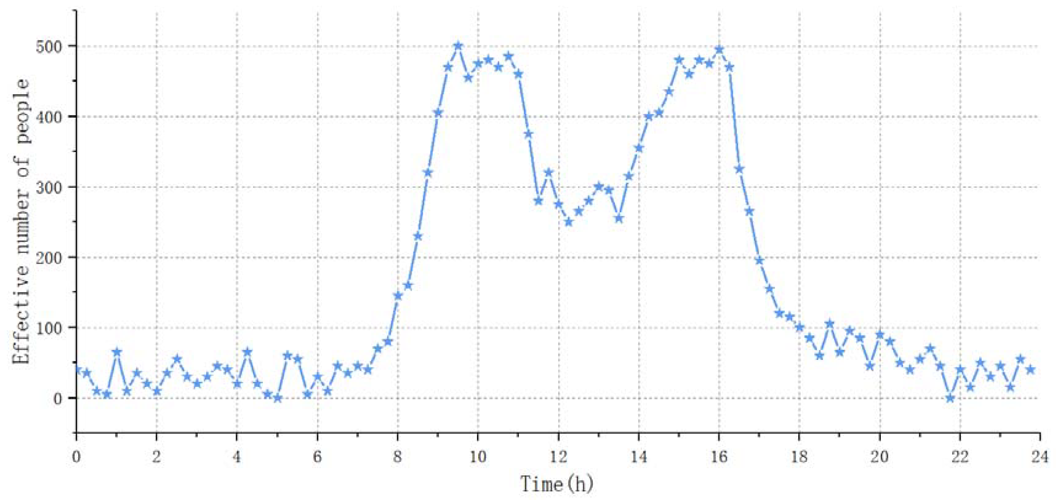
2.1. Personnel Model
- Enter the total number of people M, the current time t, the current state i, and the transition probability matrix at different times;
- Randomly sample the number r between 0 and 1 in each time step and compare it with the transition probability to determine the status of the person in the room;
- Determine the effective number of people in the office building by performing the entire sequence of random sampling M times.
2.2. Selection of Appliances
2.3. Appliance Model
2.3.1. Appliance Classification
- (i)
- Base Appliances: the behavior of indoor personnel has nothing to do with the power value, and the rated power is always maintained, such as security monitoring, or the power value changes periodically, such as water dispenser.
- (ii)
- Single-Use Appliances: appliances owned by every person in the room, such as computer.
- (iii)
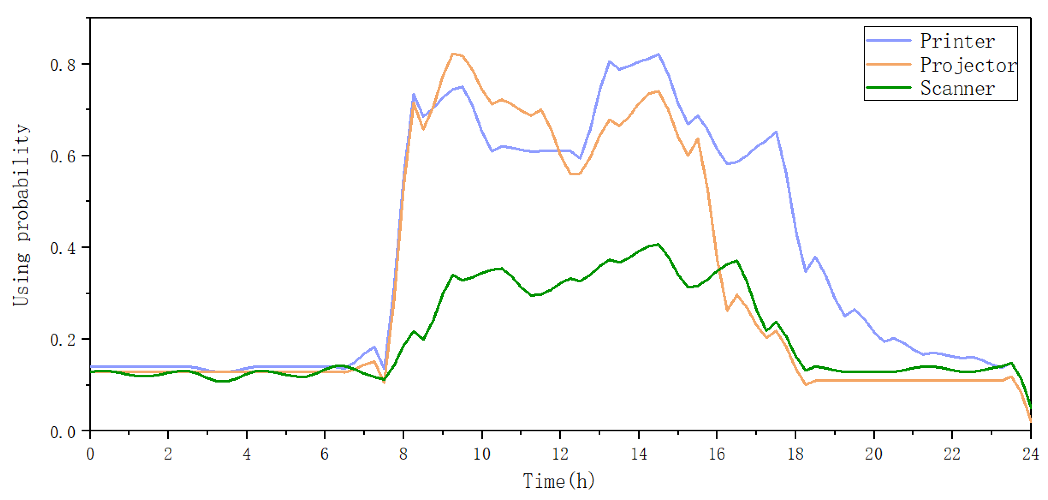
- Communal Appliances: appliances shared by at least two or more people, such as printer, projector, paper shredder, etc.
- (iv)
- Other Appliances: in addition to the above types of electrical appliances, other electrical appliances related to work and rest time and the number of indoor personnel, such as elevators and office lighting.
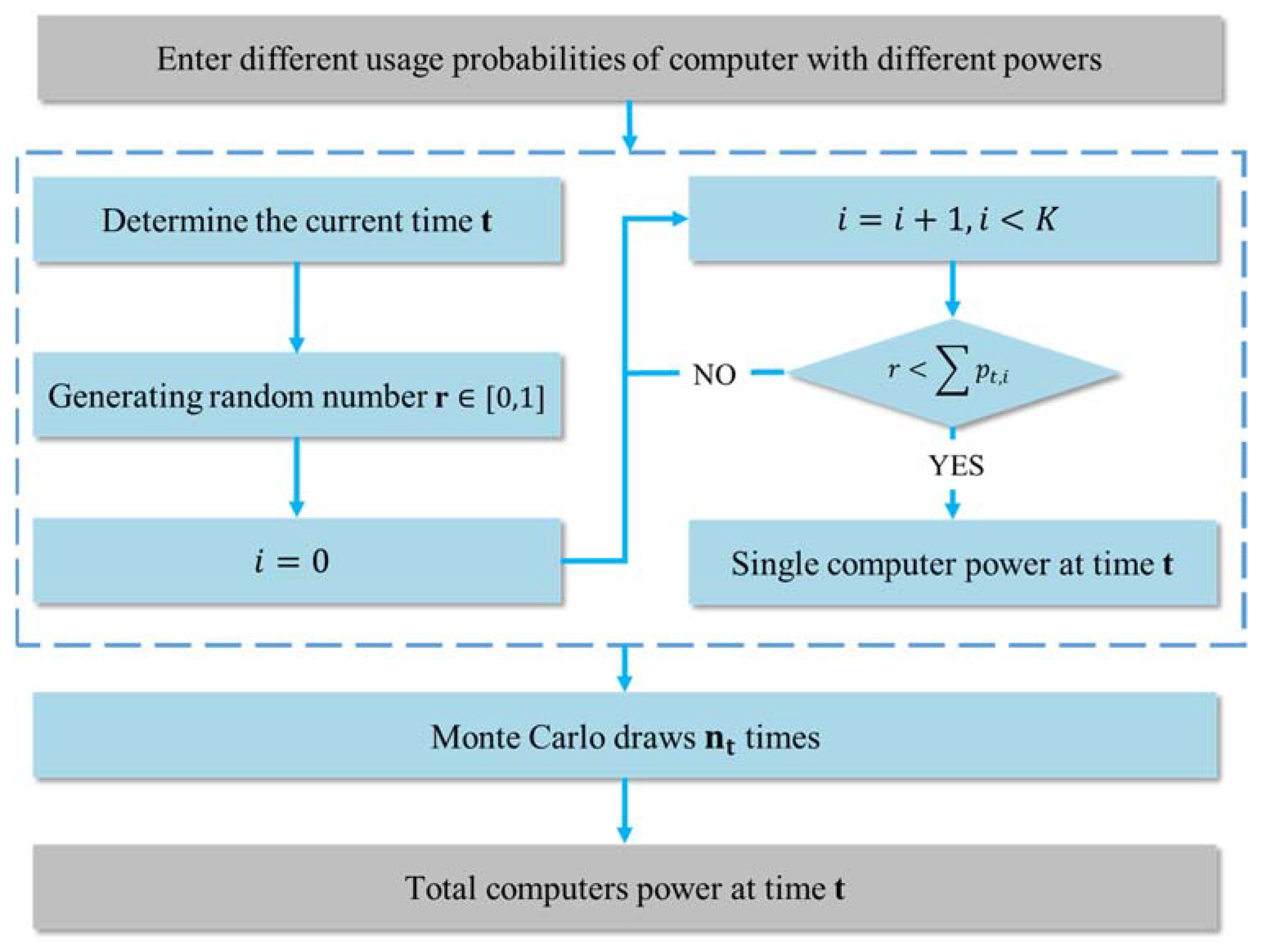
2.3.2. Power Simulation Model
- (i)
- Base Appliances
- (ii)
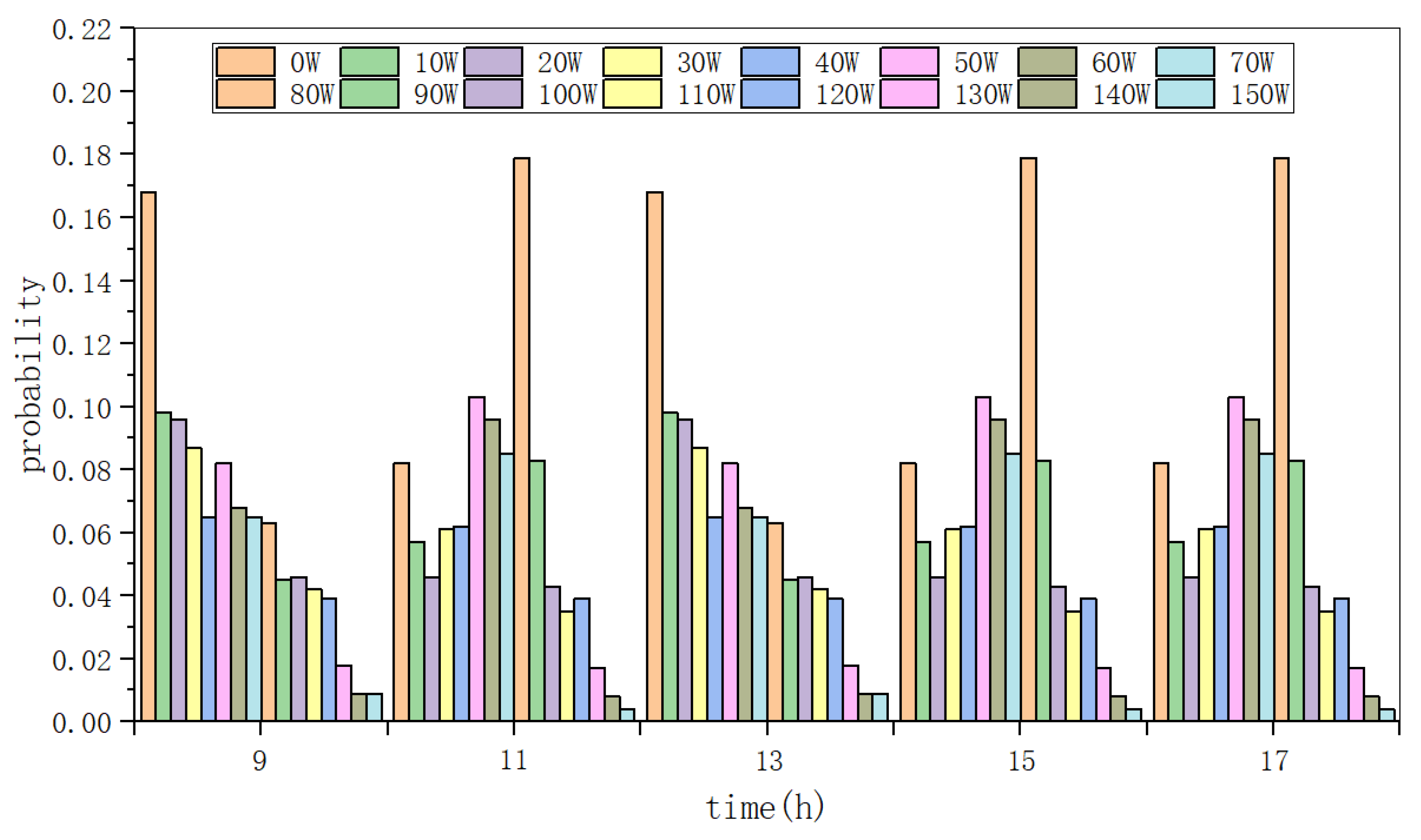
- Single-Use Appliances
- (iii)
- Communal Appliances
- (iv) Other Appliances
3. Model Validation and Analysis
3.1. Simulation Case Introduction
3.2. Simulation Results and Analysis
3.2.1. Determine the Number of Effective Electricity Users
3.2.2. Selection of Appliances
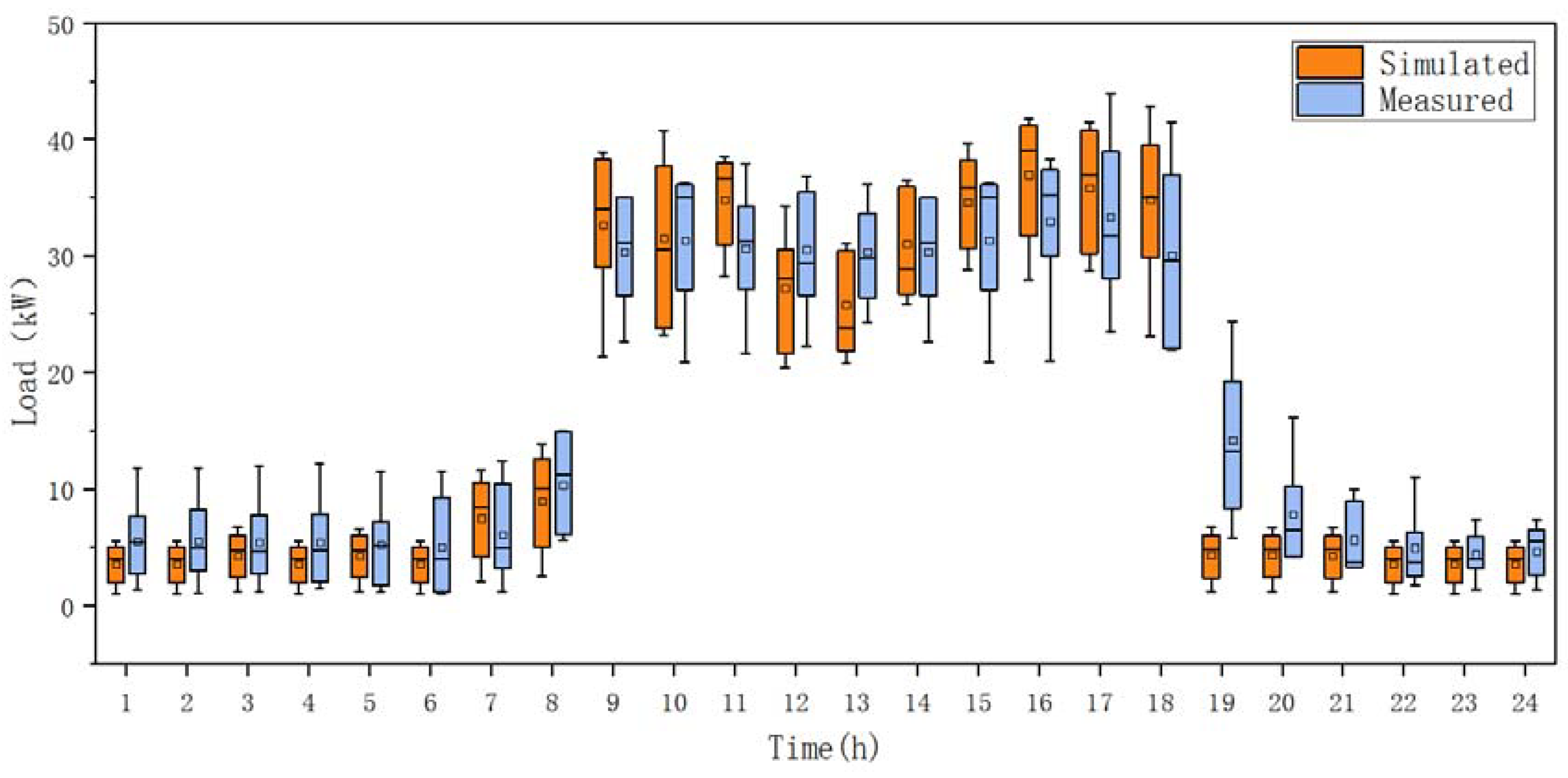
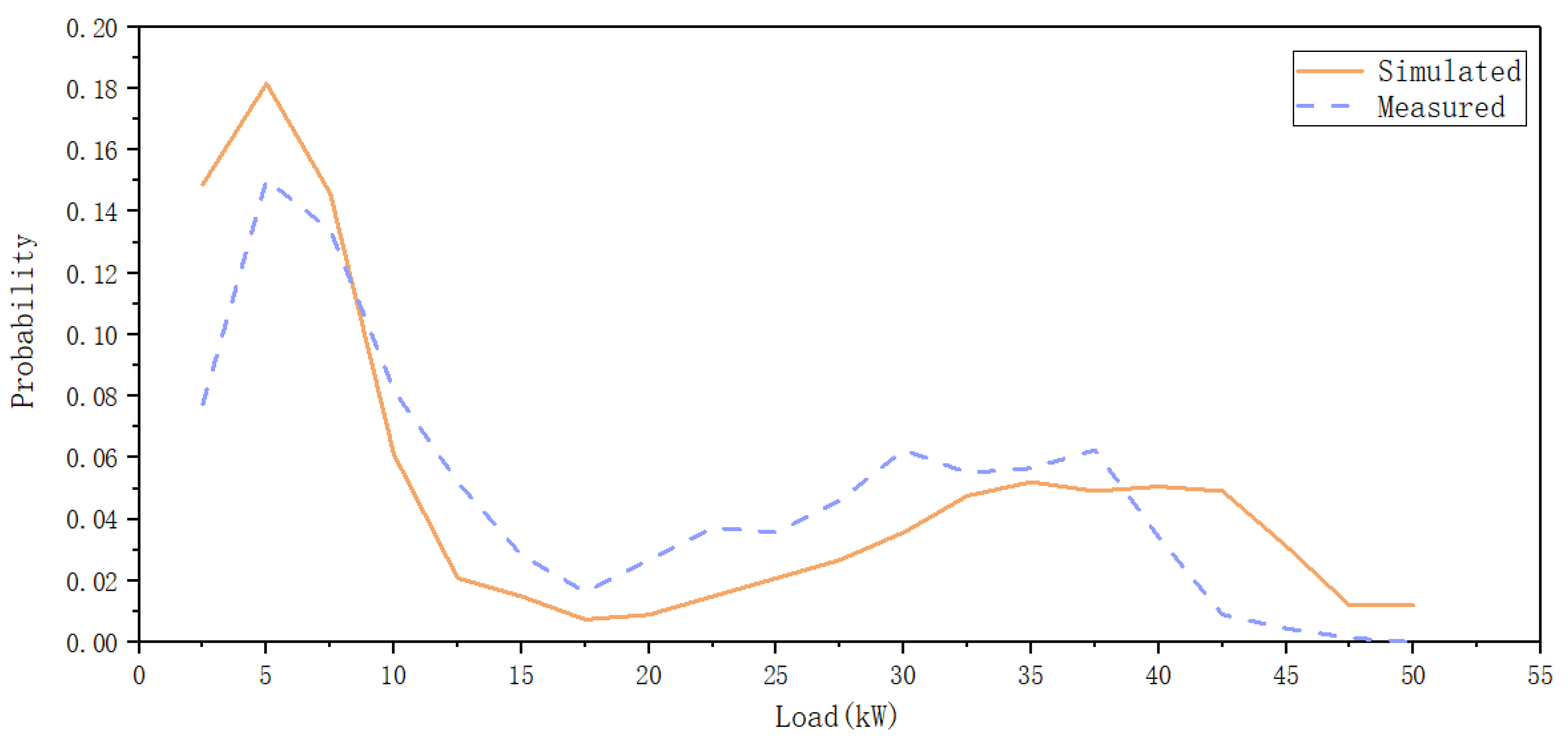
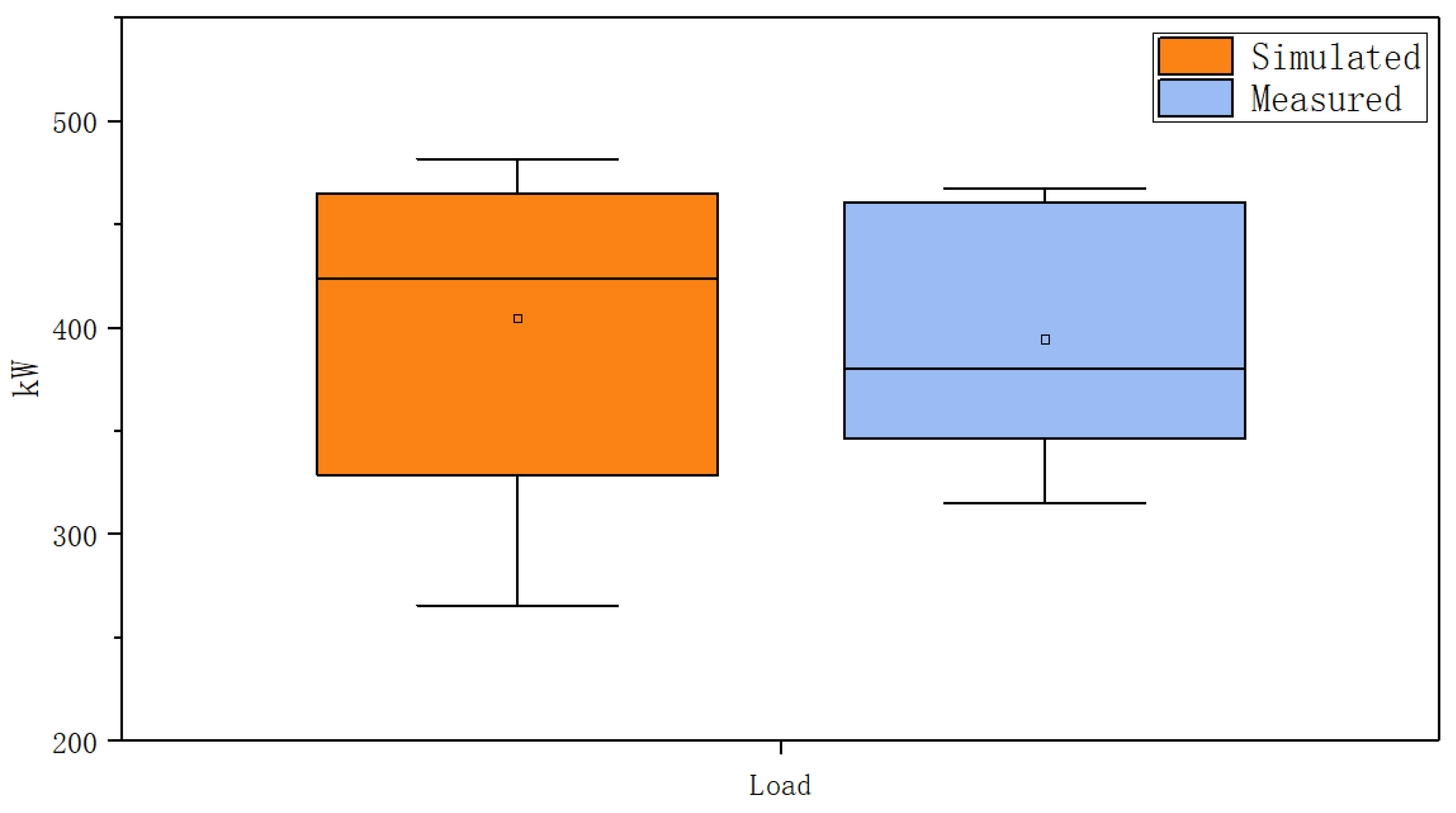
3.2.3. Simulation Results and Analysis
4. Discussion
5. Conclusions
Author Contributions
Funding
Acknowledgments
Conflicts of Interest
Abbreviations
| upper limits of solar radiation | |
| lower limits of solar radiation | |
| power of single-use appliance at kth level | |
| vertical solar radiation at time t | |
| K | power levels of single-use appliance |
| occupancy | |
| M | total number of office building |
| number of effective power users | |
| power of base appliances | |
| rated power of base appliances | |
| power of one single-use appliance | |
| power of single-use appliance | |
| probability of single-use appliance power at different levels | |
| per capita power density of office lighting | |
| power of appliance m | |
| standby power of appliance m | |
| used power of appliance m | |
| power of communal appliances | |
| power of elevator | |
| standby/used power of elevator | |
| power of office lighting | |
| P | power of office building |
| sharing coefficient of appliance m | |
| t | time |
| use probability of appliance m | |
| number of appliance m | |
| number of effective power users of appliance m | |
| r | random variables with uniform distribution on [0, 1] |
References
- Wang, Z.X.; Ding, Y.; Geng, G.; Zhu, N. Analysis of energy efficiency retrofit schemes for heating, ventilating and air-conditioning systems in existing office buildings based on the modified bin method. Energy Convers. Manag. 2014, 77, 233–242. [Google Scholar] [CrossRef]
- Fischer, D.; Hartl, A.; Wille-Haussmann, B. Model for electric load profiles with high time resolution for German households. Energy Build. 2015, 92, 170–179. [Google Scholar] [CrossRef]
- Zatti, M.; Gabba, M.; Freschini, M.; Rossi, M.; Gambarotta, A.; Morini, M.; Martelli, E. k-MILP: A novel clustering approach to select typical and extreme days for multi-energy systems design optimization. Energy 2019, 181, 1051–1063. [Google Scholar] [CrossRef]
- Voropai, N.; Stennikov, V.; Senderov, S.; Barakhtenko, E.; Voitov, O.; Ustinov, A. Modeling of integrated energy supply systems: Main principles, model, and applications. J. Energy Eng. 2017, 143, 04017011. [Google Scholar] [CrossRef]
- Min, D.; Ryu, J.H.; Choi, D.G. A long-term capacity expansion planning model for an electric power system integrating large-size renewable energy technologies. Comput. Oper. Res. 2018, 96, 244–255. [Google Scholar] [CrossRef]
- Liu, P.; Georgiadis, M.C.; Pistikopoulos, E.N. An energy systems engineering approach for the design and operation of microgrids in residential applications. Chem. Eng. Res. Des. 2013, 91, 2054–2069. [Google Scholar] [CrossRef]
- Wang, J.; Li, K.-J.; Liang, Y.; Javid, Z. Optimization of Multi-Energy Microgrid Operation in the Presence of PV, Heterogeneous Energy Storage and Integrated Demand Response. Appl. Sci. 2021, 11, 1005. [Google Scholar] [CrossRef]
- Wang, C.H.; Grozev, G.; Seo, S. Decomposition and statistical analysis for regional electricity demand forecasting. Energy 2012, 41, 313–325. [Google Scholar] [CrossRef]
- McLoughlin, F.; Duffy, A.; Conlon, M. Characterising domestic electricity consumption patterns by dwelling and occupant socio-economic variables: An Irish case study. Energy Build. 2012, 48, 240–248. [Google Scholar] [CrossRef] [Green Version]
- McLoughlin, F.; Duffy, A.; Conlon, M. Evaluation of time series techniques to characterise domestic electricity demand. Energy 2013, 50, 120–130. [Google Scholar] [CrossRef] [Green Version]
- Bucher, C.; Andersson, G. Generation of Domestic Load Profiles—An Adaptive Top-Down Approach. In Proceedings of the 12th International Conference on Probabilistic Methods Applied to Power Systems (PMAPS), Istanbul, Turkey, 10–14 June 2012. [Google Scholar]
- Gao, B.; Liu, X.; Zhu, Z. A Bottom-Up Model for Household Load Profile Based on the Consumption Behavior of Residents. Energies 2018, 11, 2112. [Google Scholar] [CrossRef] [Green Version]
- Hoverstad, B.A.; Tidemann, A.; Langseth, H.; Ozturk, P. Short-Term Load Forecasting with Seasonal Decomposition Using Evolution for Parameter Tuning. IEEE Trans. Smart Grid 2015, 6, 1904–1913. [Google Scholar] [CrossRef]
- Chuan, L.; Ukil, A. Modeling and Validation of Electrical Load Profiling in Residential Buildings in Singapore. IEEE Trans. Power Syst. 2014, 30, 2800–2809. [Google Scholar] [CrossRef] [Green Version]
- Hirst, E.; Lin, W.; Cope, J. Residential energy use model sensitive to demographic, economic, and technological factors. Q. Rev. Econ. Bus. 1977, 17. Available online: https://www.osti.gov/biblio/7088026-residential-energy-use-model-sensitive-demographic-economic-technological-factors (accessed on 1 November 2021).
- Bentzen, J.; Engsted, T. A revival of the autoregressive distributed lag model in estimating energy demand relationships. Energy 2001, 26, 45–55. [Google Scholar] [CrossRef]
- Moral-Carcedo, J.; Garcia, J.P. Integrating long-term economic scenarios into peak load forecasting: An application to Spain. Energy 2017, 140, 682–695. [Google Scholar] [CrossRef]
- Summerfield, A.J.; Lowe, R.J.; Oreszczyn, T. Two models for benchmarking UK domestic delivered energy. Build. Res. Inf. 2010, 38, 12–24. [Google Scholar] [CrossRef]
- Labandeira, X.; Labeaga, J.M.; Rodriguez, M. A residential energy demand system for Spain. Energy J. 2006, 27, 87–111. [Google Scholar] [CrossRef] [Green Version]
- Wenz, L.; Levermann, A.; Auffhammer, M. North–south polarization of European electricity consumption under future warming. Proc. Natl. Acad. Sci. USA 2017, 114, E7910–E7918. [Google Scholar] [CrossRef] [PubMed] [Green Version]
- Walker, C.F.; Pokoski, J.L. Residential Load Shape Modeling Based on Customer Behavior. IEEE Trans. Power Appar. Syst. 1985, 7, 1703–1711. [Google Scholar] [CrossRef]
- Widen, J.; Nilsson, A.M.; Wackelgard, E. A combined Markov-chain and bottom-up approach to modelling of domestic lighting demand. Energy Build. 2009, 41, 1001–1012. [Google Scholar] [CrossRef]
- Marszal-Pomianowska, A.; Heiselberg, P.; Larsen, O.K. Household electricity demand profiles—A high-resolution load model to facilitate modelling of energy flexible buildings. Energy 2016, 103, 487–501. [Google Scholar] [CrossRef]
- Jambagi, A.; Kramer, M.; Cheng, V. Residential electricity demand modelling: Activity based modelling for a model with high time and spatial resolution. In Proceedings of the IEEE 3rd International Renewable and Sustainable Energy Conference (IRSEC), Marrakech, Morocco, 10–13 December 2015. [Google Scholar]
- Sandels, C.; Widen, J.; Nordstrom, L. Forecasting household consumer electricity load profiles with a combined physical and behavioral approach. Appl. Energy 2014, 131, 267–278. [Google Scholar] [CrossRef]
- Sandels, C.; Broden, D.; Widen, J.; Nordstrom, L.; Andersson, E. Modeling office building consumer load with a combined physical and behavioral approach: Simulation and validation. Appl. Energy 2016, 162, 472–485. [Google Scholar] [CrossRef]
- Capasso, A.; Grattieri, W. A bottom-up approach to residential load modeling. IEEE Trans. Power Syst. 1994, 9, 957–964. [Google Scholar] [CrossRef]
- Paatero, J.V.; Lund, P.D. A model for generating household electricity load profiles. Int. J. Energy Res. 2006, 30, 273–290. [Google Scholar] [CrossRef] [Green Version]
- Foteinaki, K.; Li, R.L.; Rode, C.; Andersen, R.K. Modelling household electricity load profiles based on Danish time-use survey data. Energy Build. 2019, 202, 109355. [Google Scholar] [CrossRef]
- Nijhuis, M.; Gibescu, M.; Cobben, J.F.G. Bottom-up Markov Chain Monte Carlo approach for scenario based residential load modelling with publicly available data. Energy Build. 2016, 112, 121–129. [Google Scholar] [CrossRef] [Green Version]
- Vattenfall. Available online: http://corporate.vattenfall.com (accessed on 13 December 2015).
- Fischer, D.; Wolf, T.; Scherer, J.; Wille-Haussmann, B. A stochastic bottom-up model for space heating and domestic hot water load profiles for German households. Energy Build. 2016, 124, 120–128. [Google Scholar] [CrossRef]
- Fischer, D.; Stephen, B.; Flunk, A.; Kreifels, N.; Lindberg, K.B.; Wille-Haussmann, B.; Owens, E.H. Modeling the Effects of Variable Tariffs on Domestic Electric Load Profiles by Use of Occupant Behavior Submodels. IEEE Trans. Smart Grid 2016, 8, 2685–2693. [Google Scholar] [CrossRef] [Green Version]
- Wang, Z.X.; Ding, Y. An occupant-based energy consumption prediction model for office equipment. Energy Build. 2015, 109, 12–22. [Google Scholar] [CrossRef]


| Types of Appliances | Ownership Rate/% | Types of Appliances | Ownership Rate/% |
|---|---|---|---|
| printer | 90.8 | security monitoring | 93.2 |
| fax machine | 86.7 | water dispensers | 89.3 |
| scanner | 88.6 | network-related equipment | 99.6 |
| shredder | 67.8 | elevator | 99.3 |
| computer | 98.9 | projector | 90.1 |
| Parameters | Printer | Projector | Scanner | Computer |
|---|---|---|---|---|
| standby power/W | 10 | 10 | 10 | —— |
| working power/W | 360 | 480 | 400 | 0–150 |
| parameters | security monitoring | water dispenser | network-related equipment | elevator |
| standby power/W | 0 | 20 (warming) | 0 | 400 |
| working power/W | 24 | 120 (heating) | 36 | 1100 |
| Pmax | Pmin | Pava | |
|---|---|---|---|
| Simulated value/W | 49.04 | 3.87 | 15.08 |
| Measured value/W | 43.93 | 4.21 | 14.700 |
| Relative error/% | 11.63 | 8.08 | 2.04 |
| Regression Statistics | β | p-Value | R2 | RMSE |
|---|---|---|---|---|
| Simulated | 0.7073 | 0.001 | 89.29% | 1.558 |
| Measured |
Publisher’s Note: MDPI stays neutral with regard to jurisdictional claims in published maps and institutional affiliations. |
© 2021 by the authors. Licensee MDPI, Basel, Switzerland. This article is an open access article distributed under the terms and conditions of the Creative Commons Attribution (CC BY) license (https://creativecommons.org/licenses/by/4.0/).
Share and Cite
Cheng, S.; Tian, Z.; Wu, X.; Niu, J. Bottom-Up Model of Random Daily Electrical Load Curve for Office Building. Appl. Sci. 2021, 11, 10471. https://doi.org/10.3390/app112110471
Cheng S, Tian Z, Wu X, Niu J. Bottom-Up Model of Random Daily Electrical Load Curve for Office Building. Applied Sciences. 2021; 11(21):10471. https://doi.org/10.3390/app112110471
Chicago/Turabian StyleCheng, Sihan, Zhe Tian, Xia Wu, and Jide Niu. 2021. "Bottom-Up Model of Random Daily Electrical Load Curve for Office Building" Applied Sciences 11, no. 21: 10471. https://doi.org/10.3390/app112110471