Selecting Remote Driving Locations for Latency Sensitive Reliable Tele-Operation

Abstract

These days, autonomous vehicles (AVs) technology has been improved dramatically. However, even though the AVs require no human intervention in most situations, AVs may fail in certain situations. In such cases, it is desirable that humans can operate the vehicle manually to recover from a failure situation through remote driving. Furthermore, we believe that remote driving can enhance the current transportation system in various ways. In this paper, we consider a revolutionary transportation platform, where all the vehicles in an area are controlled by some remote controllers or drivers so that transportation can be performed in a more efficient way. For example, road capacity can be effectively utilized and fuel efficiency can be increased by centralized remote control. However, one of the biggest challenges in such remote driving is the communication latency between the remote driver and the vehicle. Thus, selecting appropriate locations of the remote drivers is very important to avoid any type of safety problem that might happen due to large communication latency. Furthermore, the selection should reflect the traffic situation created by multiple vehicles in an area. To tackle these challenges, in this paper, we propose several algorithms that select remote drivers’ locations for a given transportation schedules of multiple vehicles. We consider two objectives in this system and evaluate the performance of the proposed algorithms through simulations. The results show that the proposed algorithms perform better than some baseline algorithms.

1. Introduction

Recently, autonomous vehicles (AVs) technology has obtained a lot of attention, as it has significant effect on transportation systems. The technology that partially or totally replaces the driving task that was conducted by a human driver is referred as autonomous vehicle (AV) or self-driving vehicle. For the past several decades, various companies have been investing huge amount of resources into automated vehicles to make the best and most comfortable vehicles that are reliable and safe in every way.

The levels of AVs’ autonomy is divided into six stages by the Society of Automotive Engineers (SAE) [1,2]. The levels range from zero to five, from fully manual (level 0) to fully automated (level 5). However, until the autonomous technology becomes mature enough to be level 5, the experts suggest running the vehicles using tele-operations [3]. Remote driving is a mechanism in which a person controls a vehicle from a distance using communication networks. Actually, remote driving can overcome many situations where AVs may not be able to overcome. In other words, a human with advanced perceptual and cognitive skills could be added to the AV control loop via remote driving. This improves AVs’ dependability and efficacy [4]. People can trust remote driving because it has the ability to fill such a gap regarding safety.

There are some examples that show the feasibility of remote driving. Several automakers have teamed up with businesses and research institutes to create a car that can be controlled remotely. Furthermore, some of them have successfully driven a vehicle on real roads from a distance of hundreds of miles [5,6]. Even though remote driving can alleviate the problem of autonomous vehicles, latency is the biggest challenge for the safety of remote driving. Remote driving involves sending necessary data from the vehicle to a remote driver, who can then send control information to the remotely controlled vehicle. Thus, to drive a car safely from a distance, the information exchange should be done in a very short time. If the latency is large, the remote driving may also fail.

Additionally, regarding remote driving as a viable complementary measure to AV, we consider a revolutionary transportation platform, where all the vehicles in an area are controlled by some remote controllers or drivers so that transportation can be performed in a more efficient way. In such a remote control platform, we need to carefully choose the locations of remote drivers to reduce the latency between the remote drivers and the vehicles for the given transportation requests that consist of source-destination pairs of multiple vehicles. Intuitively, if we have more remote driving locations, the latency can be reduced. However, the cost of operating remote driving facilities may increase. Thus, there are some trade-offs between the latency and the number of remote driving locations.

In this paper, we first define two objectives in selecting remote driving locations considering various requirements and constraints. The two objectives reflect two different situations in selecting remote driving locations. First one is to select the driving locations in such a way that we want to keep the number of selected location low as long as the selected locations satisfy the given latency constraint. The latency constraint represents the upper bound of the latency between the remote drivers and the vehicles. By reducing the number of driving locations, we can reduce the operating costs. The second one is to reduce the latency as much as possible while selecting a fixed number of driving locations. In this objective, the operation cost is fixed because the number of driving locations is fixed. Thus, with the same amount of cost, we want to increase the safety of remote driving by reducing the latency between the drivers and the vehicles. We then propose several algorithms to achieve the two objectives and evaluate the performance of the algorithms. We compare the proposed algorithms with some baseline algorithms and two preliminary algorithms proposed in [7,8], respectively. The contributions of the paper can be summarized as follows.

• We formally define two objectives in a more concrete way.
• We propose heuristic algorithms to achieve the two objectives.
• We evaluate the proposed heuristic algorithms through extensive simulations.

The rest of the paper is organized as follows. Section 2 provides background and literature reviews about AVs and remote driving. We describe the problem statement and propose algorithms for the two objectives in Section 3. Evaluation results are given in Section 4. Section 5 concludes the paper.

2. Background and Literature Review

In this section, we briefly discuss the historical perspectives, related works, and issues with remote driving systems. In a remote driving environment, a driver controls a vehicle through tele-operation. In order to control a vehicle in real time, real-time data transmission is needed, which exploits today’s networking infrastructure. Latency is a crucial factor for secure and reliable driving. In the following, we describe many related works showing the feasibility of remote driving under the current communication infrastructures such as LTE and Wi-Fi.

A truly autonomous vehicle was first suggested by S. Tsugawa at Japan Tsukuba Mechanical Engineering Laboratory [9]. The vision of “future highway” for autonomous vehicles has been proposed back in 1960 to 1975 by Radio Corporation of America (RCA) [10]. Because of the remarkable benefits, local governments and several automobile manufacturers have invested in growing self-driving automobiles since 1977. These days, autonomous vehicles have mature hardware capabilities to allow absolute self-driving, but the driving emphalgorithms are still immature. In Figure 1, the adoption timeline for autonomous vehicles has been given [9]. A luxury automobile has approximately a hundred million lines of software program code, whilst the RF-22 Raptor fighter aircraft has 1.7 million [11]. In what are known as “disengagement reports”, self-driving cars with large base software code have been confirmed to have 2578 failures. These findings have been compiled by using nine corporations that carried out self-driving car avenue checks in 2016 [12].

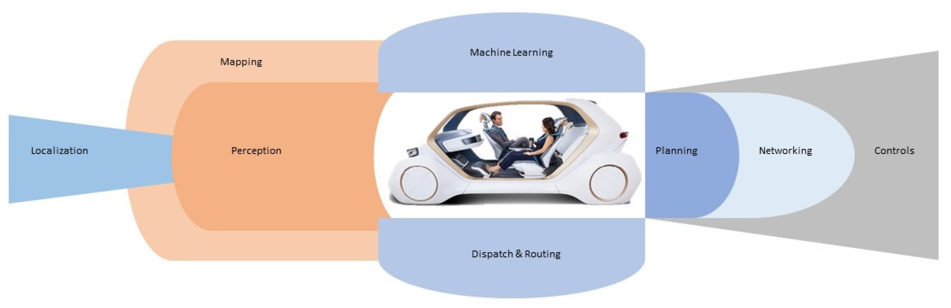
A variety of cutting-edge technologies are needed to ensure that everything works together smoothly such as localization, mapping, perception, machine learning, planning, networking, dispatch and routing, and controls [8,14]. In other words, these features are needed to recognize the world around the car and make decisions for the better driving. We summarize these features in Figure 2. As can be clearly seen in Figure 2, software is at the heart of the self-driving abilities. However, software inevitably contains bugs.

To overcome the problems caused by the software bugs, researchers explore special strategies to involve human beings within the control loop to manipulate diverse gadgets until the software in autonomous cars is sufficiently capable of preventing fatal failures. One example of such fatal failures is the crash happened on a divided toll road with a horizontal line [15]. According to the official accident report, cameras and radar are used by the autopilot to track and avoid obstacles, and the cameras were unable to discern “the white side of the tractor trailer against a brightly lit sky”. The radar should have detected the trailer without issue, but, according to Musk, “radar tunes out what appears to be an overhead road sign to stop false braking events”.

Remote driving can be implemented through high speed communication networks. Huawei, China Mobile, and SAIC Motor have demonstrated 5G-based vehicles. In a remote driving test, the driver was 30 km away from the automobile and the latency for control functions was 10 ms [6]. Telefonica and Ericsson also confirm remote driving as a reality, where they ensure the reliability of driving a car located 70 km away through 4K videos using sensory perception [16].

The researchers have peered into the future of tele-operated devices, examining device architecture while considering network delay as a primary constraint. A previous research found that the major factor that affects remote driving efficiency is the magnitude and the variability of the feedback [17]. A delay of 170 ms has been found a minor impact on remote driving efficiency [18]. As the delay reaches 700 ms, driving performance suffers significantly. A commercial long term evaluation (LTE) network has been used to investigate human behaviors in remote driving, where they use a scaled remote driving prototype and conduct a controlled human study with different network delays [19]. They conclude that performance degradation is caused by network delay variability rather than magnitude. Furthermore, they conclude that the current LTE network is infeasible for remote driving. However, in another study, a real-time streaming testbed for a vehicular environment through audio visual techniques has been evaluated on frame latency under several parameter settings with today’s LTE and Wi-Fi networks [3]. The results show that the median latencies of LTE and Wi-Fi are around 100 ms and 50 ms, respectively, which may be acceptable for remote driving. In [20], a model car has been tested for remote and virtual driving by using Wi-Fi, and the experimental results confirm the reliability in real-time remote driving.

In [5], a static multi-camera with fusion display and 3G communication network has been used for remote driving of vehicles to guarantee the safety of driving. A lightweight passive tool has been introduced for the identification of present LTE networks flaw (“used bandwidth less than 50 percent of the available bandwidth”). They suggest a remote control mechanism by using a more LTE friendly transport protocol and applications [21]. In [22], LTE-Advanced features have been highlighted to improve the quality of service (QoS) specifically focusing on network capacity delivery in terms of offloading and congestion control. Refs. [19,23] broadly investigate those factors that influence human remote driving. Refs. [17,19] reveal that when delay exceeds 700 ms, driving performances significantly degrade and delay beyond 1 s restricts the effective real-time interactions through tele-operation. Ref. [18] also finds that the efficiency of human remote driving is influenced by small constant delays. Actually, ref [19] shows that a local Internet with distance around 1000 mile can provide a round trip time RTT of 16 ms with 4 Mbps minimum bandwidth. Thus, the current communication network is sufficient enough to support the remote driving technology. In our paper, remote drivers actually control and monitor the vehicles. Similarly, even though an autonomous vehicle can operate by itself, someone need to monitor the vehicles for various purposes. For the remote monitoring, a large amount of data should be transmitted from the vehicle to the operation center. Ref. [24] proposes a compression method of LIDAR data specifically. Since the data set is a time series data, they apply various signal processing methods such as discrete cosine transform (DCT) and differential sampling. This method can be also used in remote driving systems for efficient transmission of the sensor data.

Autonomous driving may have many security attacks. Ref. [25] provides a list of attack or security threat mechanisms and proposes counter measures of those problems. Specifically, they focus on localization and navigation technologies. Those issues should be addressed in any autonomous driving systems. There can be various algorithms for autonomous driving. Thus, it is necessary to evaluate those algorithms in a standard platform. Ref. [26] proposes an evaluation platform that jointly considers vehicular communication, road traffic and vehicle dynamics. They combine many existing simulators such as SUMO and CARLA to simulate various road and traffic situations. Furthermore, they investigate the behavior of a remote driving application based on CARLA. This platform may be useful for testing any new algorithms and applications. In remote driving, the network infrastructure between the driving center and the vehicle is crucial for the safety of the driving. Ref. [27] investigates the key features of 5G NR-V2X technologies. Furthermore, they discusses the evolution of the V2X (vehicle-to-everything) technologies to provide better understanding of the communication infrastructure. Since the infrastructure is evolving continuously, the remote driving is likely to become a reality in the near future. Actually, ref [28] investigates whether tele-operated driving is possible with contemporary mobile networks. Their results show that the high variance of the network parameters influences the performance of remote driving. This result clearly indicates that better network infrastructure is needed for safe remote driving.

In autonomous driving, AI plays an important role. However, the computation requirement of AI is quite large, so where the computation should be done is very important. Ref. [29] discusses the autonomous driving Cognitive Internet of Vehicles. To be specific, they focus on what to compute, where to compute, and how to compute for the AI of the autonomous vehicles. Since the remote driving can evolve to a remote driving by AI, the suggestions of this paper that considers the computation and communication together can be applicable to our proposed system, too. Each task of the autonomous driving may require a specific algorithm. For example, ref [30] presents a lane changing algorithm by using deep deterministic policy gradient learning algorithm. This algorithm is run at the vehicle. So depending on the specific task, where to compute should be determined.

Actually, the two objectives of this paper are similar to clustering problems or node placement problems in wireless networks [31,32,33]. For example, ref [34] tries to deploy access points in an area to cover as many wireless mesh clients as possible. In this paper, we try to select the locations of remote driving facilities given the locations of base stations. However, in this paper, we only consider the base stations along the routes of the vehicles. Thus, we exploit this specific characteristics of remote driving to achieve better performance rather than just applying other general clustering algorithms or node placement algorithms.

To date, we have discussed a number of existing works related to remote and autonomous driving. We summarize the above technologies by categorizing them depending on the research area in

Table 1. Summary of existing technologies.

Research Area	Main Research Issues
Autonomous Driving Concepts and Components	Autonomous driving needs many software components such as Localization, Mapping, Perception, Machine Learning, Dispatch & Routing, Planning, Networking, and Controls [9,10,14].
Communication	Autonomous vehicles and remote driving vehicles need to exchange information between controlling center and the vehicle for monitoring and controlling purposes. Thus, the communication infrastructure is very crucial in the success of autonomous and remote driving [3,16,17,19,20,27,28].
Sensors	Remote driving vehicles have many sensors such as camera and LIDAR. The sensor information should be transmitted to the monitoring center and the delay should be within some delay bound. The relationship between the delay and the driving performance has been investigated a lot [17,19,21,22,23,24].
Security	Since autonomous driving and remote driving may cause serious accidents due to many reasons, the security of those technology should be considered with the highest priority. Researches regarding security of autonomous and remote driving have been studied a lot [25].
Computation	Algorithms needed for autonomous and remote driving may require high computation time. Since the computation capacity of a vehicle may be limited, it is necessary to have additional computation power from elsewhere. How to distribute the computation job to various places can be a good research issue [26,29,30].
Node Placement Algorithms	Identifying driving location problem is similar to clustering problem given a number of points in a 2 or 3 dimensional area. The objectives can be reducing the average distance from the cluster centers or increasing signal strength in a wireless networks [31,32,33,34].

. These technologies deal with various aspect of autonomous and remote driving. However, in this paper, we focus on remote driving location selection problem, which is not addressed by the related works.

3. Selecting Driving Locations for Multiple Paths

In this paper, we consider a revolutionary transportation system, where a logically centralized remote controller controls all the vehicles in an area. A driving location is a place where the remote controller or a driver controls a vehicle through communication networks. To start the discussion, let us consider a simple case with one vehicle. The vehicle has a route from an origin to a destination. A route in the real world is a sequence of road segments. For a remote driver to control the vehicle, the driver needs to communication with the vehicle through the communication network infrastructure. Since the vehicle is mobile, the edge of the communication network should be a base station, which has a direct wireless link to the vehicle. So there must be a sequence of such base stations from the origin to the destination along the route. Since we focus on the remote driving technology, we only need to consider the sequence of base stations instead of the real route of roads itself.

Thus, we consider a sequence of base stations as a route in this remote driving system. Actually, we assume that if the origin and the destination of a route are given, the sequence of base stations is easily obtained. In other words, the route of a vehicle can be easily represented by the sequence of base stations along the path. Thus, we assume that a vehicle to infrastructure communication, V2I, is established between a remote driver and the vehicle through base stations along the paths. As the vehicle moves toward the destination, the communication to the vehicle is transferred to the next base station along the path. Figure 3 shows two routes, each of which consists of a sequence of base stations. For example, the vehicle of “Path 1” may start the communication with $B_7$, then it is reconnected to $B_8$, and so on.

If a driver in a location, for example $d_1$, controls the vehicle from the start to the end, the latency between $d_1$ and $B_{11}$, the final base station, is likely to be very large so that the performance of remote control may degrade and even cause accidents. Thus, it is necessary for different drivers in different driving locations to control the vehicle for different segments of the paths to satisfy the safety requirement such as a latency limit. Since we cannot deploy the drivers to every base station in the area due to the management cost, we need to select a set of driving locations in the area in such a way that the selected locations satisfy the requirement of the remote driving system.

In this paper, we extend the single path case to the multiple path case and select the driving locations for multiple paths. For this problem, we assume that the sequence of base stations of the multiple paths are given. The requirement of the remote controlling system may differ depending on many factors such as management cost and latency limit. Thus, we consider the following two objectives, which are likely to incorporate various requirements of different remote driving systems.

• Objective I: Selecting the smallest number of driving locations while satisfying a given latency threshold.
• Objective II: Selecting a set of driving locations that minimize the latency between the vehicles and driving locations when the number of driving locations is fixed.

In the first objective, we assume that the remote driving is safe if the latency is under a certain threshold. Under this assumption, we want to minimize the number of remote driving locations to reduce the management cost. Furthermore, if there are multiple sets of driving locations of same size that satisfy the latency constraint, we may want to choose the set of driving locations that has the smallest latency. In the second objective, the number of driving locations is fixed, which means that the cost of maintaining the driving locations is fixed. With the given budget of driving locations, we want to reduce the latency as much as possible. It should be noted that depending on various situations, the latency constraint or the number of driving locations may vary.

Actually, in [7], we have proposed an algorithm called “Remote driver Selection for Multiple Paths (RDSMP)”, which selects the driving locations when a latency threshold is given. Basically RDSMP focuses on the objective I. However, RDSMP does not consider the latency further when it finds a certain number of driving locations. To be specific, there can be different sets of the same number of driving locations that satisfy the latency constraints. Then, we might want to have a set of driving locations that can reduce the latency as much as possible. In other words, even though the selected driving locations satisfy the latency constraints, it would be better to reduce the latency as much as possible by selecting other sets of driving locations of the same size.

Furthermore, in this paper, we newly formulate Objective II on top of Objective I to deal with many other situations. Thus, in this paper, we propose a comprehensive set of algorithms for the above two objectives. For all the algorithms, we assume that the candidate driving locations are given instead of assuming that any location in the area can be a driving location. It is quite reasonable to assume the candidate locations because we might not be able to build a remote driving facility in any location due to many reasons such as rental costs, geographic constraints, and communication infrastructure. Basically, we choose the driving locations from the candidate set.

Before we describe the algorithms in detail, we first define some notations at

Table 2. Notations.

Notation	Definition
$\mathcal{F}$	$\{d_1,d_2,\dots ,d_m\}$, the set of candidate driving locations. Thus, there are m candidate locations, from which we select a set of driving locations.
$\mathcal{B}$	$\{B_1,B_2,\dots ,B_n\}$, the set of base stations in the area. Thus, there are n base stations in the area.
P	$\{P_1,P_2,\cdots ,P_l\}$, the set of paths given to the algorithms. Thus, there are l paths.
$dist(d,b)$	the distance (or latency) between a driving location $d\in \mathcal{F}$ and a base station $b\in \mathcal{B}$. The distance is the network distance. We use distance and latency interchangeably.

. Furthermore, we use the term “driving location” and a “driver” interchangeably because selecting a driving location means selecting a driver in that location.

3.1. Selecting the Smallest Number of Remote Drivers under Latency Constraint

In this subsection, we propose an algorithm called Extended Remote Driver Selection for Multiple Paths (ERDSMP) for Objective I. Actually, ERDSMP tries to improve the performance of RDSMP of [7]. Let L be the latency constraint, which is the largest allowable latency between a remote driving location and the vehicle. If the latency is larger than L, the safety of the remote driving degrades. We try to find a smallest set of driving locations (or simply drivers) that satisfy the latency constraint. Furthermore we want to minimize the average latency between the selected driving locations and the sequence of the base stations of the path. Since at every moment, the distance between a driver and the vehicle should be within L, we define the distance between a selected set of driving locations, $D\subseteq \mathcal{F}$, and the set of base stations, $B\subseteq \mathcal{B}$ in Equation (1).

$$\begin{array}{cc}\hfill Dis{t}_{max}(D,B)& =\underset{b\in B}{\max }\left(\underset{d\in D}{min}dist(d,b)\right)\hfill \end{array}$$

(1)

Thus, the algorithms for Objective I are to solve the following optimization problem. In other words, the longest distance between D and B, the set of base stations for the given paths P, should be less than or equal to L. By this way, the safety of the remote control system is obtained.

$$\begin{array}{cc}\hfill \mathrm{minimize}& \left|D\right|\hfill \\ \hfill \mathrm{such}\mathrm{that}& D\subseteq \mathcal{F}\hfill \\ \hfill & Dis{t}_{max}(D,B)\le L\hfill \end{array}$$

(2)

Now, we describe ERDSMP in detail. ERDSMP actually uses RDSMP in it. So, we briefly describe RDSMP [7]. As we define before, there are l origin-destination pairs in P. $P_i$ is the ith path, which has a sequence of base stations $(B_{i_1},B_{i_2},\dots ,B_{i_{l_i}})$ of length $l_i$. The objective of RDSMP is to find a reasonably small set of driving locations $D\subseteq \mathcal{F}$ that can cover all the base stations in P. The first step of RDSMP is to reduce the search space by filtering out the driving locations that are not within the latency of L from any of the base stations in P. It is clear that those driving locations cannot be used to cover any of the base stations. Let C be the remaining driving locations, which are the reduced set of candidate driving locations.

For each driving location in C, we compute how many base stations that the driving location can cover under the given latency constraint. For example, if a driving location d covers 2 base stations in $P_1$, 3 base stations in $P_2$, and 4 base stations in $P_4$, we consider that d covers $9(=2+3+4)$ base stations. Furthermore, when doing this counting, we only count the consecutive base stations from each “end” of the paths in P. In other words, even though a driving location covers 10 base stations in the “middle” of a path, we consider that the driving location covers 0 base stations because it does not cover any base station at the two ends of the path. The reason is because we do not want to break the sequence of base stations into many pieces. For example, consider a path with 100 base stations. Suppose that a driving location covers 98 base stations in the “middle”. If we choose the driving location because it covers the most base stations, then the path is broken into three pieces. So we need two more driving locations to cover each “end” of the path. Thus, we need three driving locations to cover the entire path. However, if there are two driving locations that can cover the first 50 base stations and the last 50 base stations, respectively, then we only need two driving locations. In short, we count the covered base stations from the ends of the paths. After we select the driving location that covers the most base stations, we add the driving location into the solution set, D. Then, we remove the base stations that are covered by the driving location, which results in shortened paths in P. We repeat this process until we do not have any path that is not covered by D. The details can be found in Algorithm 1.

ERDSMP is a simple extension of RDSMP. The purpose of ERDSMP is to choose a set of driving locations, of which the size is the same as that of RDSMP, but the average distance between the selected driving locations and the base stations is lower than that of RDSMP. The definition of the average distance between a driving location set $D\subseteq \mathcal{F}$ and the set of base stations $B\subseteq \mathcal{B}$ is as follows.

$$\begin{array}{cc}\hfill Dis{t}_{avg}(D,B)& =\frac{1}{\left|B\right|}\sum _{b\in B}\left(\underset{d\in D}{min}dist(d,b)\right)\hfill \end{array}$$

(3)

In short, we want to find a driving location set D that solves the problem of (2) and has as small a value of $Dis{t}_{avg}(D,B)$ as possible. For that matter, ERDSMP slightly modifies RDSMP. Basically, RDSMP is a simple greedy algorithm, in which we choose the first driving location that covers the most base stations. However, other choices of the first selected driving location may provide a better result. Thus, we first find a set of driving locations, I, that cover the base stations from each ends of the paths just like RDSMP. Then, instead of choosing the driving location that covers the most base stations, we just take each driving location from I, then run RDSMP from that on. This procedure provides $\left|I\right|$ different sets of driving locations. Among them, we choose the set of driving locations that has the smallest average distance between the driving locations and the base stations.

As an example, consider Figure 3. In Figure 3, RDSMP chooses D = $\{d_2,d_3,d_5\}$. However, $d_1$ also covers $B_1$. Actually, $I=\{d_1,d_2,d_5\}$ are the set of driving locations that cover the first base stations of the two paths from both ends. So in ERDSMP, we take each I as the first selected driving location and run RDSMP for the remaining paths base stations. This gives another feasible set of driving locations, $D^{\prime }$= $\{d_1,d_3,d_5\}$, which have $d_1$ as a firstly selected driving location. Since $D^{\prime }$ has the smaller average distance than D, ERDSMP chooses $D^{\prime }$. Basically, $D^{\prime }$ reduces the average distance compared to D. It is clear that the average distance of $D^{\prime }$ is always equal or less than that of D. The description of ERDSMP is given in Algorithm 2.

Algorithm 1 RDSMP.

1: Input: ($P,\mathcal{F},L$)  2: Output: D  3: P: Src-Dst Path List  4: $\mathcal{F}$: Set of candidate driving locations  5: L: Latency Threshold  6: D: Solution Set  7: $B\leftarrow$ all the base stations in P  8: $C\leftarrow Ø$  9: for $d\in \mathcal{F}$ do 10:  if there is any base station, $b\in B$, such that $dist(d,b)\le L$ then 11:   $C\leftarrow C\cup \left\{d\right\}$ 12: $D\leftarrow Ø$ 13: while P is not empty do 14:  for $d\in C$ do 15:   $S\left(d\right)\leftarrow$ the set of base stations in P that d covers 16:  $d\leftarrow \underset{d\in C}{arg\; max}\left|S\right(d\left)\right|$ 17:  Shorten the paths in P by removing the base stations in $S\left(d\right)$ 18:  $D\leftarrow D\cup \left\{d\right\}$ 19:  $C\leftarrow C-\left\{d\right\}$ 20: return D

Algorithm 2 ERDSMP.

1: Input: ($P,\mathcal{F},L$)  2: Output: D  3: P: Src-Dst Path List  4: $\mathcal{F}$: Set of candidate driving locations  5: L: Latency Threshold  6: D: Solution Set  7: $B\leftarrow$ all the base stations in P  8: $C\leftarrow Ø$  9: for $d\in \mathcal{F}$ do 10:  if there is any base station, $b\in B$, such that $dist(d,b)\le L$ then 11:   $C\leftarrow C\cup \left\{d\right\}$ 12: $D\leftarrow$ RDSMP $(P,C,L)$ 13: $ad\leftarrow$$Dis{t}_{avg}(D,B)$ 14: $E\leftarrow$ the set of driving locations which cover at least one first base stations of P 15: for $d\in E$ do 16:  Let G be the set of the base stations along the paths, P, that d covers 17:  $P^{\prime }\leftarrow$ Shortened paths in P by removing the base stations in G from P 18:  $D^{\prime }\leftarrow RDSMP(P^{\prime },C,L)$ 19:  if $\left(\right(|D^{\prime }|==|D\left|\right)\wedge (ad>Dis{t}_{avg}(D^{\prime },B))$ then 20:   $ad\leftarrow Dis{t}_{avg}(D^{\prime },G)$ 21:   $D\leftarrow D^{\prime }$ 22: return D

3.2. Selecting a Fixed Number of Driving Locations for Smallest Distance

Now, let us turn our focus to Objective II. As we have seen earlier, in Objective II, the size of the driving locations is fixed to a certain constant. Thus, if we want to choose k driving locations from the candidate driving location set $\mathcal{F}$, there are $\left(\genfrac{}{}{0pt}{}{\left|\mathcal{F}\right|}{k}\right)$ different sets of k driving locations. In Objective II, we want to select the driving location set D that has the smallest distance to the base station set B of P. Thus, the algorithms for Objective II try to find a set of k driving locations, D, that minimizes the $Dis{t}_{max}(D,B)$. In other words,

$$\begin{array}{c}\hfill D=\underset{D\in \mathcal{P}(\mathcal{F},k)}{\mathrm{argmin}}Dis{t}_{max}(D,B)\end{array}$$

(4)

where $\mathcal{P}(\mathcal{F},k)$ is the set of all possible subsets that has k members of $\mathcal{F}$. However, finding the best set may not be feasible since $\left(\genfrac{}{}{0pt}{}{\left|\mathcal{F}\right|}{k}\right)$ is very large. Instead, we propose two heuristic algorithms that find an approximate solution of Equation (4). In short, we want to have a set D that has as small value of $Dis{t}_{max}(D,B)$ of Equation (1) as possible.

Before we propose heuristic algorithms, we first describe a baseline algorithm called “Random Search”. In “Random Search”, we randomly select a driving location set D from $\mathcal{P}(\mathcal{F},k)$. Then, we compute $Dis{t}_{max}(D,B)$. We repeat this procedure for a certain number of iterations and choose the driving location set, D, that gives the smallest distance $Dis{t}_{max}(D,B)$ so far. Intuitively, if we increase the number of iterations of “Random Search”, the result becomes better.

Now we propose two heuristic algorithms, which are based on binary search and k-means algorithms, respectively. The first heuristic algorithm is called “BS”, which exploits ERDSMP. Since ERDSMP finds a small set of drivers for the given latency constraint L, we systematically try different values of L for ERDSMP and find the set of driving locations corresponding to L. If we can find a smallest L for which ERDSMP generates exactly k driving locations, the resulting set of k driving locations is the solution of the objective II. One way to do this is to check L sequentially. So we just start from a very small L and run ERDSMP. We repeat this procedure by increasing L slightly. When L is small, the resulting set of ERDSMP may contain a large number of driving locations. However, if we increase L, then the size of the resulting set of ERDSMP decreases. When the size of the resulting set of ERDSMP is k, we can stop. However, this kind of sequential search may take very long time. Since the problem is just a simple search problem, instead of using sequential search, we use a binary search method to search the smallest L for which ERDSMP find k driving locations. The details are shown in Algorithm 3. One thing to note is that since L is a real number, we cannot search all the possible values of L. Instead, we search the values of L in the granularity of $\delta$, which is a very small value, for example, 0.1 unit of the distances.

Now, we describe another heuristic algorithm called “K-Means”, which is based on k-means clustering algorithm [35]. Since we want to select k driving locations that can cover a set of base stations and we want the distance as small as possible, we apply k-means algorithm over the set of base stations B of P. This provides the centroids of k clusters. However, the centroids may not coincide with the candidate driving locations $\mathcal{F}$. Thus, we choose the closest driving location to each centroid, which finds k driving locations from $\mathcal{F}$. Since the algorithm is as simple as it is, we do not elaborate further.

Algorithm 3 BS.

1: Input: $(P,\mathcal{F},k)$  2: Output: D  3: P: List of src-dst paths  4: $\mathcal{F}$: set of candidate driving locations  5: k: given number of drivers  6: D: Solution Set  7: $lb\leftarrow \delta$ // the smallest distance, lower bound  8: $ub\leftarrow$ the largest distance in the area // upper bound  9: while $lb<ub$ do 10:  $L\leftarrow \frac{lb+ub}{2}$ 11:  $H\leftarrow ERDSMP(P,\mathcal{F},L)$ 12:  if $\left|H\right|>k$ or H is empty then 13:   $lb\leftarrow L+\delta$ 14:  else if $\left|H\right|=k$ then 15:   $ub\leftarrow L-\delta$ 16:   $D\leftarrow H$ 17:  else 18:   $ub\leftarrow L$ 19: returnD

Actually, as we have seen in Equation (4), this problem is an optimization problem, in which the constraint is k, and we try to minimize the distance. Thus, general optimization algorithms such as simulated annealing and genetic algorithm may work for this problem. In this paper, we use simulated annealing as another baseline algorithm to evaluate the performance of the previous two heuristic algorithms. In reality, it might not be feasible to use simulated annealing due to large time complexity. We use simulated annealing to check whether the proposed heuristic algorithms perform near optimal.

Since simulated annealing is a well known algorithm, we just briefly mention some necessary information specific to our problem. For simulated annealing, we first find an initial subset of k driving locations, H, and measure its distance to the base stations, B of P. H becomes the current solution. Then, we choose a neighbor solution, $H^{\prime }$, which is a solution slightly different from H. In our implementation, we just randomly choose a driving location in H and replace it by another randomly selected driving location from $\mathcal{F}$. Then, we compute the distance from $H^{\prime }$ to B. Based on the distances from H and $H^{\prime }$, we compute the transition probability to the neighbor solution. Based on that transition probability, we may move to the neighbor solution or stay at the current solution. We repeat this process for a predefined number of iterations. The detail is shown in Algorithm 4.

Algorithm 4 SA.

1: Input: ($P,\mathcal{F},k,r$)  2: Output: D  3: P: List of src-dst paths  4: $\mathcal{F}$: set of candidate driving locations  5: k: given number of drivers  6: r: number of iterations  7: D: Solution Set  8: // initialization  9: $B\leftarrow$ set of base stations in P 10: $H\leftarrow$ randomly selected k driving locations from $\mathcal{F}$ 11: $f_1\leftarrow Dis{t}_{max}(H,B)$ 12: $T\leftarrow 10,000$ 13: $\alpha \leftarrow {\left(\frac{0.0001}{T}\right)}^{\frac{1}{r}}$ 14: for $i=1$ to r do 15:  $H^{\prime }\leftarrow$ a randomly selected neighbor of H 16:  $f_2\leftarrow$$Dis{t}_{max}(H^{\prime },B)$ 17:  $p\leftarrow exp\left(\frac{f_1-f_2}{T}\right)$ 18:  $p^{\prime }\leftarrow$ a random number in $(0,1)$ 19:  if $p^{\prime }<p$ then 20:   $H\leftarrow H^{\prime }$ 21:   $f_1\leftarrow f_2$ 22:  if $f_1>f_2$ then 23:   $D\leftarrow H^{\prime }$ 24:  $T\leftarrow T\times \alpha$ 25: returnD

4. Evaluation

In this section, we evaluate the performance of remote driving location selection algorithms proposed in the previous section. For the evaluation, we assume a transportation environment of 3000 base stations, i.e., $\left|\mathcal{B}\right|=3000$ and 500 candidate remote driving locations, i.e., $\left|\mathcal{F}\right|=500$, in the area of 1000 × 1000, where base stations and remote driver are uniformly randomly distributed over the entire area. One thing to note is that we do not specify the unit of the area and the latency constraints L because the main purpose of this paper is to propose algorithms for various situations. Thus, depending on situations, the unit could be meters or kilometers and so on. The number of origin-destination pairs is 1000, i.e., $\left|P\right|=1000$. One subtle thing is the unit of the latency constraint L. We need to provide a time unit for the latency constraint. However, since the latency is proportional to the distance, we specify the latency constraint L in terms of distance. For example, latency constraint 300 means 300 distance unit.

Actually, the origin and destinations are simply base stations that are uniformly randomly selected from $\mathcal{B}$. Then, we need to find the sequence of base stations between the origin and the destination. Since we do not have any road map on this synthetic data set, we mimic the road map by using Delaunay triangulation [36]. To be specific, we run Delaunay triangulation with the positions of the base stations. This generates a planar graph with base stations as nodes. The edges constructed from the Delaunay triangulation are considered as road segments. Then, we find the shortest path between the origin and the destination using the Dijkstra shortest path finding algorithm. The base stations along the shortest path are considered as the list of based stations between the origin and the destination.

Finally, it is well known that the network distances do not belong to a metric space, where a direct distance between two points is always shorter than or equal to an indirect distance through a third point. However, in this evaluation, instead of using the network distance as the distance between a driver location and a base stations, we use the Euclidean distance between the two positions as the distance. The reason is because the network distance is mostly proportional to the geographical distance. However, it should be note that the algorithms proposed in the previous section do not have any specific assumption of the distance space. Thus, the algorithms can be applied to distances from a non-metric space. Now, we evaluate the performance of the proposed algorithms with the environment information generated by the above procedure.

4.1. Performance of the Algorithms for Objective I

As we mentioned earlier, in the first objective, we assume that the remote driving is safe if the latency is under a certain threshold. Under this assumption, we want to minimize the number of remote driving locations. By this way, we can reduce the management cost because we may need to manage fewer number of driving facilities. Thus, we first investigate the performances of RDSMP and ERDSMP whether they find the same number of driving locations or not. Figure 4 shows the average number of remote driving locations found for 1000 randomly selected paths over L varying from 300 to 500. The number of candidate remote driving locations is 500, i.e., $\left|\mathcal{F}\right|=500$. Both RDSMP and ERDSMP find the same number of remote drivers. “LAF (Longest Advance First)” is the algorithm to find the smallest number of remote drivers for a single path [8]. In this evaluation, we just repeat LAF over the multiple paths in P. Then, we compute the union of the results of the repeated LAF executions. As can be seen in Figure 4, LAF generates more remote driving locations over various latency constraints, L. Thus, it clearly shows that running LAF multiple times over P may not be used for Objective I.

Furthermore, since the main objective of proposing ERDSMP is to reduce the average distance for the same number of remote driving locations, we evaluate the average distances of the algorithms. Figure 5 shows the average distances of the three algorithms: RDSMP, ERDSMP, and LAF. Since LAF generates more remote driving locations, it is easily understood that LAF shows smaller average distances. Thus, it is meaningful to compare RDSMP and ERDSMP only. As can be seen in Figure 5, ERDSMP shows smaller average distance from some cases. It is quite intuitive from the design of ERDSMP because in ERDSMP, we check more alternatives in selecting the first remote driving location from the candidate driving locations.

Similar distance reduction is found for different numbers of candidate driving locations. We vary the number of candidate remote driving locations from 100 to 500, i.e., $\left|\mathcal{F}\right|=100,\cdots$, 500 to see whether this number may affect the result. We fix $L=300$. Figure 6 shows the average distance over various $\left|\mathcal{F}\right|$. We can see that ERDSMP shows slightly lower average distances over various $\left|\mathcal{F}\right|$. Furthermore, the average distances decrease as the number of candidate remote driving locations increases. It is quite intuitive because as the number of candidate remote driving locations increases, there are more choices to select better remote driving locations.

4.2. Performance of the Algorithms for Objective II

In Objective II, we want to find the set of k remote driving locations that shows smaller distance to the base stations. In Objective II, the number of driving locations is fixed, which means that the cost of maintaining the driving locations is fixed. With the given budget of driving locations, we want to reduce the latency as much as possible. By doing so, we can increase safety. We evaluate the performance of the proposed heuristic algorithms, BS and K-Means, with two baseline algorithms, Random Search and Simulated Annealing. The number of base stations and candidate driving locations are 3000 and 500 as before. We also generate 1000 origin-destination pairs. We vary the number of remote driving locations to select from 10 to 20, i.e., $k=10,\cdots$, 20. Figure 7 shows the distances of the algorithms. As can be seen in Figure 7, the two heuristic algorithms, BS and K-Means, show similar performance over various k. They are much better than Random Search. This means that the proposed heuristic algorithms work well in reducing the distance to the base stations. Furthermore, BS and K-Means perform similar to SA. Since SA is a general optimization algorithm, this result suggests that the proposed algorithms may perform near optimal in terms of reducing the distance to the base stations. Actually, the performance of SA and Random search depends on the number of iterations in running the algorithms. In this simulation, the number of iterations for both Random search and SA is 10,000. The performance of Random search and SA does not improve much after 10,000 iterations.

4.3. Result Discussion and Comparative Analysis

The simulation evaluations for the two objectives show that the proposed algorithms are good enough to provide reasonable solutions for the given problems. The proposed algorithms in this paper usually perform better than the existing algorithms, namely, LAF, RDSMP and K-Means. The main reason for this better performance is due to the exploitation of the specific characteristics of the problem itself. First of all, the base stations along the routes are not randomly distributed ones. Thus, covering the origin and destination earlier than the base stations in the middle can provide better performance compared to K-Means. Furthermore, in this paper, we formulate the objectives more clearly so that we can come up with a better solution such as ERDSMP, which explicitly tries to reduce the latency as much as possible. We briefly provide a comparative analysis of these algorithms in

Table 3. Comparative Analysis of Algorithms.

Algorithms	Analysis
LAF ([8])	LAF (Longest Advance First) tries to select the driving locations for single route. For multiple routes, LAF can be applied multiple times, one run for each route. However, as the results show, applying LAF multiple times does not achieve better results than RDSMP or ERDSMP, which explicitly consider multiple routes.
RDSMP ([7])	RDSMP is the first algorithm that tries to select remote driving locations for multiple routes. Since RDSMP tries to reduce the number of remote driving locations with a given latency constraint, it does not explicitly try to reduce the average latency. However, ERDSMP actually tries to reduce both the number of driving locations and the average latency.
K-Means ([35])	K-Means algorithm is a well-known algorithm for clustering a given set of points. However, in this remote driving problem, the locations cannot be selected arbitrarily from any positions. Thus, applying K-Means to the remote driving problem may cause some performance penalty so that other more explicit algorithms such as BS perform better than K-Means.
ERDSMP	ERDSMP exploits the fact that the initial start of RDSMP can be varied as long as the number of driving locations is the same. Thus, it tries many alternative initial selection of driving locations and choose the best one in reducing the average latency. With some more computation time, which is not a critical performance metric in driving location selection problem, it usually produces better solutions.
BS	BS explicitly uses the results of ERDSMP for selecting given number of remote driving locations. Thus, BS can reduce the latency by using ERDSMP and performs efficiently due to the logarithmic nature of binary search.

.

5. Conclusions

In this paper, we focus on the interim situation towards fully autonomous vehicle technology. Since the current AVs do not fulfill the level 5 of AV technology, we try to add human intervention in controlling AVs. The biggest challenge in such remote driving is the latency between the remote drivers and the vehicles. Thus, we focus on selecting appropriate remote driving locations satisfying given requirements.

For that matter, we propose several algorithms to select a set of remote driving locations while satisfying given constraints. To reflect various requirements from the users, we define two objectives in selecting the remote driving locations, each of which focuses on different aspect of remote driving. Through simulations, we show that the performance of the proposed algorithms are better than baseline algorithms and near optimal. We plan to explore these algorithms with real world data of the road network and communication network for the position of base stations and driving locations in the future.