Abstract
Currently, Phuket Island is facing water scarcity because water demand for consumption was approximately 51 million m3/year, whereas water supply was only about 46 million m3/year. Thus, the study of water supply, demand and balancing are important for effective water resources management. This study aims to simulate the LULC data using the CLUE-S model, estimate water supply using the SWAT model, and calculate water demand using a water footprint basis for water balancing on the Island. In addition, tourist water demand was separately estimated under normal and new normal conditions (COVID-19 pandemic) to fit with the actual situation at national and international levels. Water balance results with the consideration of ecological water requirements suggest that a water deficit occurs every year under the dry year scenario in normal and new normal conditions. In addition, the monthly water balance indicates that a water deficit occurs in the summer season every year, both without and with the consideration of ecological water requirements. Consequently, it can be concluded that remote sensing data with advanced geospatial models can provide essential information about water supply, demand, and balance for water resources management, particularly water scarcity, in Phuket Island in the future. Additionally, this study’s conceptual framework and research workflows can assist government agencies in examining water deficits in other areas.
1. Introduction
According to the annual report of Phuket Province in 2010, water demand for consumption was approximately 51 million m3/year, whereas water supply was about 46 million m3/year. The water supply is categorized into three groups: surface water, groundwater, and seawater. Surface water accounts for about 38 million m3/year, or 82% of the total water supply. In comparison, groundwater accounts for about 4 million m3/year or 9% of the total water supply, and seawater accounts for 4 million m3/year or 9% of the total water supply. The average water demand increases by about 2% per year according to economic growth and tourism. Thus, the water demand estimates for 2017, 2027, and 2037 are approximately 61 million m3, 78 million m3, and 101 million m3, respectively [1]. Accordingly, balancing water supply and demand for consumption is very important for water resources management, in particular water scarcity, in Phuket Island.
Phuket Island is the largest island in Thailand and a highly popular tourist destination. In the past 30 years, Phuket Island has seen considerable tourism growth [2]. Information from TAT Intelligence Center, Tourism Authority of Thailand and Economics Tourism and Sports Division, Ministry of Tourism and Sports, shows that the total number of domestic (Thai) and international (foreign) tourists dramatically increased between 1993 and 2019, from 2,088,179 people in 1993 to 14,576,466 people in 2019. There has been a threefold increase in tourists in the last decade, although the number of tourists declined in some years. For instance, the number of tourists declined to 2,510,276 in 2005 after the Indian Ocean Tsunami on 26 December 2004. During the H1N1 pandemic in 2009, tourist numbers dropped from 5,313,308 in 2008 to 3,375,931 in 2009. Similarly, due to the COVID-19 pandemic, tourist numbers dropped from 14,576,466 in 2019 to 4,003,290 in 2020 [3,4]. Between 1993 and 2020, the registered population of Phuket province continuously increased from 194,178 people in 1993 to 414,471 people in 2020 [5].
Recently, the balance between water demand and supply has been investigated to mitigate water shortage problems in many countries. Kundu et al. applied the SWAT model to assess the impact of land-use change on the water balance of the Narmada River basin in Madhya Pradesh, India [6]. Kifle et al. applied the Water Evaluation and Planning (WEAP) hydrological model and used population growth trends and climate change scenarios to forecast the water demand and supply in Addis Ababa, Ethiopia [7]. Reyes Perez applied Multi-Criteria Decision Analysis to assess water supply and demand management in Santa Cruz, Galápagos Island, Ecuador, from the environmental, technical, economic, and social aspects and relevant stakeholders’ perspectives [8]. Li et al. applied a system dynamics approach to simulate and optimize the water supply and demand balance in Shenzhen, China [9]. Liersch et al. applied the Soil and Water Integrated Model (SWIM) to assess gaps between water demand and supply for water resources planning in Upper Niger and Bani River Basins (UNBB) in West Africa [10].
During the last three decades, many researchers have conducted studies on Phuket Island’s water supply, demand, and balance. Using statistical and field data, Charupongsopon explored the location and distribution of water resources to assess the water demand situation and trend and delineate areas to develop as water storage sites [11]. Leelawattanagoon applied spatial data and stepwise regression to assess the streamflow characteristics of Phuket Island [12]. Thepnuan applied System Dynamics (SD) to develop a system tool to analyze and explain significant variables that affect the tourism development carrying capacity of water resources [13]. Vongtanaboon et al. applied the runoff coefficient to assess water supply and demand in terms of quantity and time, evaluate the future water situation, and propose water resource management strategies [14]. Sma-air applied remote sensing data and field surveys to analyze surface-water amounts for water management [15]. Hanuphab applied GIS and the SCS-CN model to assess the water budget in Phuket Island [16]. Similarly, Suwanprasit et al. applied GIS and the SCS-CN model to assess the water balance of Phuket Island [17]. Recently, Prince of Songkla University, Phuket Campus, applied SCADA (supervisory control and data acquisition) to explore surface water and created a database of current water sources. The tool is reliable for Phuket Island and has an online display that shows the water level in real-time, and it applies the information to enable water management in Phuket Island [18]. Nevertheless, the integration of remote sensing, land-use change modeling (CLUE-S model), and a distributed hydrological model (SWAT model) for water balancing has not been conducted in Phuket Island.
Consequently, increasing water demand, and the real threat of water scarcity to needed economic tourism and livelihoods on Phuket Island, requires an integrated modeling framework to help manage water resources. Our objectives were therefore to (1) to assess LULC status and its change, (2) to simulate LULC data using the CLUE-S model, (3) to estimate water yield using the SWAT model, (4) to estimate water demand based on the water footprint, and (5) to evaluate the water balance (surplus or deficit).
2. Study Area
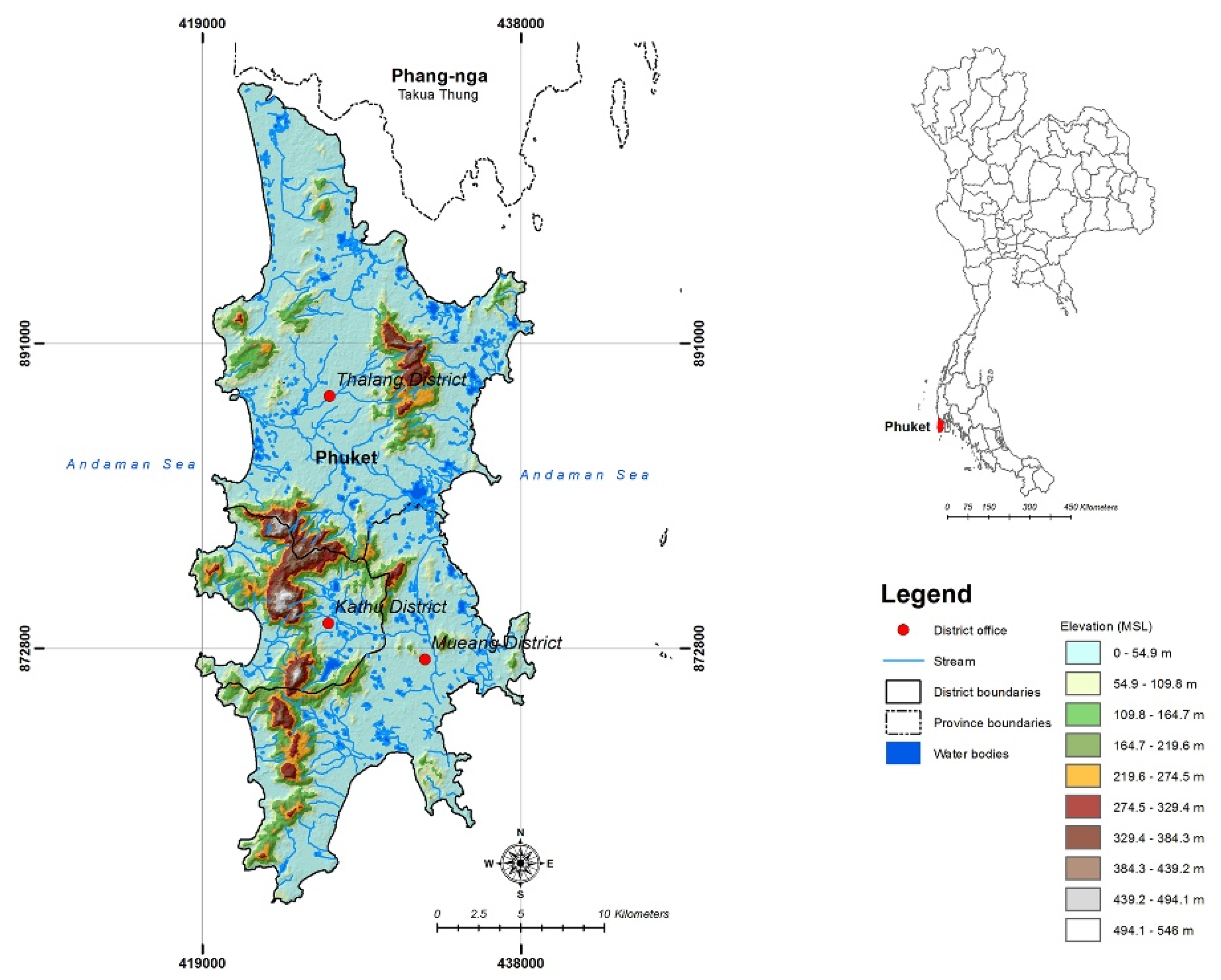
Phuket Island is located in the Andaman Sea of Southern Thailand (Figure 1). With an area of approximately 522 km2, mountains cover about 70% of the island, while the remaining areas of the central and eastern portions of the island are relatively flat. The elevation of the island varies from 0 to 546 m above mean sea level. Phuket Island has a tropical monsoon climate with two distinct seasons; a dry summer season (December–March) and a rainy winter season (April to November) [19]. The average annual rainfall from 2002 to 2011 was 2350 mm [17], while the average annual temperature was 28.1 degrees Celsius [20].
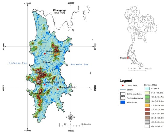
Figure 1.
Elevation and topographic characteristics of the study area.
3. Materials and Methods
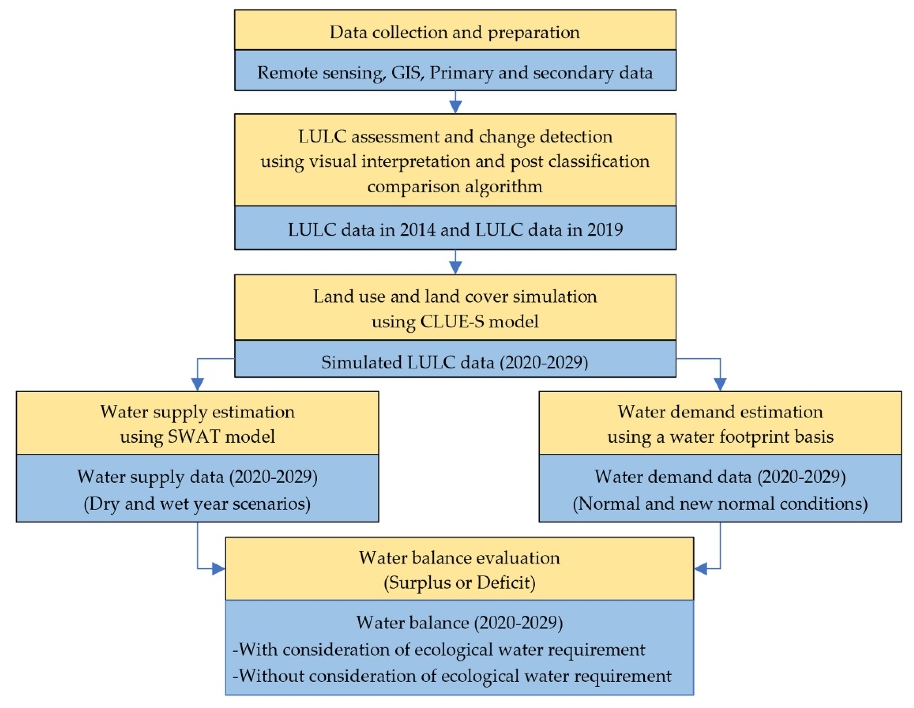
The research methodology workflow was composed of (1) data collection and preparation, (2) LULC assessment and change detection, (3) land use and land cover simulation, (4) water supply estimation, (5) water demand estimation, and (6) water balance evaluation, is displayed in Figure 2. Details of each stage were separately described in the following sections.
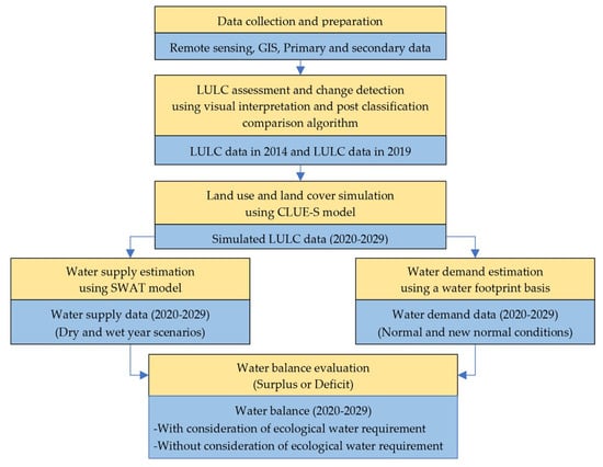
Figure 2.
Workflow of research methodology.
3.1. Data Collection and Preparation
The required remotely sensed data, GIS, and primary and secondary data were collected and prepared for data analysis and modeling, as summarized in Table 1.

Table 1.
Details of data collection and preparation for analysis and modeling in the study.
3.2. Land Use and Land Cover Assessment and Change Detection
The LULC data in 2019 were first visually assessed from Pleiades and SPOT imagery using the element of visual interpretation [22,23]. In this study, the LULC classes were (1) urban and built-up areas, (2) paddy fields, (3) field crops and horticulture, (4) perennial trees and orchards, (5) aquaculture areas, (6) idle land, (7) evergreen forests, (8) mangrove forests, (9) scrub forests, (10) water bodies, and (11) miscellaneous land. Then, the thematic accuracy of the preliminary 2019 LULC map was assessed in a field survey in 2020 using 660 randomly stratified sampling points based on the multinomial distribution theory with a 95% confidence level and 5% precision [24]. Finally, based on the collected and interpreted LULC data, changes were assessed using a post-classification comparison change detection algorithm, which is widely used to extract “from-to” change class information [25,26].
3.3. Land Use and Land Cover Simulation
The CLUE-S (Conversion of Land Use and its Effects at Small regional extent) model was chosen to simulate LULC change between 2020 and 2029. In particular, the Markov Chain model was first used to assess future land demand based on the annual rate of each LULC class from the transition area matrix of LULC change between 2014 and 2019. In general, the Markov chain is a stochastic process model that describes the probability of change from one state to another, i.e., from one land-use type to another, using a transition probability matrix [27]. Then, the selected driving factors of LULC change were applied to identify the LULC type distribution using binomial logistic regression analysis (Equation (1)) for allocating LULC types. In this study, the physical and socio-economic driving factors of LULC change included elevation, slope, distance to water bodies, distance to roads, distance to settlement, soil fertility, population density at the sub-district level, and average income per capita at the sub-district level, which was successfully applied to Phuket Island by Ongsomwang and Boonchoo [28]. Finally, future LULC data were simulated using the CLUE-S model. The conversion matrix, the elasticity of LULC change, and land use demand were simultaneously combined to allocate LULC data according to the driving factors of LULC change for a specific LULC type at a given location. The basic concept and the development of the CLUE-S model were explained in more detail by Verburg et al. [29,30,31].
where Pi is the probability of a grid cell for the considered land-use type in location i, and the Xs are location factors. The coefficients (β) were estimated through logistic regression using the actual land use pattern as the dependent variable.
3.4. Water Supply Estimation
The SWAT model was applied to estimate water supply (water yield) between 2020 and 2029 under dry and wet year scenarios. The SWAT model is a basin-scale, continuous-time model that operates on the basis of daily data and is designed to predict the impact of management on water, sediment, and agricultural chemical yields in ungauged watersheds. The model is physically based, computationally efficient, and capable of continuous simulation over long periods. The major model components include weather, hydrology, soil temperature and properties, plant growth, nutrients, pesticides, bacteria and pathogens, and land management [32,33,34].
3.4.1. Calibration and Validation of SWAT Model
To determine the optimal local model parameters, the Khlong Bang Yai watershed in the study area was chosen as a reference watershed because of the availability of long-term observed hydrologic data. The hydrologic response unit (HRU) was first generated using 20 percent land use, 10 percent soil, and 20 percent slope thresholds, which are suitable for most applications [35,36]. Weather data (precipitation, temperature, solar radiation, wind speed, and humidity) collected by six meteorological stations of the Thai Meteorological Department and Royal Irrigation Department between 1996 and 2019 were prepared and input into the model. Then, a sensitivity analysis was conducted to determine the influence of parameters on estimating total flow to identify the most sensitive parameters in the study area. Seven critical parameters—curve number at moisture condition II, available soil water capacity, soil evaporation compensation factor, surface runoff lag coefficient, baseflow alpha factor, groundwater “revap” coefficient, and groundwater delay, which affect surface runoff and baseflow as suggested by many researchers [6,37,38,39,40,41,42,43]—were analyzed using t-statistics in the SWAT-CUP software, with p-values considered significant at the 5% significance level.
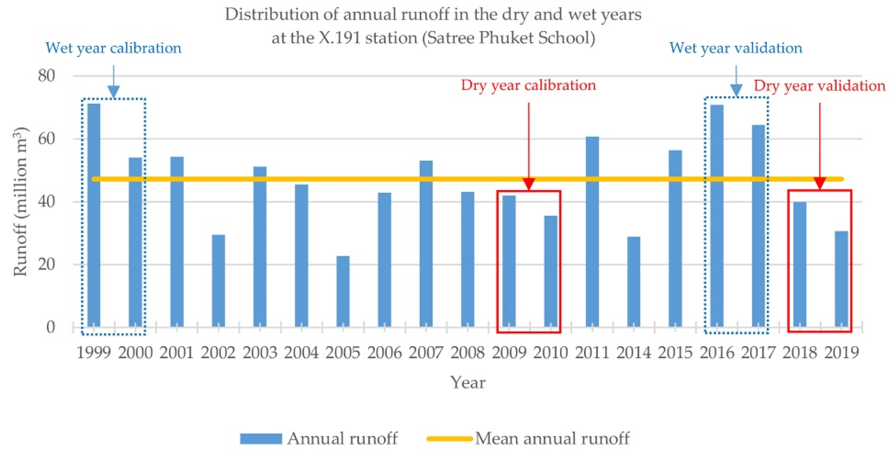
After that, these parameters were systematically calibrated to identify the optimal local model parameters for water yield estimation according to annual runoff data at the X.191 station of the Khlong Bang Yai watershed under dry and wet year conditions. Dry and wet year conditions were defined based on the long-term mean annual runoff between 1999 and 2019 at the X.191 station (Figure 3). Any year in which annual runoff was higher than the mean annual runoff was identified as a wet year. Conversely, any year in which the annual runoff was less than the mean annual runoff was identified as a dry year. Then, the local model parameters identified in the calibration phase were further applied to validate the model. Table 2 summarizes the essential data required for the model calibration and validation periods under dry and wet year conditions.
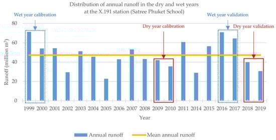
Figure 3.
Distribution of annual runoff in the dry and wet year conditions at the X.191 station.
Table 2.
Essential data required for model calibration and validation under dry and wet year conditions.
Furthermore, the RMSE-observations standard deviation ratio (RSR) [44], Nash–Sutcliffe efficiency (NSE) [45], and percent bias (PBIAS) [46], as shown in Equations (2)–(4), were determined to evaluate the performance of the model, where good performance is defined by expected threshold values of ≤0.60, ≥0.65, and ≤±15% in the model calibration and validation phases (Table 3).
where Ei is the estimated value, and Oi is the observed value at time i. is the mean of the individual observations of Oi, and n is the number of observations.
Table 3.
Model performance scale.
3.4.2. Water Yield Estimation Using SWAT Model
The optimal local parameters of dry and wet year conditions from the model calibration phase were applied to estimate the time-series water yield between 2020 and 2029 for Phuket Island with representative rainfall data under dry and wet year scenarios.
To identify rainfall data for dry and wet year scenarios, long-term historical rainfall data were obtained from the Thai Meteorological Department for Phuket and Phuket Airport stations from 1999 to 2019. According to the data, 2004 or 2005 can be used as representative dry years. However, rainfall data at Krabi and Takua Pa stations were unavailable for these years, so the lowest rainfall data in 2019 were chosen to represent the dry year scenario. The highest rainfall value was found in 2016, which was used to represent the wet year scenario (Figure 4). Thus, the time-series water yield between 2020 and 2029 under the dry and wet year scenarios in this study was estimated based on weather data in 2019 and 2016, respectively.
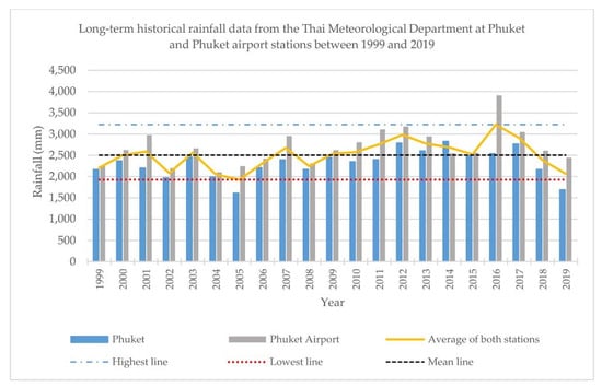
Figure 4.
Long-term historical rainfall data at Phuket and Phuket Airport stations between 1999 and 2019.
3.5. Water Demand Estimation
Phuket Island’s water demand between 2020 and 2029 was estimated under normal and new normal (COVID-19 pandemic) conditions for three primary consumption activities: residential, tourist, and agriculture and forest use.
3.5.1. Residential Water Demand
Under normal and new normal conditions, the number of people (registered and non-registered populations) was estimated based on historical data using linear regression analysis. The registered population was estimated based on historical data between 2012 and 2019 from the DOPA database, Ministry of Interior. To extract the non-registered population, census data were estimated based on historical data between 1980 and 2010 from NSO. Finally, residential water demand was estimated in different community types using the water consumption rate from the Royal Irrigation Department [48], as summarized in Table 4.
Table 4.
Water consumption rates in different community types.
3.5.2. Tourist Water Demand
The number of tourists under the normal condition was estimated using linear regression analysis based on historical data between 2010 and 2019. In contrast, future tourist projections by the Economics Tourism and Sports Division, Ministry of Tourism and Sports, were adopted for tourist numbers under the new normal conditions (COVID-19 pandemic) [4]. In this condition, three future tourist scenarios were estimated for 2021, 2022, and 2023 assuming 45%, 65%, and 85% of the tourists in 2019, respectively. The number of tourists between 2024 and 2029 was based on the same data as the normal condition. Finally, tourist water demand between 2020 and 2029 under normal and new normal conditions was estimated according to the tourist type (tourists and excursionists) based on the modified water consumption rate of Pansawad (1997) and the Department of Public Works and Town and Country Planning (1993), as cited by Royal Irrigation Department [48] and Srichai et al. [49], with an average length of stay of four days [3] (Table 5).
Table 5.
The water consumption rates of tourists and excursionists.
3.5.3. Water Demand for Agriculture and Forest Uses
Under normal and new normal conditions, the water demand for agriculture and forest uses was estimated based on the evapotranspiration coefficient and reference evapotranspiration [50], as shown in the following equation.
where ETc is the water requirement (mm/day), Kc is the evapotranspiration coefficient, and ETo is reference evapotranspiration (mm/day).
In particular, the water demand for agriculture and forest use was calculated based on the area of each agriculture and forest type, the evapotranspiration coefficient (Kc) (see Appendix A Table A1), and reference evapotranspiration using the Penman–Monteith method (see Appendix A Table A2).
In this analysis, the water balance between 2020 and 2029 was evaluated with and without the consideration of ecological water requirements based on the estimated water supply and demand under two different scenarios (dry year and wet year) and two different conditions (normal and new normal).
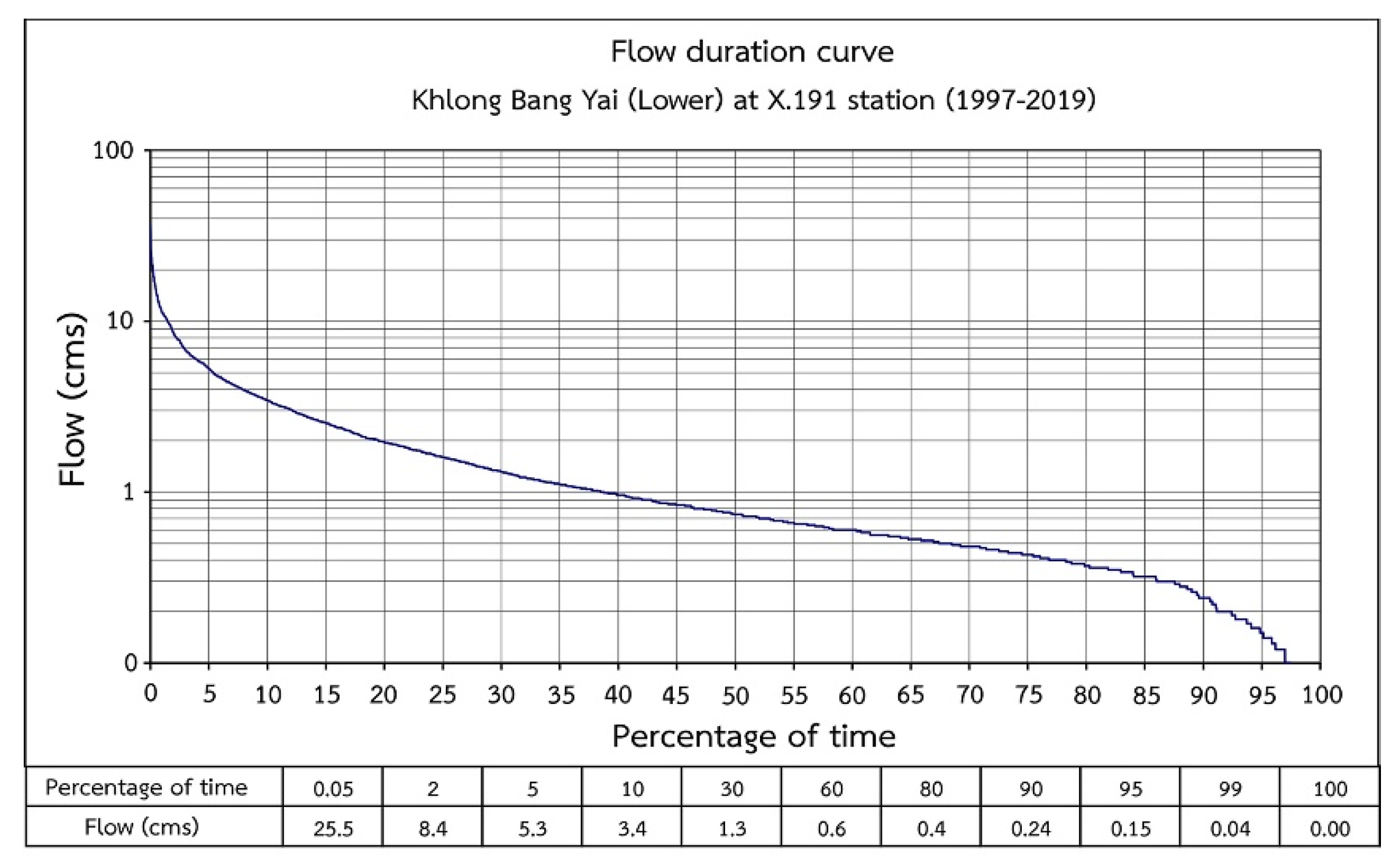
In particular, the annual and monthly water balance without the consideration of ecological water requirements was evaluated based on the annual and average monthly water supply derived from the SWAT model. Additionally, the annual and monthly water balance with the consideration of ecological water requirements was evaluated based on water supply, which was derived from the SWAT model for 70% of the time and 0.5 m3 per second of flow (standard criteria) under the criteria of minimum water from the flow duration curve at the outlet at X.191 station of Khlong Bang Yai watershed, as suggested by Southern Region Irrigation Hydrology Center, Royal Irrigation Department [51] (see Figure 5 and Table 6). On this basis, Phuket Island’s annual ecological water requirement was 147.64 million m3 per year, while the monthly ecological water requirement was 12.30 million m3 per month.
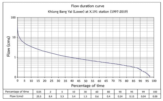
Figure 5.
The flow duration curve of X.191 station (Satree Phuket School). Source: Southern Region Irrigation Hydrology Center, Royal Irrigation Department [51].
Table 6.
The criteria of minimum water from the flow duration curve.
4. Results and Discussion
4.1. Land Use and Land Cover Assessment and Change Detection
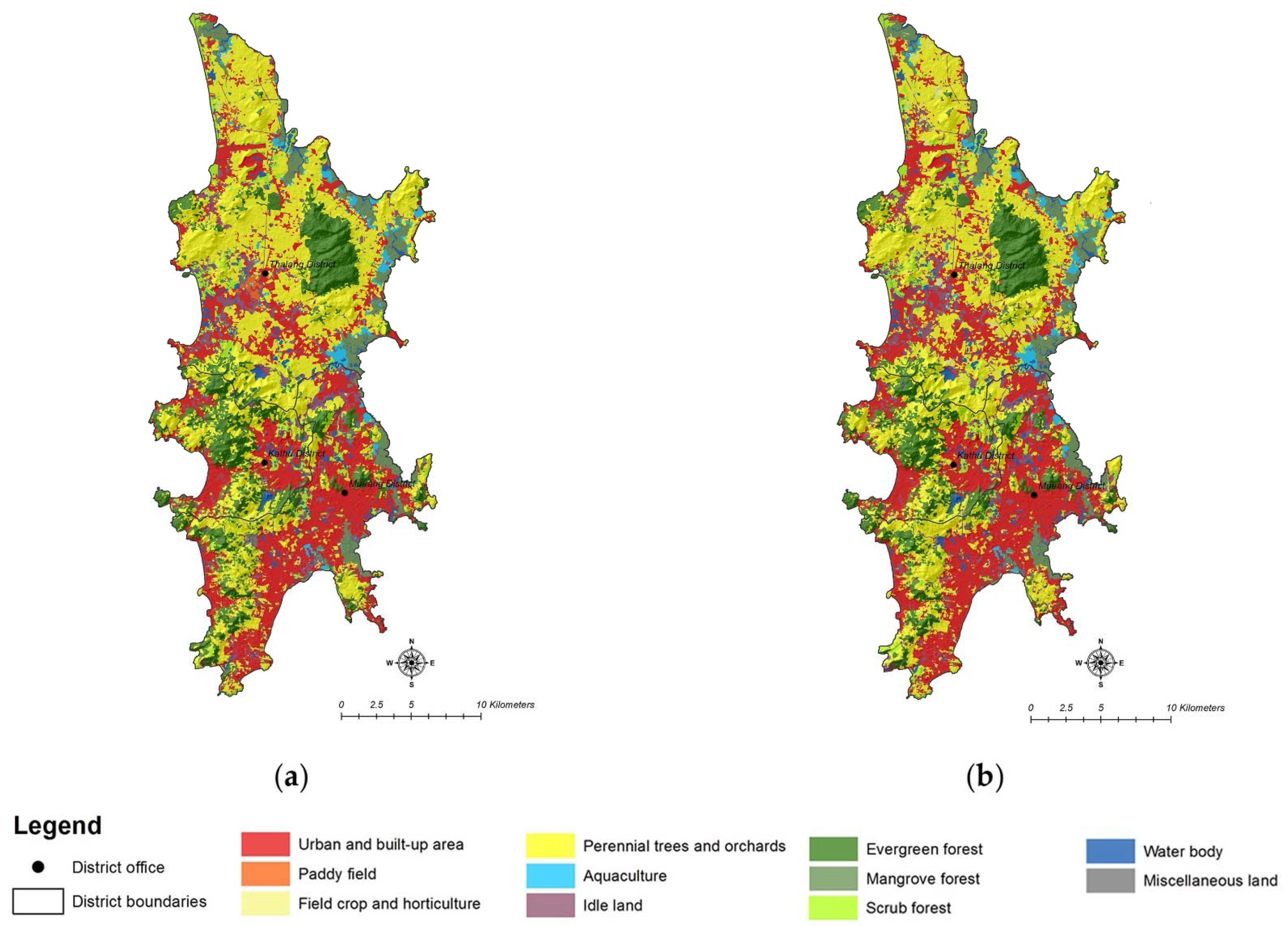
The area and percentage of the LULC data in 2014 and 2019 are summarized in Table 7, and the spatial distribution of LULC is mapped in Figure 6. Results indicate that three LULC types are dominant on the Island. These include perennial trees and orchards, urban and built-up areas, and evergreen forest, which covered 37.7%, 24.0%, and 15.5%, respectively, in 2014 and 35.3%, 27.1%, and 14.2%, respectively, in 2019.
Table 7.
Area and percentage of LULC data in 2014 and 2019.

Figure 6.
Spatial distribution of LULC classification: (a) LULC in 2014; (b) LULC in 2019.
The results of the accuracy assessment of the LULC map in 2019 are reported in Table 8. The overall accuracy and the Kappa hat coefficient of the LULC map in 2019 are 96.06% and 95.15%, respectively. The producer’s accuracy (PA), which represents omission error, varies from 87.50% to 100%, and the significant omission error occurs in idle land, with a value of 12.5%. At the same time, the user’s accuracy (UA), which represents commission error, varies from 87.50% to 100%, and the significant commission error occurs in the paddy field with a value of 12.5%. According to Fitzpatrick-Lins, a Kappa hat coefficient of more than 80% represents a strong agreement (high accuracy) between the classified and reference maps [52]. Additionally, an overall accuracy of more than 85% for the LULC map in 2019 is regarded as an acceptable result [53].
Table 8.
Error matrix and accuracy assessment of the LULC map in 2019.
Moreover, the transition area matrix of LULC change between 2014 and 2019 is presented in Table 9. These results indicate that the increase in urban and built-up areas in 2019 was due to the conversion of perennial trees and orchards and idle land in 2014. In addition, the increase in perennial tree and orchard areas in 2019 was due to the conversion of evergreen and scrub forests in 2014. Similarly, the increase in idle land area in 2019 was due to the conversion of perennial trees and orchards in 2014.
Table 9.
LULC change between 2014 and 2019 as a transition area matrix.
In contrast, perennial trees and orchards in 2014 were converted into idle land, field crops and horticulture, scrub forest, evergreen forest, miscellaneous land, and water bodies in 2019. Additionally, idle land in 2014 was converted into urban and built-up areas, perennial trees and orchards, and scrub forest in 2019. Similarly, areas of evergreen forest in 2014 were converted into perennial trees and orchards and scrub forests in 2019.
Furthermore, according to the pattern of LULC change identified in a previous study by Boonchoo [21] and the current study, the urban and built-up areas will continuously increase in the near future. Several potential causes of the transformation of the land use pattern in Phuket Island have been identified, such as rapid economic development, registered and non-registered population growth, and tourist growth. As a result, hotels and recreational and commercial areas have been constructed to support tourism. Phuket Island’s urban and built-up areas have been primarily expanded by converting perennial trees and orchards and idle land. This finding is consistent with previous studies [54,55], which stated that most agricultural land and vegetation areas were transformed into urban and built-up areas to meet people’s demands, leading to the LULC change.
4.2. Land Use and Land Cover Simulation
Table 10 reports the results of binary logistic regression analysis, which was carried out to identify the LULC type distribution according to the driving factors of LULC change after the multicollinearity test. The top three significant driving factors for the allocation of specific LULC types in the study area are the distance to water bodies, elevation, and distance to roads. The significant driving factors identified for each LULC type for LULC allocation were further used in the CLUE-S model during the simulation process.
Table 10.
Multiple linear regression equation of each LULC type and area under the curve value from logistic regression analysis.
In addition, the area under the curve (AUC) values derived for allocating each LULC type using binary logistic regression analysis are between 0.65 and 0.94, which means that the difference between simulated and actual LULC is acceptable, and the model has fair to outstanding discrimination ability [56]. The simulated LULC data between 2020 and 2029 and their distribution are summarized and presented in Table 11 and Figure 7.
Table 11.
Area of simulated LULC data between 2020 and 2029.
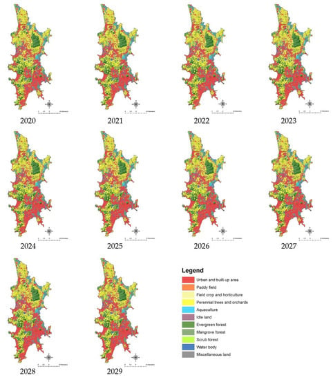
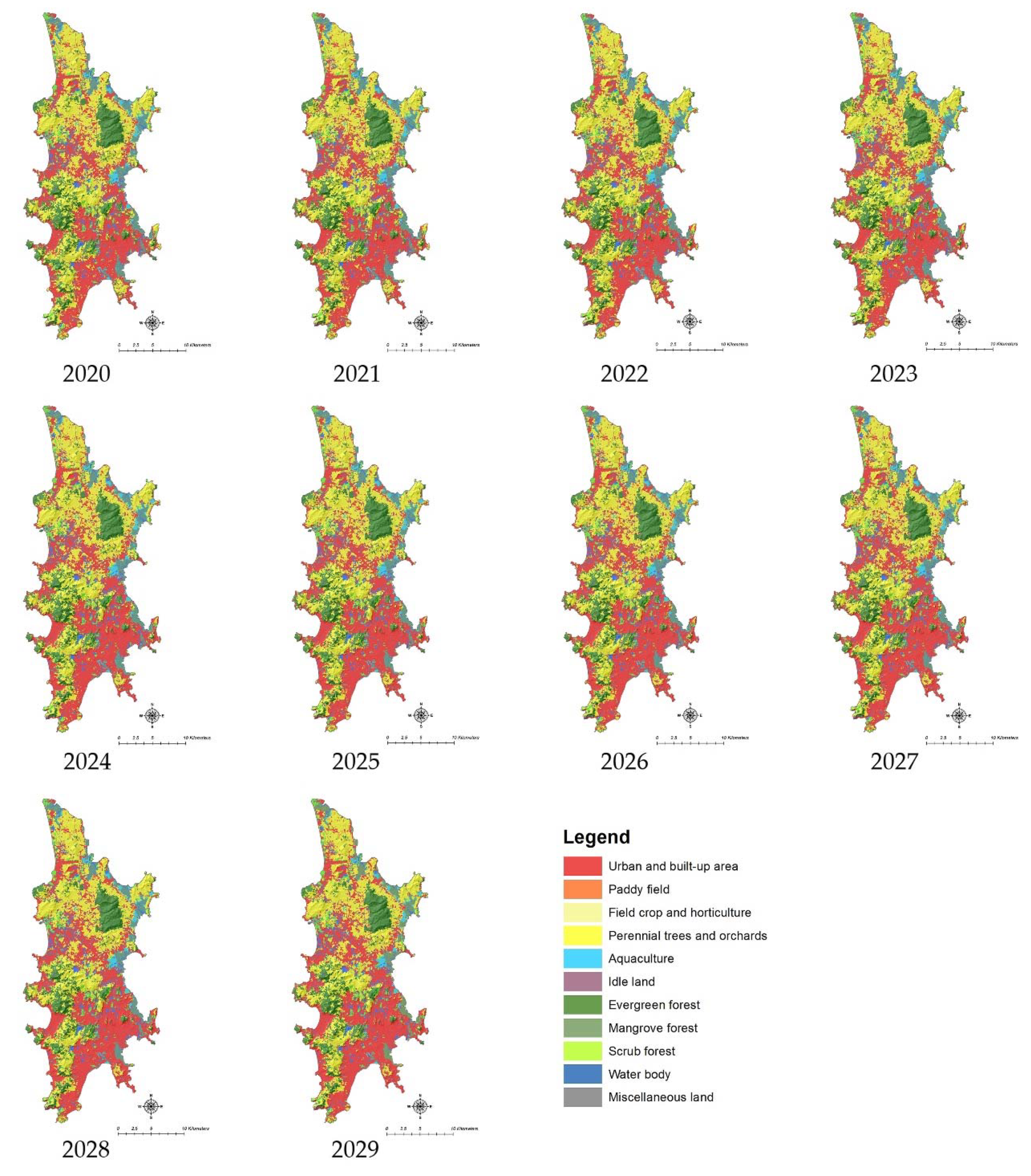
Figure 7.
Spatial distribution of the simulated LULC scenario between 2020 and 2029.
According to the results, the LULC types that will increase in 2029 are urban and built-up areas, field crops and horticulture, idle land, scrub forest, and water bodies. On the contrary, the LULC types that will decrease in 2029 are paddy fields, perennial trees and orchards, aquaculture, evergreen forest, mangrove forest, and miscellaneous land. These findings are based on the driving factors of LULC change, conversion matrix, and elasticity of LULC change and their land requirements, which were applied to the CLUE-S model for LULC simulation between 2020 and 2029.
In this study, a slight difference was found between the land demand (required land area) and the simulated area of each LULC type in 2029. The deviation between the land demand and the simulated area in 2029 is −0.01 km2 because the deviation value depends on the iteration driving factors of each LULC type, which indicates the different maximum allowances between the required and allocated areas of LULC types under the CLUE-S model [57,58,59].
4.3. Sensitivity Analysis and Model Calibration and Validation
The results of the sensitivity analysis are reported in Table 12. According to the results, available soil water capacity (SOL_AWC) is the most sensitive parameter in the Khlong Bang Yai watershed. Thus, the available soil water capacity, which is the soil’s capacity to hold water available for plant use and reflects the soil’s capacity for water storage [60,61], was the main value adjusted in the model calibration stage. In addition, the curve number at moisture condition II (CN2), soil evaporation compensation factor (ESCO), and groundwater “revap” coefficient (GW_REVAP), which relate to surface runoff and baseflow, were slightly modified in this study.
Table 12.
SWAT parameter sensitivity to monthly streamflow at the X.191 station.
The optimal model parameters in the calibration period under dry and wet year conditions are reported in Table 13. The results indicate that the optimal value of available soil water capacity (SOL_AWC) varies according to soil type. Likewise, the curve number at moisture condition II (CN2) depends on land use, soil, and slope.
Table 13.
Optimal parameter values of SWAT model for hydrologic component estimation under dry and wet year conditions.
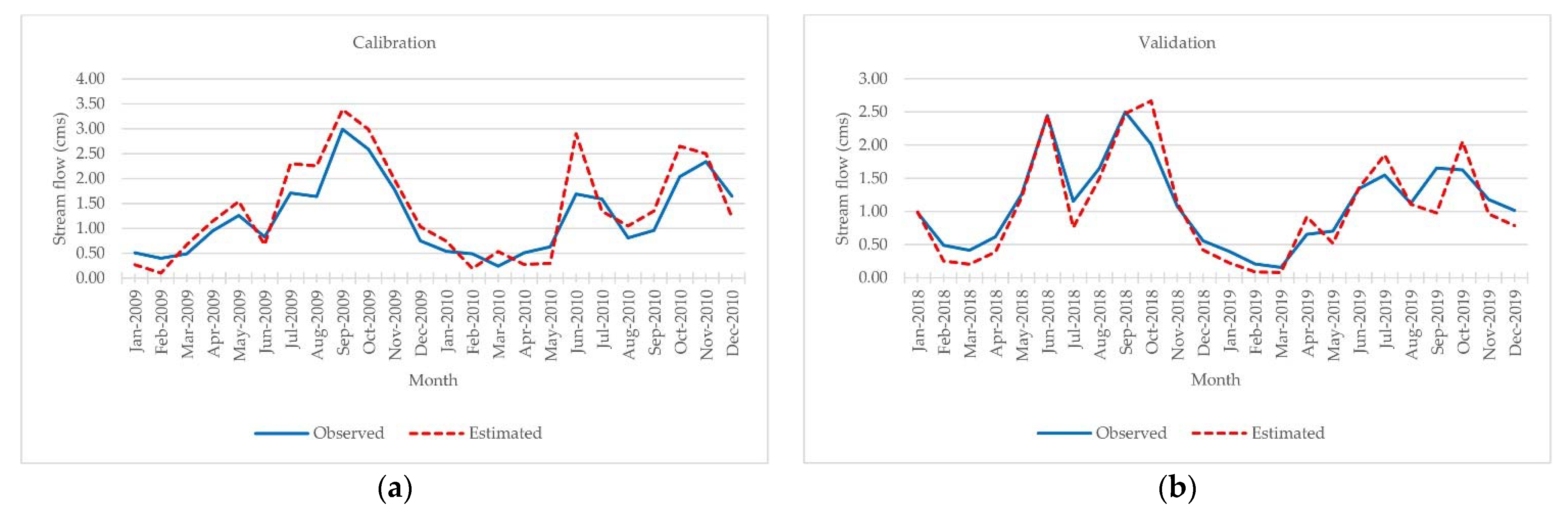
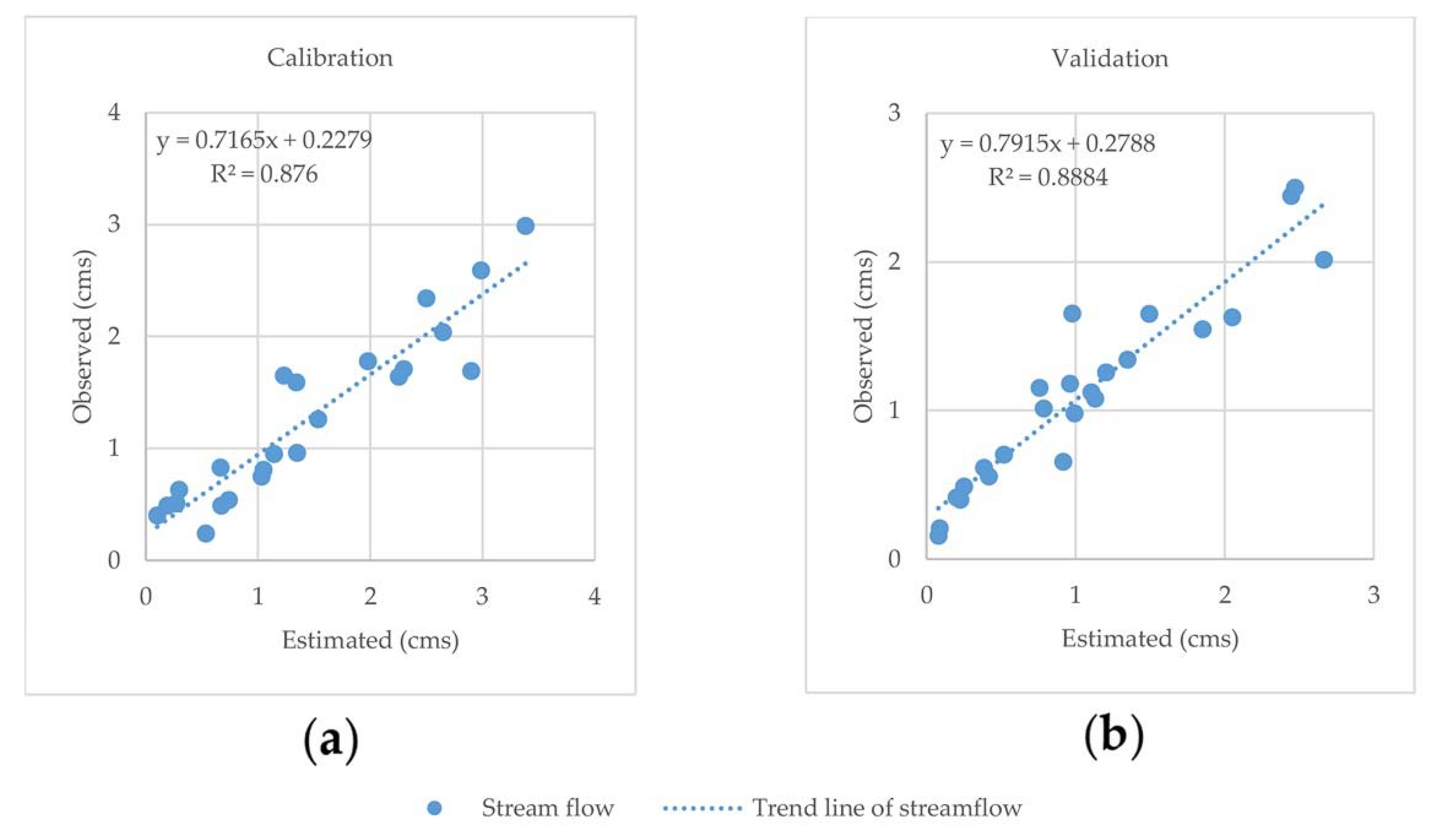
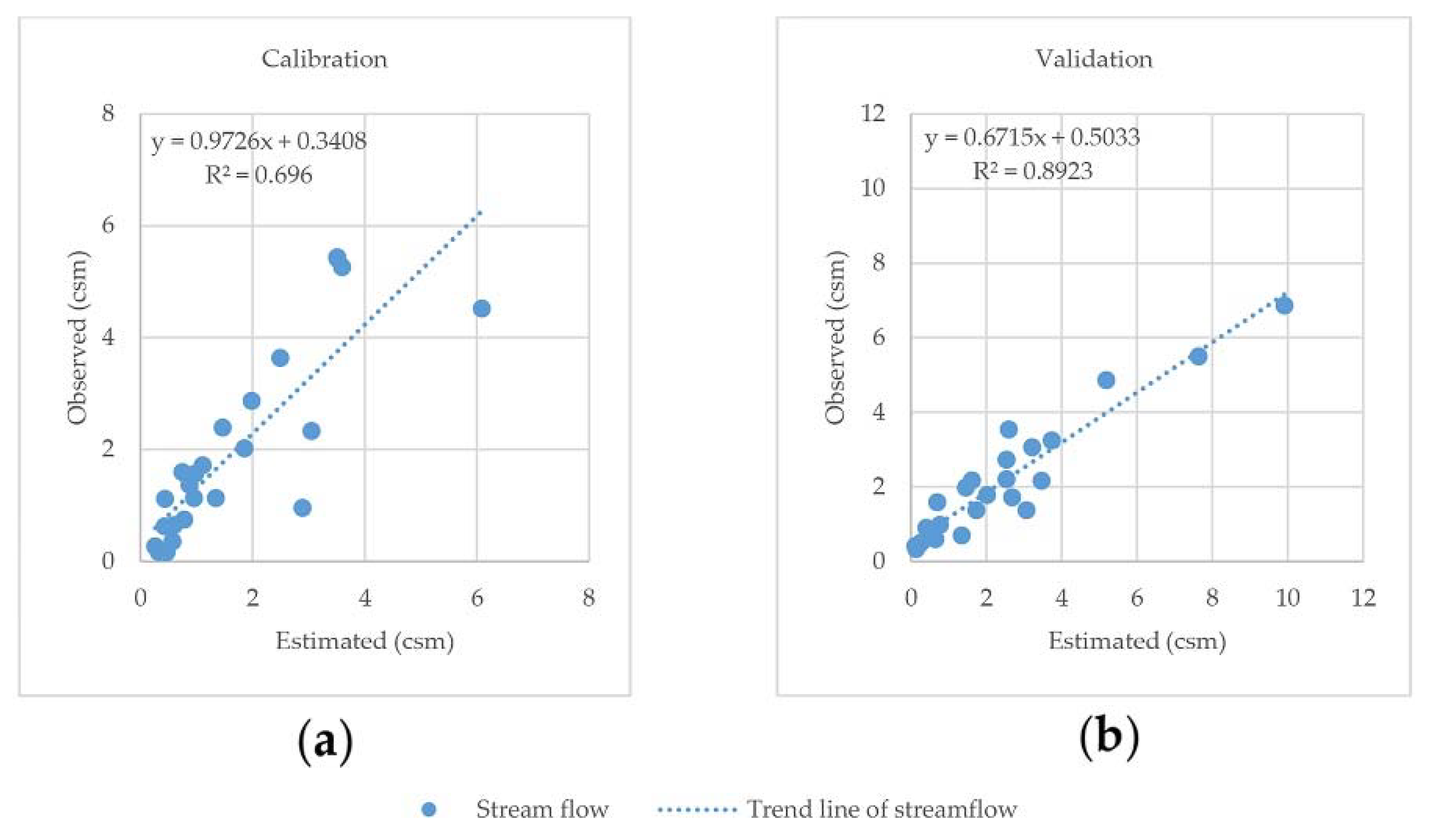
Furthermore, Table 14 and Figure 8 summarize the SWAT model’s performance for the dry year condition in the calibration and validation periods based on the observed and estimated hydrologic data at the X.191 station. According to the three statistical values, the model shows good performance in the calibration period and very good performance in the validation period, according to the model performance scale of Moriasi et al. [47]. The R2 values in the calibration and validation periods are 0.88 and 0.89, as shown in Figure 9.
Table 14.
Performance of the SWAT model for water yield estimation in calibration and validation periods under the dry year condition.
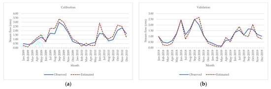
Figure 8.
Monthly observed and estimated streamflow at Khlong Bang Yai watershed under the dry year condition: (a) calibration period; (b) validation period.
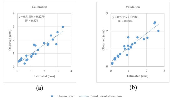
Figure 9.
Scatter plot between observed and estimated streamflow at Khlong Bang Yai watershed under the dry year condition: (a) calibration period; (b) validation period.
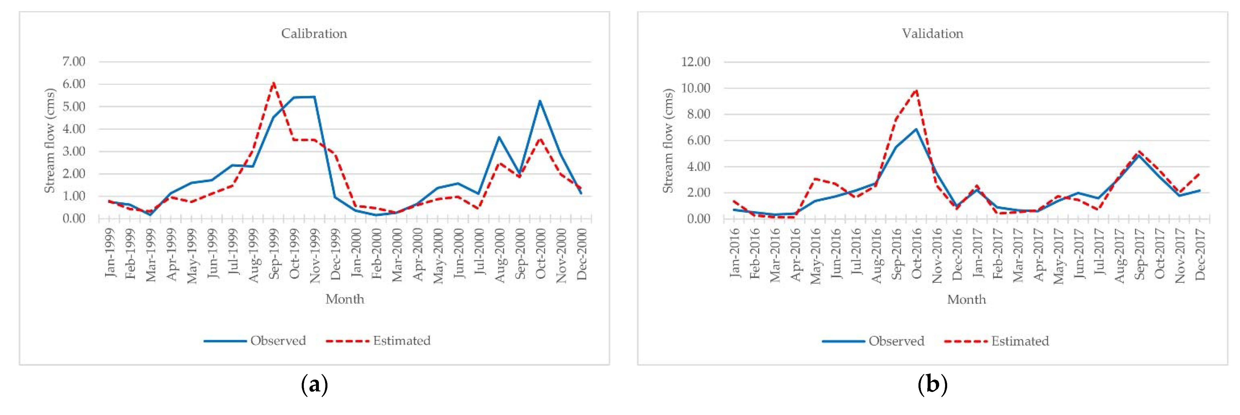
The SWAT model’s performance for the wet year condition in the calibration and validation periods based on the estimated and observed hydrologic data at the X.191 station is summarized in Table 15 and Figure 10. According to the three statistical values, the model shows good performance in the calibration and validation periods, as suggested by Moriasi et al. [47]. Additionally, the R2 values in the calibration and validation periods are 0.70 and 0.89, as shown in Figure 11.
Table 15.
Performance of the SWAT model for water yield estimation in calibration and validation periods under the wet year condition.
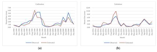
Figure 10.
Monthly observed and estimated streamflow at Khlong Bang Yai watershed under the wet year condition: (a) calibration period; (b) validation period.
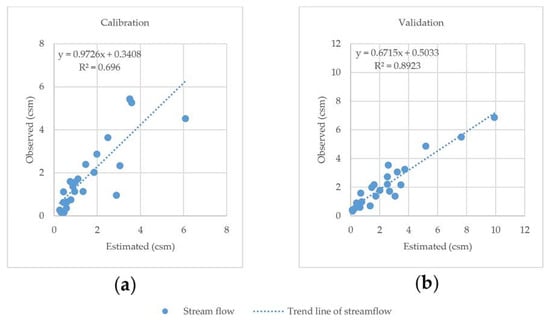
Figure 11.
Scatter plot between observed and estimated streamflow at Khlong Bang Yai watershed under the wet year condition: (a) calibration period; (b) validation period.
4.4. Estimation of Water Yield between 2020 and 2029
The optimal local parameters from the dry year condition were further applied to estimate the water yield between 2020 and 2029 under the dry year scenario. The optimal local parameters from the wet year condition were also applied to estimate the water yield in the same period under the wet year scenario.
4.4.1. Water Yield Estimation under Dry Year Scenario
Table 16 displays the annual water yield of simulated LULC between 2020 and 2029 under the dry year scenario with 2376.50 mm rainfall. According to the results, the estimated annual water yield varies from 967.36 mm (505.01 million m3) to 999.49 mm (521.79 million m3), with an average annual water yield of 981.17 mm (512.22 million m3). In addition, the estimated annual evapotranspiration varies from 1281.50 mm to 1298.60 mm, with an average annual evapotranspiration value of 1291.67 mm. These findings indicate that LULC change affects water yield through its hydrologic component and evapotranspiration because, as significant input data for water yield estimation, rainfall data are fixed, while LULC data are dynamic.
Table 16.
Annual water yield of Phuket Island between 2020 and 2029 under dry year scenario.
In addition, Table 17 presents the estimated monthly water yield between 2020 and 2029 under the dry year scenario. According to these results, the average monthly water yield in the summer season (December–March) varies from a minimum of 1.84 million m3 in March to a maximum of 31.86 million m3 in December. The average monthly water yield in the rainy season (April–November) varies from a minimum of 16.10 million m3 in May to a maximum of 102.26 million m3 in October.
Table 17.
Monthly water yield of Phuket Island between 2020 and 2029 under dry year scenario.
4.4.2. Water Yield Estimation under Wet Year Scenario
Table 18 displays the annual water yield of simulated LULC between 2020 and 2029 under the wet year scenario with 3686.00 mm rainfall. According to the results, the estimated annual water yield varies from 2347.42 mm (1225.48 million m3) to 2379.23 mm (1242.08 million m3), with an average annual water yield of 2361.84 mm (1233.00 million m3). In addition, the estimated annual evapotranspiration varies from 934.30 mm to 936.10 mm, with an average annual evapotranspiration value of 935.27 mm. The annual evapotranspiration of Phuket Island under this scenario is relatively stable. Additionally, as with the dry year scenario, these findings indicate that LULC change affects water yield through its hydrologic component and evapotranspiration because, as significant input data for water yield estimation, rainfall data are fixed.
Table 18.
Annual water yield of Phuket Island between 2020 and 2029 under the wet year scenario.
Furthermore, the monthly water yield estimation under the wet year scenario is reported in Table 19. The results show that the average monthly water yield in the summer season (December–March) varies from a minimum of 4.95 million m3 in March to a maximum of 58.92 million m3 in December. The average monthly water yield in the rainy season (April–November) varies from a minimum of 2.80 million m3 in April to a maximum of 286.47 million m3 in October.
Table 19.
Monthly water yield of Phuket Island between 2020 and 2029 under wet year scenario.
4.5. Effect of LULC Change on Water Yield
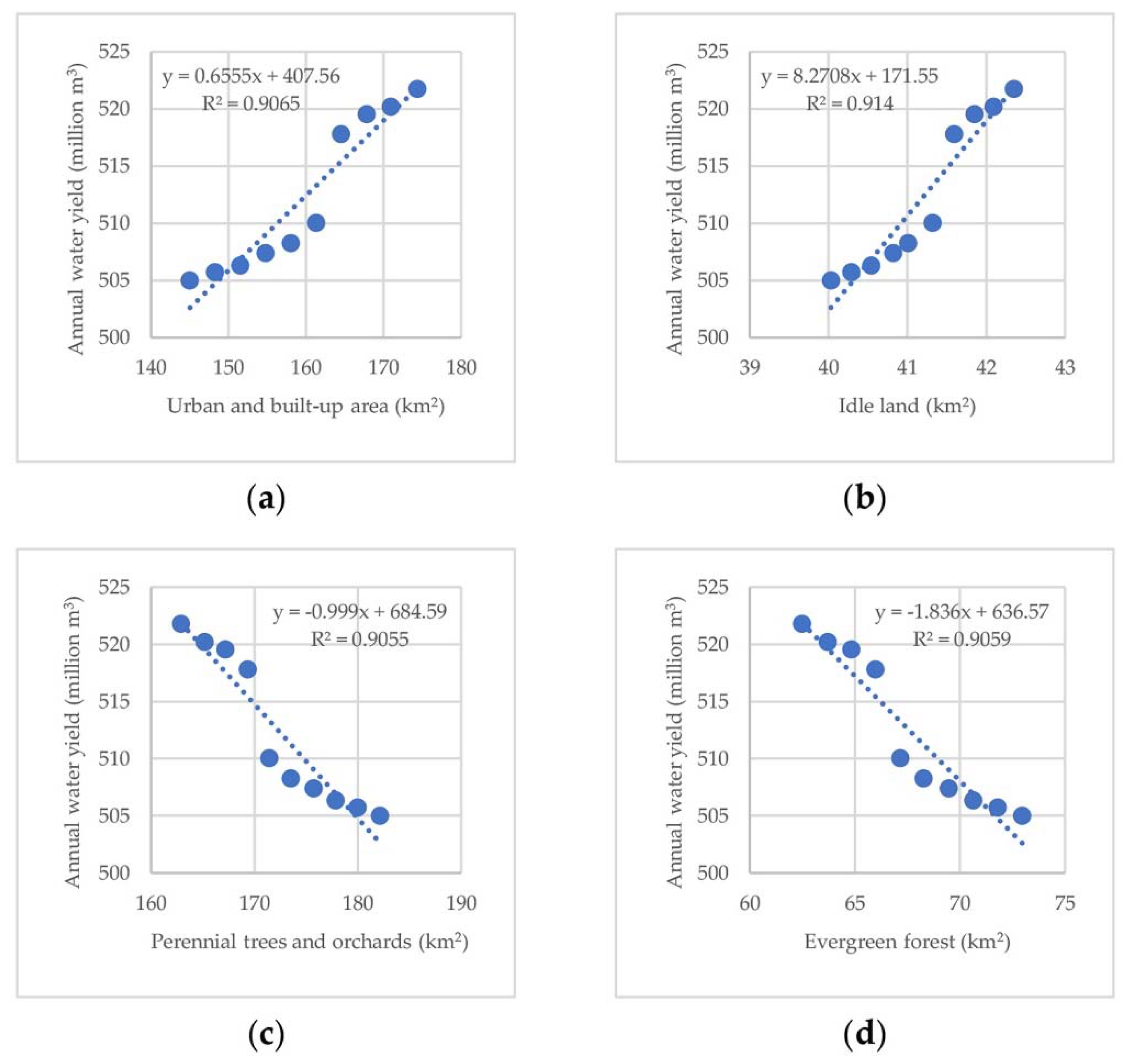
Simple linear regression analysis was applied to identify the effect of LULC change on water yield (see Appendix A for input data in Table A3). The simple linear equations between water yield and specific dominant LULC types under dry and wet scenarios are displayed in Figure 12 and Figure 13.
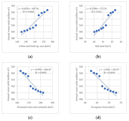
Figure 12.
Simple linear regression analysis between LULC type and water yield under dry year scenario.
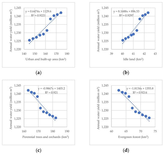
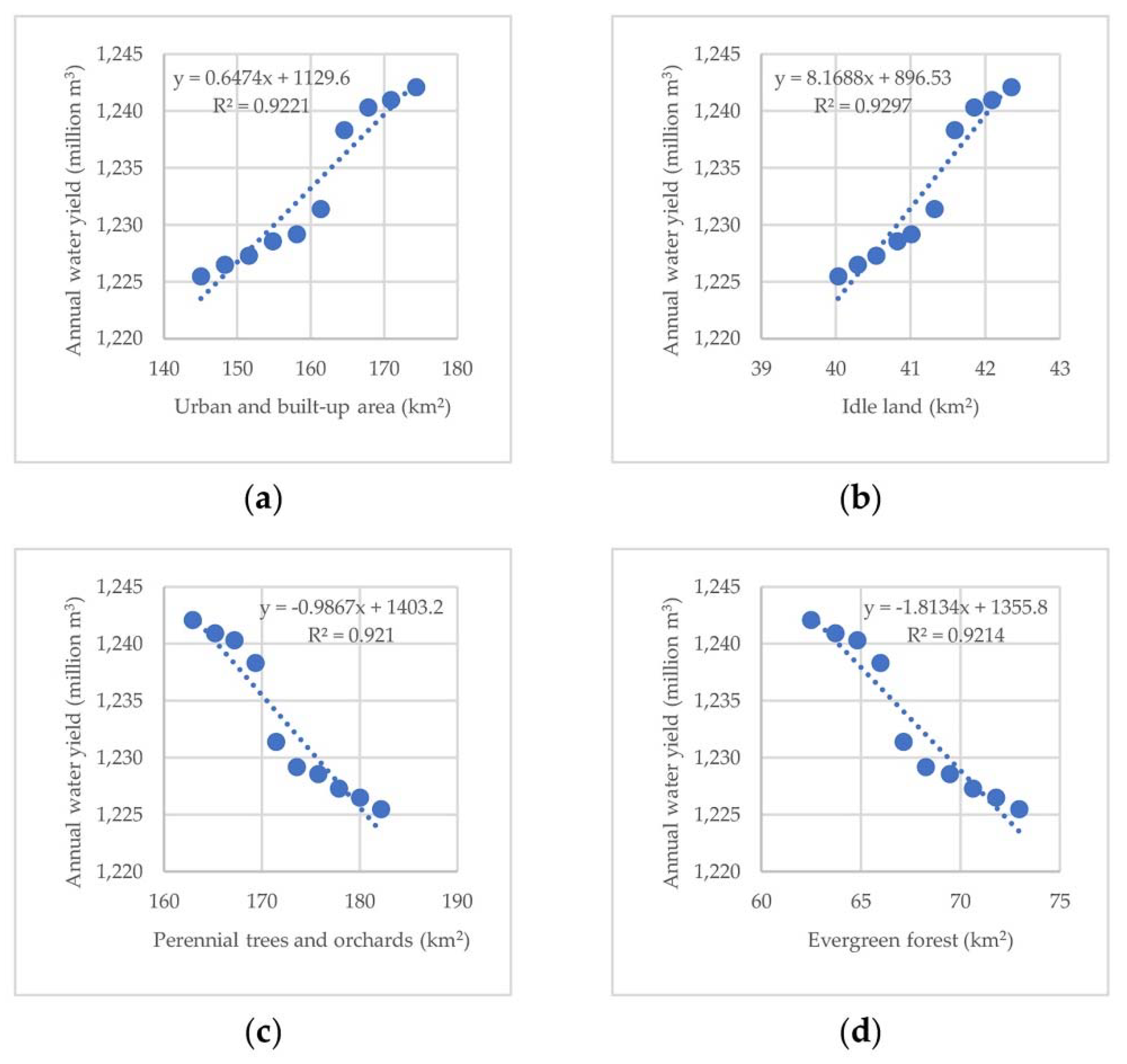
Figure 13.
Simple linear regression analysis between LULC type and water yield under wet year scenario.
The results show that annual water yield in the dry and wet year scenarios is positively correlated with urban and built-up areas, with R2 values of 0.91 and 0.92, respectively (Figure 12a and Figure 13a). This finding indicates that when urban and built-up areas increase, water yield increases. This phenomenon is expected because surface runoff, as a significant hydrologic component of water yield, will increase when urban and built-up areas with impervious surfaces increase. Likewise, annual water yield in both scenarios is positively correlated with idle land (abandoned and fallowed fields), with R2 values of 0.91 and 0.93, respectively (Figure 12b and Figure 13b). This finding shows that when idle land increases, water yield increases.
On the contrary, annual water yield in the dry and wet year scenarios has a high negative correlation with perennial trees and orchards, with R2 values of 0.91 and 0.92, respectively (Figure 12c and Figure 13c). This finding indicates that when perennial trees and orchards increase, water yield decreases. This phenomenon is expected because surface runoff will decrease when areas are covered by vegetation. Likewise, annual water yield in both scenarios shows a high negative correlation with evergreen forest, with R2 values of 0.91 and 0.92, respectively (Figure 12d and Figure 13d). This finding confirms the influence of LULC change on the surface runoff in the watershed.
These findings are comparable to those of other studies. To determine the impact of land-use change on surface runoff in Huay Tung Lung Watershed of Mun Basin, Ongsomwang and Kunto applied the SWAT model to estimate surface runoff and the CA Markov model to predict land-use changes. They found that land-use changes in the watershed area directly affected surface runoff [62]. Ayivi and Jha applied the SWAT model to estimate water balance and water yield in the Reedy Fork-Buffalo Creek Watershed in North Carolina, USA. They found that the surface runoff and water yield at the watershed outlet were significantly increased due to the conversion of forest and grassland to impervious surfaces [41]. Likewise, Hu et al. integrated GIS and remote sensing methods with the SCS-CN model to assess the impact of land-use change on surface runoff in Beijing, China. They found that changes in surface runoff were positively correlated with impervious land changes but negatively correlated with woodland, grassland, farmland, and water changes [63].
Similarly, Puno et al. applied the SWAT model to determine the hydrologic responses to land cover and climate change in the Muleta watershed, Bukidnon, Philippines. Their results showed that urbanization influenced the increase in surface runoff, evapotranspiration, and baseflow. An increase in forest vegetation resulted in a minimal decrease in baseflow and surface runoff [64].
4.6. Estimation of Water Demand between 2020 and 2029
The main results of water demand estimation between 2020 and 2029 under normal and new normal (COVID-19 pandemic) conditions are separately described below for three primary consumption activities: residential, tourist, and agriculture and forest uses.
4.6.1. Residential Water Demand
Table 20 reports the annual residential water demand in different community types between 2020 and 2029 under normal and new normal conditions.
Table 20.
Annual residential water demand in different community types between 2020 and 2029.
The top three areas with the highest average total residential water demand are Phuket City Municipality (10.90 million m3), Kathu Town Municipality (3.79 million m3), and Vichit Sub-district Municipality (3.77 million m3). The top three areas with the lowest average total residential water demand are Kamala Sub-district (0.20 million m3), Sakhu Sub-district (0.21 million m3), and Cherngtalay Sub-district (0.33 million m3).
According to the results, Phuket Island’s average annual residential water demand will continuously increase between 2020 and 2029. Notably, residential water demand in urban areas is higher than in rural areas of Phuket Island. This finding indicates that growth rates of the population and consumption patterns differ between urban and rural areas of Phuket Island, as suggested by Boretti and Rosa [65]. They found that increasing water demand follows population growth, economic development, and changing consumption patterns.
Furthermore, these findings are comparable to those of other studies. For instance, Wijitkosum and Sriburi studied the effect of urban expansion of Nakhon Ratchasima City, the regional center of Northeastern Thailand, on water demand and water usage in the Lam Ta Kong Watershed. The results showed that urbanization affected the water usage pattern, and people’s high living standards continuously increased the water consumption rate [66]. Similarly, Liu et al. integrated weighting methods to evaluate urban and rural water poverty in Northwest China. The results showed that urban areas characterized by rapid economic growth displayed accelerated improvement in water poverty [67].
4.6.2. Tourist Water Demand
Tourist water demand between 2020 and 2029 was estimated using the water consumption rate for a four-day stay and the number of tourists under normal and new normal conditions. Under normal conditions, the number of tourists varies from 16,534,377 people to 21,671,107 people, with an average of 18,828,364 tourists per year. Tourist water demand will increase from 18,861,284 m3 in 2020 to 24,757,427 m3 in 2029, with an average tourist water demand of 21,493,892 m3 (Table 21).
Table 21.
The number of tourists and water demand between 2020 and 2029 under normal conditions.
Conversely, the number of tourists under new normal conditions varies from 4,003,290 people to 21,671,107 people, with an average of 15,263,706 tourists per year. In addition, tourist water demand varies from 4,524,179 m3 to 24,757,427 m3, with an average tourist water demand of 17,417,294 m3 (Table 22). Under new normal conditions, the tourist water demand will drop between 2020 and 2023 due to the COVID-19 pandemic, but it will increase from 2024 to 2029 when the COVID-19 pandemic is under control and normal conditions are re-established.
Table 22.
The number of tourists and water demand between 2020 and 2029 under new normal conditions.
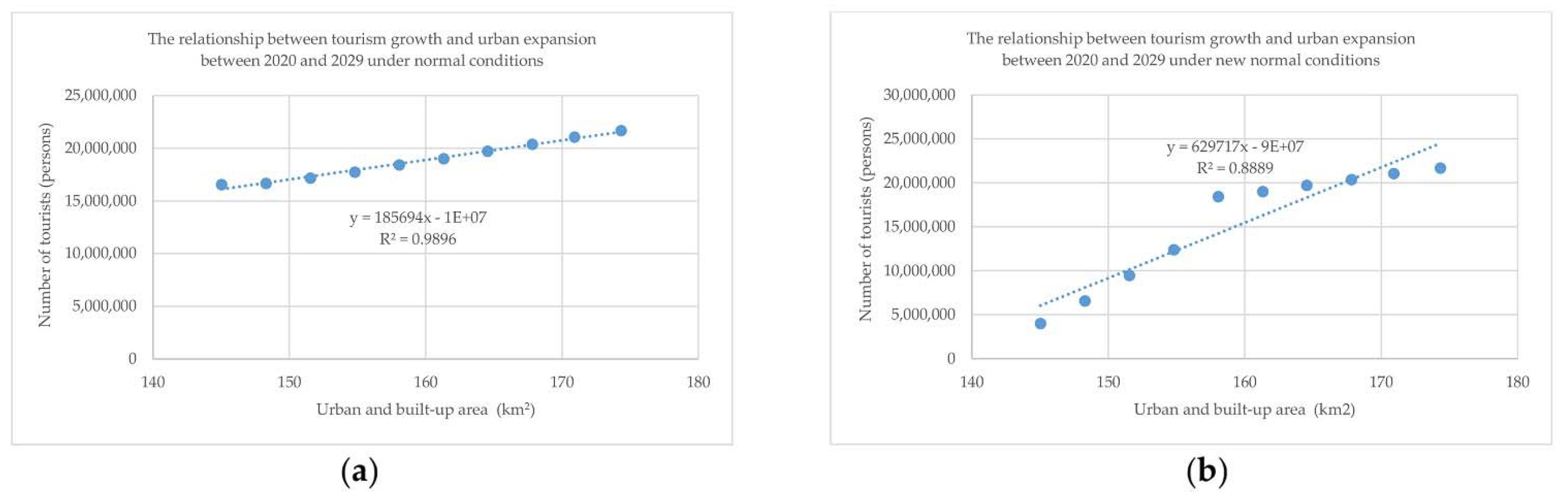
In addition, tourism growth under normal conditions shows a positive correlation with urban expansion in Phuket Island, with a high coefficient of determination (0.99) (Figure 14a). Tourism growth under new normal conditions is also positively correlated with urban expansion in Phuket Island, with a high coefficient of determination (0.89) (Figure 14b). These findings are in line with Rempis et al., who stated that urbanization, driven by either anthropogenic elements, such as population growth, or economic geography factors, contributes to the expansion of the extensive and intensive settlements [68].
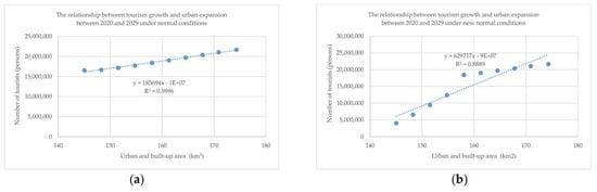
Figure 14.
Simple linear regression analysis between tourism growth and urban expansion in Phuket Island between 2020 and 2029: (a) normal condition; (b) new normal condition (COVID-19 pandemic).
Moreover, the increase in tourism led to the high resource demand of Phuket Island. Notably, water is a primary resource in many activities of daily life. A small island such as Phuket Island has limited water supply storage in summer, and water demand is high due to the high tourism in Phuket Island during this season. These findings agree with the results of Tokarchuk et al., who found that increasing tourist flows affect local economies and the lives of residents due to the construction of tourist facilities such as large hotels and huge recreational and commercial areas. This construction leads to the degradation of natural resources [69], for example, the littering of waste resulting from tourist traffic and decreased water resources due to excessive demand [70].
Recently, many projects have been initiated in Phuket Island to further its development, such as enhancing its status as a world-class tourism destination; making it a Smart city and MICE city; and building infrastructure (Phuket Airport expansion, light rail transit, and underpass), international schools, medical hub, international exhibition and conference centers, and shopping malls [71]. This continuous development will lead to the expected LULC change and tourism growth over a short period.
4.6.3. Water Demand for Agriculture and Forest Uses
The water demand for agriculture and forest uses was estimated based on the evapotranspiration coefficient and reference evapotranspiration [50]. The area of each agriculture and forest type between 2020 and 2029 and water demand are summarized in Table 23. According to the results, the total agriculture area will decrease from 185.76 km2 in 2020 to 167.57 km2 in 2029, with an average of 176.67 km2. Water demand for agriculture use will decrease from 264.84 million m3 in 2020 to 237.35 million m3 in 2029. The average water demand for agriculture use is 250.93 million m3. Furthermore, the total forest area will decrease from 124.49 km2 in 2020 to 113.00 km2 in 2029, with an average area of 118.78 km2. Water demand for forest use will decrease from 159.58 million m3 in 2020 to 142.74 million m3 in 2029. The average water demand for forest use is 151.10 million m3. This finding indicates that agriculture and forest land will decrease between 2020 and 2029.
Table 23.
Area of each agriculture and forest type and water demand between 2020 and 2029.
4.7. Water Balance Evaluation between 2020 and 2029
The annual and monthly water balance in terms of water surplus and deficit between 2020 and 2029 under dry and wet year scenarios in normal and new normal conditions (COVID-19 pandemic) was evaluated without and with the consideration of ecological water requirements for water resource management. For the evaluation of the monthly water balance, two essential data analyses were performed: monthly water supply without and with the consideration of ecological water requirements under dry and wet year scenarios and average monthly water demand in each category in normal and new normal conditions. The results are summarized in Table A4 and Table A5 in Appendix A.
4.7.1. Annual Water Balance without the Consideration of Ecological Water Requirements
The annual water balance evaluation results without the consideration of ecological water requirements under the two scenarios and conditions are reported in Table 24.
Table 24.
The annual water supply and demand balance evaluation without considering ecological water requirements between 2020 and 2029.
Under the dry year scenario, the annual water balance in the normal condition indicates a surplus in all years. The water surplus varies from 29.15 million m3 to 79.70 million m3, with an average water surplus of 54.12 million m3. In addition, the annual water balance in the new normal condition also indicates a surplus in all years. The water surplus varies from 43.38 million m3 to 79.70 million m3, with an average water surplus of 58.19 million m3.
Similarly, the annual water balance in the normal condition reveals a surplus in all years under the wet year scenario. The water surplus varies from 749.61 million m3 to 799.98 million m3, with an average water surplus of 774.89 million m3. In addition, the annual water balance in the new normal condition also indicates a surplus in all years under this scenario. The water surplus varies from 763.95 million m3 to 799.98 million m3, with an average water surplus of 778.97 million m3.
4.7.2. Monthly Water Balance without the Consideration of Ecological Water Requirements
Table 25 reports the results of the monthly water balance without the consideration of ecological water requirements in terms of surplus and deficit under the dry and wet year scenarios in the normal and new normal conditions between 2020 and 2029.
Table 25.
Monthly water supply and demand balance evaluation without consideration of ecological water requirements between 2020 and 2029.
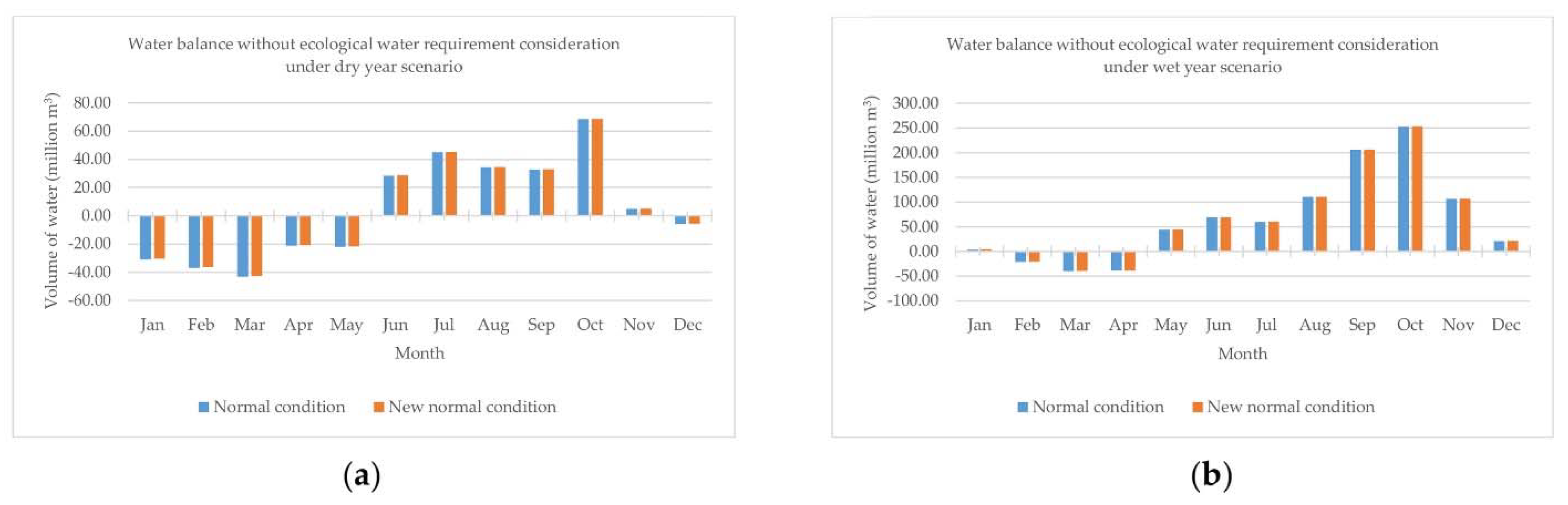
As indicated by the results in Table 25, under the dry year scenario in the normal condition, the monthly water balance reveals a deficit from December to May. It varies from −43.07 million m3 in March to −5.91 million m3 in December. However, the monthly water balance indicates a surplus from June to November, varying from 4.91 million m3 in November to 68.44 million m3 in October. Under the dry year scenario in the new normal condition, the monthly water balance indicates a deficit from December to May. It varies from −42.63 million m3 in March to −5.47 million m3 in December. However, the monthly water balance reveals a water surplus from June to November, varying from 5.22 million m3 in November to 68.77 million m3 in October.
On the contrary, the monthly water balance shows a deficit from February to April under the wet year scenario in the normal condition. It varies from −39.97 million m3 in March to −21.32 million m3 in February. However, the monthly water balance indicates a surplus from May to January, varying from 3.80 million m3 in January to 252.65 million m3 in October. In addition, the monthly water balance indicates a deficit from February to April under the wet year scenario in the new normal condition. It varies from −39.52 million m3 in March to −20.89 million m3 in February. However, the monthly water balance shows a surplus from May to January, varying from 4.26 million m3 in January to 252.97 million m3 in October.
Furthermore, Figure 15 displays the monthly water balance without the consideration of ecological water requirements in terms of surplus (positive) and deficit (negative) under the dry and wet year scenarios in the normal and new conditions.
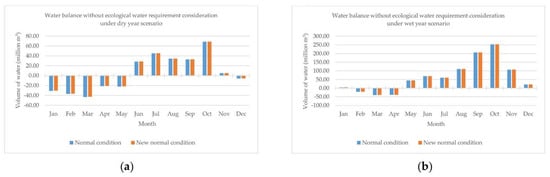
Figure 15.
Monthly water balance without the consideration of ecological water requirements under two scenarios in normal and new normal conditions: (a) dry year scenario; (b) wet year scenario.
4.7.3. Annual Water Balance with the Consideration of Ecological Water Requirements
Table 26 reports the evaluation results of the annual water balance in terms of water surplus or deficit between 2020 and 2029 with the consideration of ecological water requirements in the two different scenarios and conditions.
Table 26.
The annual water supply and demand balance evaluation with the consideration of ecological water requirements between 2020 and 2029.
Under the dry year scenario, the annual water balance in the normal condition indicates a deficit in all years. It varies from 67.94 million m3 to 118.49 million m3, with an average water deficit of 93.52 million m3. Similarly, the annual water balance in the new normal condition also shows a deficit in all years. It varies from 67.94 million m3 to 104.16 million m3, with an average water deficit of 89.45 million m3.
On the contrary, the annual water balance in the normal condition indicates a surplus in all years under the wet year scenario. It varies from 601.97 million m3 to 652.35 million m3, an average water surplus of 627.26 million m3. Similarly, the annual water balance in the new normal condition also shows a surplus in all years. It varies from 616.31 million m3 to 652.35 million m3, with an average water surplus of 631.33 million m3.
4.7.4. Monthly Water Balance with the Consideration of Ecological Water Requirements
Table 27 reports the monthly water balance with the consideration of ecological water requirements in terms of surplus and deficit under normal and new normal conditions between 2020 and 2029.
Table 27.
Monthly water supply and demand balance evaluation with the consideration of ecological water requirements between 2020 and 2029.
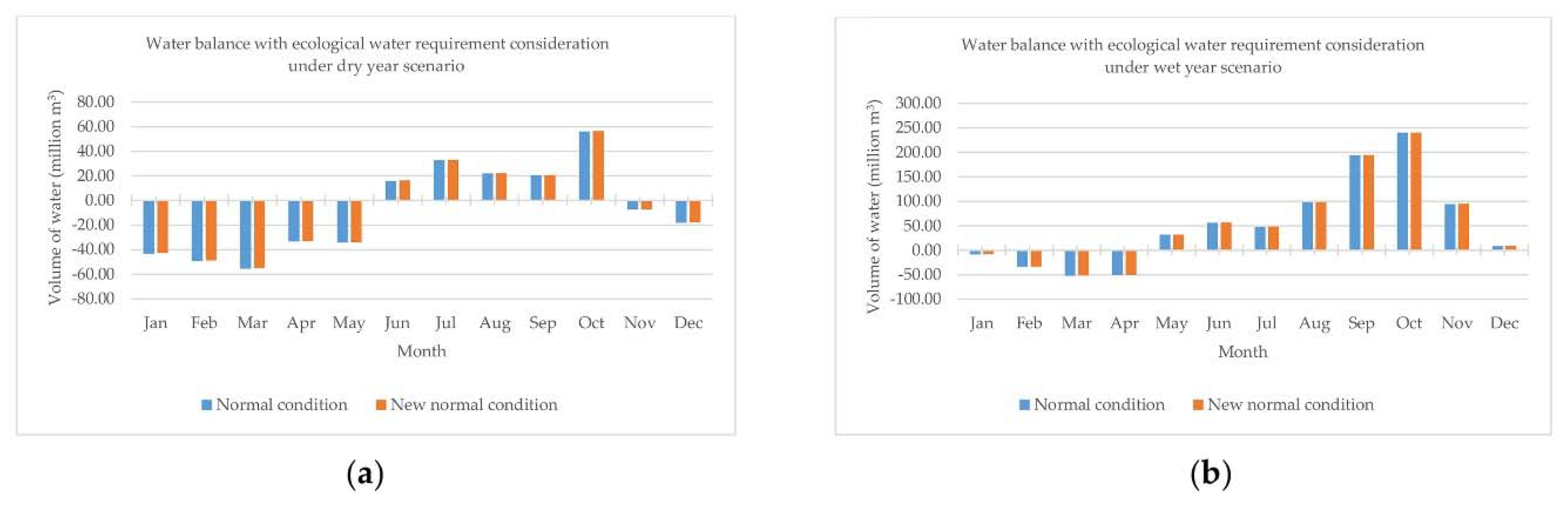
As indicated by the results in Table 27, under the dry year scenario in the normal condition, the monthly water balance shows a deficit from November to May. It varies from −55.37 million m3 in March to −7.39 million m3 in November. However, the monthly water balance indicates a surplus from June to October and varies from 16.03 million m3 in June to 56.14 million m3 in October. Under the dry year scenario in the new normal condition, the monthly water balance reveals a deficit from November to May. It varies from −54.93 million m3 in March to −7.08 million m3 in November. However, the monthly water balance in the same period indicates a surplus from June to October, varying from 16.37 million m3 in June to 56.47 million m3 in October.
On the contrary, the monthly water balance shows a deficit from January to April under the wet year scenario in the normal condition. It varies from −52.27 million m3 in March to −8.50 million m3 in January. However, the monthly water balance reveals a surplus from May to December, varying from 8.85 million m3 in December to 240.35 million m3 in October. In addition, the monthly water balance indicates a deficit from January to April under the wet year scenario in the new normal condition. It varies from −51.82 million m3 in March to −8.04 million m3 in January. However, the monthly water balance shows a surplus from May to December, varying from 9.28 million m3 in December to 240.67 million m3 in October.
Figure 16 displays the monthly water balance with the consideration of ecological water requirements in terms of surplus (positive) and deficit (negative) under the dry and wet year scenarios in the normal and new conditions.
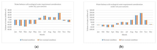
Figure 16.
Monthly water balance with consideration of ecological water requirements under two scenarios in normal and new normal conditions: (a) dry year scenario; (b) wet year scenario.
In summary, the annual water balance in Phuket Island without the consideration of ecological water requirements between 2020 and 2029 reveals a water surplus in all years under the dry and wet year scenarios in the normal and new normal conditions. Under the dry year scenario in the same period, the monthly water balance in Phuket Island without the consideration of ecological water requirements reveals a water deficit for six months (December–May) in the normal and new normal conditions. Under the wet year scenario, the monthly water balance in Phuket Island without the consideration of ecological water requirements indicates a water deficit for three months (February–April) in the normal and new normal conditions (see Figure 15).
On the contrary, when considering ecological water requirements, the annual water balance in Phuket Island between 2020 and 2029 shows a water deficit in all years under the dry year scenario in the normal and new normal conditions. However, under the wet year scenario for the same period, the annual water balance in Phuket Island indicates a water surplus in all years in the normal and new normal conditions. Under the dry year scenario, the monthly water balance in Phuket Island in the same period reveals a water deficit for seven months (November–May) in the normal and new normal conditions. Under the wet year scenario, the monthly water balance in Phuket Island shows a water deficit for four months (January–April) in the normal and new normal conditions (see Figure 16).
Accordingly, these findings indicate the effect of rainfall on the water balance in terms of deficit and surplus and imply the possibility of water scarcity in the future.
5. Conclusions
Land use and land cover assessment and change detection between 2014 and 2019 were successfully conducted using visual interpretation and a post-classification comparison change detection algorithm. The overall accuracy and Kappa hat coefficient of the LULC map in 2019 were more than 95%. Then, time-series LULC data between 2020 and 2029 were simulated using the CLUE-S model. These simulated LULC data provide realistic results that reflect expected trends. After that, to evaluate the water balance, the interpreted and simulated LULC data between 2019 and 2029 were used as the primary input to estimate water supply and demand. For the water supply assessment, annual and monthly water yields were successfully estimated using the SWAT model. In the calibration and validation periods under the dry and wet year conditions, the SWAT model performance ranged from good to very good according to statistical measurements, namely, the RMSE-observations standard deviation ratio, Nash–Sutcliffe efficiency, and percent bias. Furthermore, for the water demand assessment, three primary consumption activities—residential, tourist, and agriculture and forest use—were calculated under normal and new normal conditions using the water footprint basis. Finally, the annual and monthly water balance in terms of water surplus and deficit between 2020 and 2029 under dry and wet year scenarios in normal and new normal conditions was successfully evaluated without and with the consideration of ecological water requirements for water resource management. The annual water balance evaluation with the consideration of ecological water requirements revealed a water deficit every year under the dry year scenario in normal and new normal conditions. In addition, the monthly water balance indicated a water deficit in the summer every year, both without and with the consideration of ecological water requirements.
Consequently, it can be concluded that integrating remote sensing data (very high spatial resolution) with advanced geospatial models (CLUE-S model, SWAT model, and water footprint) can provide essential information about water supply, demand, and balance for water resources management, particular water scarcity, in Phuket Island in the future. This study’s conceptual framework and research workflows can assist government agencies in examining the water deficit in other areas, particularly the Northeast Region of Thailand, where agricultural drought frequently occurs.
Author Contributions
Conceptualization, S.O. and N.P.; methodology, S.O. and N.P.; software, N.P.; validation, S.O. and N.P.; formal analysis, S.O. and N.P.; investigation, S.O. and N.P.; data curation, N.P.; writing—original draft preparation, N.P.; writing—review and editing, S.O.; visualization, N.P.; supervision, S.O. All authors have read and agreed to the published version of the manuscript.
Funding
This research received no external funding.
Institutional Review Board Statement
Not applicable.
Informed Consent Statement
Not applicable.
Data Availability Statement
Not applicable.
Acknowledgments
The authors would like to thank the Suranaree University of Technology and Prince of Songkla University for supporting the facilities to undertake this research. The special thanks from the authors go to anonymous reviewers for their valuable comments and suggestions that improve our manuscript from various perspectives.
Conflicts of Interest
The authors declare no conflict of interest.
Appendix A
Table A1.
The evapotranspiration coefficient (Kc) of each agriculture and forest type.
Table A1.
The evapotranspiration coefficient (Kc) of each agriculture and forest type.
| No. | Agriculture and Forest Type | Evapotranspiration Coefficient (Kc) |
|---|---|---|
| 1 | Field crop | 0.6 |
| 2 | Paddy field | 0.6 |
| 3 | Para rubber trees | 1.0 |
| 4 | Evergreen forest | 1.0 |
| 5 | Mangrove forest | 1.0 |
| 6 | Scrub forest | 0.5 |
Note: The Kc values were obtained from Trisurat et al. [72].
Table A2.
The reference evapotranspiration under the Penman–Monteith method.
Table A2.
The reference evapotranspiration under the Penman–Monteith method.
| Station | ETo (mm/Day) | |||||||||||
|---|---|---|---|---|---|---|---|---|---|---|---|---|
| January | February | March | April | May | June | July | August | September | October | November | December | |
| Phuket | 4.29 | 4.62 | 4.55 | 4.34 | 3.84 | 3.81 | 3.78 | 3.98 | 3.43 | 3.53 | 3.65 | 3.83 |
| Phuket Airport | 4.04 | 4.37 | 4.58 | 4.36 | 3.93 | 3.93 | 3.92 | 3.78 | 3.52 | 3.19 | 3.32 | 3.67 |
| Average | 4.17 | 4.50 | 4.57 | 4.35 | 3.89 | 3.87 | 3.85 | 3.88 | 3.48 | 3.36 | 3.49 | 3.75 |
Note: The average values between Phuket and Phuket Airport stations from Royal Irrigation Department [73] were used in the analysis.
Table A3.
Annual water yield (dependent variable) and primary LULC types (independent variable) area in Phuket Island between 2020 and 2029.
Table A3.
Annual water yield (dependent variable) and primary LULC types (independent variable) area in Phuket Island between 2020 and 2029.
| Year | Water Yield (Million m3) | Area of LULC Type (km2) | ||||
|---|---|---|---|---|---|---|
| Dry Year Scenario | Wet Year Scenario | Urban and Built-Up Area | Perennial Tree and Orchard | Idle Land | Evergreen Forest | |
| 2020 | 505.01 | 1225.48 | 145.03 | 182.16 | 40.03 | 72.96 |
| 2021 | 505.73 | 1226.49 | 148.29 | 180.01 | 40.29 | 71.79 |
| 2022 | 506.34 | 1227.28 | 151.54 | 177.87 | 40.54 | 70.62 |
| 2023 | 507.41 | 1228.55 | 154.81 | 175.74 | 40.82 | 69.47 |
| 2024 | 508.28 | 1229.18 | 158.07 | 173.55 | 41.01 | 68.27 |
| 2025 | 510.06 | 1231.38 | 161.32 | 171.46 | 41.32 | 67.15 |
| 2026 | 517.83 | 1238.32 | 164.55 | 169.35 | 41.59 | 65.98 |
| 2027 | 519.55 | 1240.31 | 167.83 | 167.20 | 41.85 | 64.83 |
| 2028 | 520.22 | 1240.94 | 170.92 | 165.21 | 42.09 | 63.71 |
| 2029 | 521.79 | 1242.08 | 174.34 | 162.90 | 42.35 | 62.49 |
Table A4.
Monthly water supply without and with the consideration of ecological water requirements under dry and wet year scenarios between 2020 and 2029.
Table A4.
Monthly water supply without and with the consideration of ecological water requirements under dry and wet year scenarios between 2020 and 2029.
| Month | Water Supply without Ecological Water Requirement Consideration (Million m3) | Water Supply with Ecological Water Requirement Consideration (Million m3) | ||
|---|---|---|---|---|
| Dry year | Wet year | Dry year | Wet year | |
| January | 10.61 | 45.31 | −1.69 | 33.01 |
| February | 3.92 | 19.46 | −8.38 | 7.16 |
| March | 1.84 | 4.95 | −10.46 | −7.35 |
| April | 20.24 | 2.80 | 7.94 | −9.50 |
| May | 16.10 | 82.32 | 3.80 | 70.02 |
| June | 65.57 | 106.19 | 53.27 | 93.89 |
| July | 82.69 | 97.82 | 70.39 | 85.52 |
| August | 72.22 | 148.54 | 59.92 | 136.24 |
| September | 66.16 | 239.62 | 53.86 | 227.32 |
| October | 102.26 | 286.47 | 89.96 | 274.17 |
| November | 38.75 | 140.62 | 26.45 | 128.32 |
| December | 31.86 | 58.92 | 19.56 | 46.62 |
| Total | 512.22 | 1233.00 | 364.62 | 1085.40 |
| Average | 42.69 | 102.75 | 30.39 | 90.45 |
Table A5.
Average monthly water demand estimation of each category between 2020 and 2029 under normal and new normal conditions.
Table A5.
Average monthly water demand estimation of each category between 2020 and 2029 under normal and new normal conditions.
| Month | Type of Water Demand (Million m3) | ||||||
|---|---|---|---|---|---|---|---|
| Residential | Tourist | Agriculture Use | Forest Use | Total Water Demand | |||
| Normal | New Normal | Normal | New Normal | ||||
| January | 2.88 | 2.42 | 1.96 | 22.60 | 13.61 | 41.51 | 41.05 |
| February | 2.88 | 2.22 | 1.80 | 22.27 | 13.41 | 40.78 | 40.36 |
| March | 2.88 | 2.35 | 1.90 | 24.77 | 14.91 | 44.91 | 44.47 |
| April | 2.88 | 1.87 | 1.52 | 22.84 | 13.75 | 41.35 | 40.99 |
| May | 2.88 | 1.39 | 1.12 | 21.08 | 12.69 | 38.04 | 37.78 |
| June | 2.88 | 1.80 | 1.46 | 20.32 | 12.24 | 37.23 | 36.89 |
| July | 2.88 | 1.26 | 1.02 | 20.89 | 12.58 | 37.61 | 37.37 |
| August | 2.88 | 1.25 | 1.01 | 21.05 | 12.68 | 37.86 | 37.62 |
| September | 2.88 | 1.27 | 1.03 | 18.25 | 10.99 | 33.39 | 33.15 |
| October | 2.88 | 1.73 | 1.40 | 18.23 | 10.98 | 33.82 | 33.49 |
| November | 2.88 | 1.65 | 1.33 | 18.30 | 11.02 | 33.85 | 33.53 |
| December | 2.88 | 2.29 | 1.86 | 20.35 | 12.25 | 37.77 | 37.33 |
| Total | 34.58 | 21.49 | 17.42 | 250.93 | 151.10 | 458.11 | 454.03 |
References
- Information Technology and Communication Division, Phuket Provincial Office. Phuket Province Briefing 2010. Available online: http://123.242.171.10/descr/introduce/dataPK53/chapter4.pdf (accessed on 5 May 2019).
- Sakunboonpanich, Y. History of Modern City of Phuket from 1957 to 2007. Master’s Thesis, Thammasat University, Bangkok, Thailand, 2011. [Google Scholar]
- TAT Intelligence Center, Tourism Authority of Thailand. Tourist Arrivals to Phuket Island during 1993–2020. Available online: https://intelligencecenter.tat.or.th/articles/11859 (accessed on 10 February 2021).
- Economics Tourism and Sports Division, Ministry of Tourism and Sports. Domestic Tourism Statistics (Classify by Region and Province 2020). Available online: https://www.mots.go.th/more_news_new.php?cid=594 (accessed on 10 February 2021).
- Department of Provincial Administration, Ministry of Interior. Population of Phuket Province during 1993–2020. Available online: http://stat.bora.dopa.go.th/new_stat/webPage/statByYear.php (accessed on 25 January 2021).
- Kundu, S.; Khare, D.; Mondal, A. Past, present, and future land use changes and their impact on water balance. J. Environ. Manag. 2017, 197, 582–596. [Google Scholar] [CrossRef]
- Kifle, A.B.; Mengistu, T.G.; Stoffberg, G.H.; Tadesse, T. Climate change and population growth impacts on surface water supply and demand of Addis Ababa, Ethiopia. Clim. Risk Manag. 2017, 18, 21–33. [Google Scholar] [CrossRef]
- Reyes Perez, M.F. Water Supply and Demand Management in the Galápagos: A Case Study of Santa Cruz Island. Ph.D. Thesis, Delft University of Technology, Delft, The Netherlands, 2017. [Google Scholar]
- Li, T.; Yang, S.; Tan, M. Simulation and optimization of water supply and demand balance in Shenzhen: A system dynamics approach. J. Clean. Prod. 2019, 207, 882–893. [Google Scholar] [CrossRef]
- Liersch, S.; Fournet, S.; Koch, H.; Djibo, A.G.; Reinhardt, J.; Kortlandt, J.; Van Weert, F.; Seidou, O.; Klop, E.; Baker, C.; et al. Water resources planning in the Upper Niger River basin: Are their gaps between water demand and supply. J. Hydrol. Reg. Stud. 2019, 21, 176–194. [Google Scholar] [CrossRef]
- Charupongsopon, W. Potential of Water Resources in Changwat Phuket. Master’s Thesis, Chiang Mai University, Chiang Mai, Thailand, 1990. [Google Scholar]
- Leelawattanagoon, P. Streamflow Characteristics of Phuket Island. Master’s Thesis, Kasetsart University, Bangkok, Thailand, 2003. [Google Scholar]
- Thepnuan, P. A System Dynamics Model of Tourism Development Carrying Capacity of water Resource in Changwat Phuket. Master’s Thesis, Prince of Songkla University, Songkhla, Thailand, 2007. [Google Scholar]
- Vongtanaboon, S.; Boochabun, K.; Meunpon, R.; Sriyaporn, C. Water Quantity Analysis in Phuket Province; Phuket Rajabhat University: Phuket, Thailand, 2010. [Google Scholar]
- Sma-air, S. Analysis of Surface-Water Resource Amount for Water Management in Phuket Province, Thailand. Master’s Thesis, Prince of Songkla University, Songkhla, Thailand, 2012. [Google Scholar]
- Hanuphab, T. Water Budget Assessment in Phuket Province. Master’s Thesis, Prince of Songkla University, Songkhla, Thailand, 2013. [Google Scholar]
- Suwanprasit, C.; Puangkeaw, N.; Srichai, N. Water balance of Phuket province. J. Remote Sens. GIS Assoc. Thail. 2013, 14, 1–8. [Google Scholar]
- Prince of Songkla University, Phuket Campus. A Summary of the Water Situation. Available online: http://smartwaterphuket.com/#report (accessed on 12 April 2019).
- Information Technology and Communication Division, Phuket Provincial Office. Phuket Province Briefing 2012. Available online: http://123.242.171.10/descr/introduce/dataPK55.pdf (accessed on 5 May 2019).
- Thai Meteorological Department. Agricultural Meteorology to Know for Phuket; Thai Meteorological Department: Bangkok, Thailand, 2017. [Google Scholar]
- Boonchoo, K. Geospatial Models for Land Use and Land Cover Prediction and Deforestation Vulnerability Analysis in Phuket Island, Thailand. Ph.D. Thesis, Suranaree University of Technology, Nakhon Ratchasima, Thailand, 2015. [Google Scholar]
- Lillesand, T.M.; Kiefer, R.W.; Chipman, J.W. Remote Sensing and Image Interpretation, 5th ed.; John Wiley: New York, NY, USA, 2004. [Google Scholar]
- Lillesand, T.M.; Kiefer, R.W.; Chipman, J.W. Remote Sensing and Image Interpretation, 7th ed.; John Wiley: New York, NY, USA, 2015. [Google Scholar]
- Congalton, R.G.; Green, K. Assessing the Accuracy of Remotely Sensed Data: Principles and Practices, 2nd ed.; CRC Press: Boca Raton, FL, USA, 2009. [Google Scholar]
- Coppin, P.; Jonckheere, I.; Nackaerts, K.; Muys, B.; Lambin, E. Digital change detection methods in ecosystem monitoring: A review. Int. J. Remote Sens. 2004, 25, 1565–1596. [Google Scholar] [CrossRef]
- Jensen, J.R. Introductory Digital Image Processing: A Remote Sensing Perspective, 4th ed.; Pearson Education: Glenview, IL, USA, 2015. [Google Scholar]
- Cabral, P.; Zamyatin, A. Markov processes in modeling land use and land cover changes in Sintra-Cascais, Portugal. Dyna 2009, 76, 191–198. [Google Scholar]
- Ongsomwang, S.; Boonchoo, K. Integration of Geospatial Models for the Allocation of Deforestation Hotspots and Forest Protection Units. Suranaree J. Sci. Technol. 2016, 23, 283–307. [Google Scholar]
- Verburg, P.H.; de Koning, G.H.J.; Kok, K.; Veldkamp, A.; Bouma, J. A spatial explicit allocation procedure for modeling the pattern of land-use change based upon actual land use. Ecol. Model. 1999, 116, 45–61. [Google Scholar] [CrossRef]
- Verburg, P.H.; Soepboer, W.; Veldkamp, A.; Limpiada, R.; Espaldon, M.V.; Mastura, S. Modeling the Spatial Dynamics of Regional Land Use: The CLUE-S Model. Environ. Manag. 2002, 30, 391–405. [Google Scholar] [CrossRef]
- Verburg, P.H.; Overmars, K.P. Dynamic Simulation of Land-Use Change Trajectories with the CLUE-S Model. In Modelling Land-Use Change: Progress and Applications; Koomen, E., Stillwell, J., Bakema, A., Scholten, H.J., Eds.; Springer: Dordrecht, The Netherlands, 2007; pp. 321–337. [Google Scholar]
- Arnold, J.G.; Fohrer, N. SWAT2000: Current capabilities and research opportunities in applied watershed modeling. Hydrol. Process. 2005, 19, 563–572. [Google Scholar] [CrossRef]
- Gassman, P.W.; Reyes, M.R.; Green, C.H.; Arnold, J.G. The Soil and Water Assessment Tool: Historical Development, Applications, and Future Research Directions. Trans. ASABE 2007, 50, 1211–1250. [Google Scholar] [CrossRef] [Green Version]
- Douglas-Mankin, K.; Srinivasan, R.; Arnold, J. Soil and Water Assessment Tool (SWAT) Model: Current Developments and Applications. Trans. ASABE 2010, 53, 1423–1431. [Google Scholar] [CrossRef]
- Kunto, S.; Ongsomwang, S. Optimum parameters for water runoff estimating in Huay Tung Lung watershed of Mun basin, Ubon Ratchathani province. In Proceedings of the 1st Geoinformatics Conference for Graduate Students and Young Researchers 2013 (1st GI-GRAD 2013), Nakhon Ratchasima, Thailand, 19–21 June 2013. [Google Scholar]
- Sisay, E.; Halefom, A.; Khare, D.; Singh, L.; Meshesha, T. Hydrological modeling of an ungauged urban watershed using SWAT model. Model. Earth Syst. Environ. 2017, 3, 693–702. [Google Scholar] [CrossRef]
- Schilling, K.; Jha, M.; Zhang, Y.-K.; Gassman, P.; Wolter, C. Impact of Land Use and Land Cover Change on the Water Balance of a Large Agricultural Watershed: Historical Effects and Future Directions. Water Resour. Res. 2008, 44, 1–12. [Google Scholar] [CrossRef]
- Arnold, J.G.; Moriasi, D.N.; Gassman, P.W.; Abbaspour, K.C.; White, M.J.; Srinivasan, R.; Santhi, C.; Harmel, R.D.; Van Griensven, A.; Van Liew, M.W.; et al. Swat: Model Use, Calibration, and Validation. Trans. ASABE 2012, 55, 1491–1508. [Google Scholar] [CrossRef]
- Leta, O.T.; El-Kadi, A.I.; Dulai, H.; Ghazal, K.A. Assessment of climate change impacts on water balance components of Heeia watershed in Hawaii. J. Hydrol. Reg. Stud. 2016, 8, 182–197. [Google Scholar] [CrossRef] [Green Version]
- Veettil, A.V.; Mishra, A.K. Water security assessment using blue and green water footprint concepts. J. Hydrol. 2016, 542, 589–602. [Google Scholar] [CrossRef]
- Ayivi, F.; Jha, M.K. Estimation of water balance and water yield in the Reedy Fork-Buffalo Creek Watershed in North Carolina using SWAT. Int. Soil Water Conserv. Res. 2018, 6, 203–213. [Google Scholar] [CrossRef]
- Luan, X.; Wu, P.; Sun, S.; Wang, Y.; Gao, X. Quantitative study of the crop production water footprint using the SWAT model. Ecol. Indic. 2018, 89, 1–10. [Google Scholar] [CrossRef]
- Osei, M.A.; Amekudzi, L.K.; Wemegah, D.D.; Preko, K.; Gyawu, E.S.; Obiri-Danso, K. The impact of climate and land-use changes on the hydrological processes of Owabi catchment from SWAT analysis. J. Hydrol. Reg. Stud. 2019, 25, 100620. [Google Scholar] [CrossRef]
- Legates, D.; McCabe, G. Evaluating the Use of “Goodness-of-Fit” Measures in Hydrologic and Hydro climatic Model Validation. Water Resour. Res. 1999, 35, 233–241. [Google Scholar] [CrossRef]
- Nash, J.E.; Sutcliffe, J.V. River flow forecasting through conceptual models part I—A discussion of principles. J. Hydrol. 1970, 10, 282–290. [Google Scholar] [CrossRef]
- Gupta, H.V.; Sorooshian, S.; Yapo, P.O. Status of Automatic Calibration for Hydrologic Models: Comparison with Multilevel Expert Calibration. J. Hydrol. Eng. 1999, 4, 135–143. [Google Scholar] [CrossRef]
- Moriasi, D.N.; Arnold, J.G.; Van Liew, M.W.; Bingner, R.L.; Harmel, R.D.; Veith, T.L. Model Evaluation Guidelines for Systematic Quantification of Accuracy in Watershed Simulations. Trans. ASABE 2007, 50, 885–900. [Google Scholar] [CrossRef]
- Royal Irrigation Department. Work Manual: Volume 8/16 Assessment of Water Use in Various Activities; Royal Irrigation Department: Bangkok, Thailand, 2011. [Google Scholar]
- Srichai, N.; Kuayrakan, S.; Suwanprasit, C. Water Use and Water Demand Modeling for Hotel and Tourism Business, Patong, Phuket Province. Songklanakarin J. Soc. Sci. Humanit. 2016, 22, 255–292. [Google Scholar]
- Allen, R.G.; Pereira, L.S.; Raes, D.; Smith, M. Crop Evapotranspiration-Guidelines for Computing Crop Water Requirements—FAO Irrigation and Drainage Paper 56; Food and Agriculture Organization: Rome, Italy, 1998. [Google Scholar]
- Southern Region Irrigation Hydrology Center, Royal Irrigation Department. The Monitoring Low Water Criteria Using Flow Duration Curve; Bureau of Water Management and Hydrology Royal Irrigation Department: Bangkok, Thailand, 2021. [Google Scholar]
- Fitzpatrick-Lins, K. Comparison of sampling procedures and data analysis for a land-use and land cover map. Photogramm. Eng. Remote Sens. 1981, 47, 343–351. [Google Scholar]
- Anderson, J.R.; Hardy, E.E.; Roach, J.T.; Witmer, R.E. A Land Use and Land Cover Classification System for Use with Remote Sensor Data; Geological Survey of United States: Washington, DC, USA, 1976. [Google Scholar]
- Naikoo, M.W.; Rihan, M.; Ishtiaque, M. Analyses of land use land cover (LULC) change and built-up expansion in the suburb of a metropolitan city: Spatio-temporal analysis of Delhi NCR using Landsat datasets. J. Urban Manag. 2020, 9, 347–359. [Google Scholar] [CrossRef]
- Imran, H.M.; Hossain, A.; Islam, A.K.M.S.; Rahman, A.; Bhuiyan, M.A.E.; Paul, S.; Alam, A. Impact of Land Cover Changes on Land Surface Temperature and Human Thermal Comfort in Dhaka City of Bangladesh. Earth Syst. Environ. 2021, 5, 667–693. [Google Scholar] [CrossRef]
- Hosmer, D.; Lemeshow, S.; Sturdivant, R. Applied Logistic Regression, 3rd ed.; John Wiley & Sons: Hoboken, NJ, USA, 2013. [Google Scholar]
- Van Asselen, S.; Verburg, P. Land cover change or land-use intensification: Simulating land system change with a global-scale land change model. Glob. Chang. Biol. 2013, 19, 3648–3667. [Google Scholar] [CrossRef]
- Liu, M.; Wang, Y.; Li, D.; Xia, B. Dyna-CLUE Model Improvement Based on Exponential Smoothing Method and Land Use Dynamic Simulation. In Geo-Informatics in Resource Management and Sustainable Ecosystem; Bian, F., Xie, Y., Cui, X., Zeng, Y., Eds.; Springer: Berlin/Heidelberg, Germany, 2013; pp. 266–277. [Google Scholar]
- Xu, L.; Li, Z.; Song, H.; Yin, H. Land-Use Planning for Urban Sprawl Based on the CLUE-S Model: A Case Study of Guangzhou, China. Entropy 2013, 15, 3490–3506. [Google Scholar] [CrossRef]
- Tolk, J.A. Plant available soil water. In Encyclopedia of Water Science; Stewart, B.A., Howell, T.A., Eds.; Marcel Dekker: New York, NY, USA, 2003; pp. 669–672. [Google Scholar]
- Opere, A.; Okello, B. Hydrologic analysis for river Nyando using SWAT. Hydrol. Earth Syst. Sci. Discuss. 2011, 8, 1765–1797. [Google Scholar]
- Ongsomwang, S.; Kunto, S. Impact of Land Use Change on Water Runoff A Case Study of Huay Tung Lung Watershed in the Mun Basin. J. Remote Sens. GIS Assoc. Thail. 2013, 14, 1–7. [Google Scholar]
- Hu, S.; Fan, Y.; Zhang, T. Assessing the Effect of Land Use Change on Surface Runoff in a Rapidly Urbanized City: A Case Study of the Central Area of Beijing. Land 2020, 9, 17. [Google Scholar] [CrossRef] [Green Version]
- Puno, R.C.C.; Puno, G.R.; Talisay, B.A.M. Hydrologic responses of watershed assessment to land cover and climate change using soil and water assessment tool model. Glob. J. Environ. Sci. Manag. 2019, 5, 71–82. [Google Scholar]
- Boretti, A.; Rosa, L. Reassessing the projections of the World Water Development Report. Nat. Partn. J. Clean Water 2019, 2, 1–6. [Google Scholar] [CrossRef]
- Wijitkosum, S.; Sriburi, T. Impact of Urban Expansion on Water Demand: The case study of Nakhon Ratchasima city, Lam Ta Kong Watershed. Nakhara J. Environ. Des. Plan. 2008, 4, 69–88. [Google Scholar]
- Liu, W.; Zhao, M.; Cai, Y.; Wang, R.; Lu, W. Synergetic Relationship between Urban and Rural Water Poverty: Evidence from Northwest China. Int. J. Environ. Res. Public Health 2019, 16, 1647. [Google Scholar] [CrossRef] [Green Version]
- Rempis, N.; Alexandrakis, G.; Kampanis, N. Urbanization and coastal effects in Agia Pelagia, Crete Island. In Proceedings of the 20th EGU General Assembly, EGU2018, Vienna, Austria, 7–12 April 2019. [Google Scholar]
- Tokarchuk, O.; Gabriele, R.; Maurer, O. Development of city tourism and well-being of urban residents: A case of German Magic Cities. Tour. Econ. 2017, 23, 343–359. [Google Scholar] [CrossRef]
- Troanca, D. The impact of tourism development on urban environment. Stud. Bus. Econ. 2012, 7, 160–164. [Google Scholar]
- Information Technology and Communication Division, Phuket Provincial Office. Phuket Province Briefing 2016. Available online: https://www.phuket.go.th/webpk/file_data/intropk/dataPK59.pdf (accessed on 5 May 2019).
- Trisurat, Y.; Aekakkararungroj, A.; Johnston, J.M.; Nuon, V.; Phan, N. Basin-Wide Assessments of Climate Change Impacts on Water and Water-Related Resources and Sector in Lower Mekong Basin; Mekong River Commission Planning Division: Phnom Penh, Cambodia, 2017. [Google Scholar]
- Royal Irrigation Department. Crop Water Requirement, Reference Crop Evapotranspiration and Crop Coefficient Handbook; Royal Irrigation Department: Bangkok, Thailand, 2011. [Google Scholar]

Publisher’s Note: MDPI stays neutral with regard to jurisdictional claims in published maps and institutional affiliations. |
© 2021 by the authors. Licensee MDPI, Basel, Switzerland. This article is an open access article distributed under the terms and conditions of the Creative Commons Attribution (CC BY) license (https://creativecommons.org/licenses/by/4.0/).