Public Transportation Operational Health Assessment Based on Multi-Source Data

Featured Application

This work is based on a complex urban transit environment and uses a machine learning approach based on the integrated analysis of multiple sources of data for the analysis and determination of factors influencing transit health levels. The results of the study provide a feasible application of the method in the field of urban transit data analysis.

Abstract

In order to solve the problem of inefficient long-term operation of urban public transport vehicles and the difficulty of finding the cause of the disease, a new analysis idea was designed using machine learning methods. This study aimed to provide a rapid, accurate, and convenient solution model and algorithm to address the drawbacks of traditional analysis tools that are incapable of handling multiple sources of public transport data. Based on a full process analysis of the bus operation status, the influencing factors and calculation methods were defined. Afterwards, the calculation results were used to construct a training set with a Random Forest regression model to obtain the weight ranking of different influencing factors. The results of the simulation validation proved that the model can use the basic data of bus operation to quickly find out the primary factors affecting the operation condition and pinpoint to the bottleneck interval. The method has high accuracy and feasibility. It can be universally applied to the analysis of regular bus scenarios to provide strong decision support for the operation level.

1. Introduction

The development goal of modern transportation is to reasonably meet transportation needs, optimize resource utilization, improve environmental quality, promote social harmony, enhance safety, and achieve the benign development of society, economy, environment, and transportation. With the increasing urbanization and rapid socio-economic development in China, the number of urban population and car ownership has increased dramatically, and urban traffic problems have become increasingly prominent. In order to alleviate the adverse effects of these problems, the vigorous development of public transportation is widely considered to be a very effective means [1].

However, the deteriorating conditions of public transport operations have led to various “public transport diseases”, especially the increase in travel time of travelers during peak hours, which in turn has led to the lack of attraction of the public transport system and the low share of public transport trips. The 2018 Shanghai Comprehensive Transportation Annual Report [2] shows that in 2018, 9.692 million passenger trips/day were carried by rail transit in Shanghai, up 4.0% year-on-year, accounting for 54.0% of urban passenger traffic; 6.03 million passenger trips/day were carried by public buses (electric), down 6.2% year-on-year, accounting for 33.6%. The above data show that low efficiency and low reliability seriously limit the long-term development of public transport systems. At the same time, the improvement of the public transportation network is accompanied by increasingly close connections with other social systems, and the complexity of various types of data has increased significantly beyond the processing capacity of traditional data analysis tools. Therefore, the use of machine learning methods based on integrated analysis of multi-source data to definite, evaluate, and cause analysis of the factors affecting the health of urban bus operation have become urgent research.

At present, domestic and international research on public transport operation diagnosis mainly focuses on the construction of diagnostic index systems and the selection of diagnostic methods. Peng chose measure departure time, running time, and arrival interval reliability as evaluation indicators. Afterwards, a comprehensive evaluation system for bus service reliability was constructed and applied to the actual evaluation in the context of the routes [3]. Liu integrated four indicators, including measures of journey time consistency, into a valid composite indicator set. The panel data analysis was used to provide confidence intervals for the composite indicator values for each direction of travel for each bus route to quickly determine the operating conditions of the route [4]. Wei established a public transport service evaluation index system with convenience, reliability, and comfort as the objectives [5]. Wen established an intercity bus travel satisfaction evaluation system based on improved hierarchical analysis and fuzzy comprehensive evaluation methods to examine the economy, reliability, convenience, comfort, and accessibility of the bus system, respectively [6].

The usual approach to the study of health diagnostic methods is to calculate weights based on a system of indicators and then use the results of the calculations to measure them. The weight determination methods include fuzzy comprehensive evaluation method [7,8], hierarchical analysis method and expert decision method [9,10], DEA method [11], and entropy value method [12]. Among them, the fuzzy comprehensive evaluation method is a good method for solving fuzzy, difficult to quantify non-deterministic problems and is more adaptable for solving practical problems. However, the selection of its parameters such as the determination of fuzzy matrix and the selection of affiliation degree is difficult and too subjective. Hierarchical analysis and expert decision method are also more subjective evaluation methods, which depend on the evaluator’s knowledge of the problem and are not suitable for use alone. DEA (Data Envelopment Analysis) is a quantitative analysis method for evaluating the relative effectiveness of comparable units of the same type based on multiple input indicators and multiple output indicators. The DEA method is actually a linear programming model to determine whether the same type of decision units with similar roles are on the production frontier. The entropy method is an objective evaluation method that can make full use of the available data and determine the index weights according to the volatility of the data [13]. Zhang used fuzzy set theory as the basis by investigating passengers’ perceptions. A fuzzy weighted average of all indicators was then adopted as a way to evaluate the state of public transport [14]. Xin proposed a GIS-based fuzzy clustering analysis method for the service level of public transport systems. Combining qualitative and quantitative evaluations, the system analysis of public transport service level was completed [15]. Using a three-parameter model and an operational state space model, Fan completed the evaluation of the level of bus service by region and state. The quantitative criteria established by this method are based on a three-dimensional state space and are more objective [16]. Ouyang completed the construction of a multi-factor vehicle driving condition recognition model based on a neural network approach [17]. Daniel completed the construction of a multi-factor vehicle driving state discrimination model based on the LVQ model, which contains 26 factors [18].

Although many scholars have made many research achievements in the areas of multi-source data fusion methods, bus operation evaluation, and health diagnosis methods, there are still some poorly considered aspects. Firstly, existing research on bus operational diagnosis lacks an effective means of classifying operational health levels. Non-artificial intelligence methods require the calculation of all bus routes one by one, which takes a lot of time and is highly subjective [19,20]. Secondly, many studies on the evaluation of bus operating conditions only give values for evaluation indicators rather than diagnostic criteria. For bus management and operators, it is not enough to identify the problem. They are more interested in what the cause of the problem is and how to solve it. Therefore, it is important to find and use convenient and effective machine learning methods to conduct integrated research on condition evaluation and cause analysis of bus operations. The machine learning algorithms used in this study belong to supervised learning. It is necessary to first construct a training set, select a suitable model from the existing training samples, and make a judgment on the health of the bus operation [21,22].

Among commonly used supervised learning machine learning algorithms, the SVM (Data Envelopment Analysis) algorithm is generally suitable for binary classification problems [23,24], and the Naive Bayes algorithm is suitable for datasets with mutually independent feature values [25]. The Decision Tree algorithm [26,27], the K-Nearest Neighbors algorithm [28], and the Random Forest algorithm [29,30] are all more effective methods for the dataset under study. The K-Nearest Neighbors is easy to understand, simple and effective, relatively insensitive to outliers, and capable of solving both binary classification and multi-classification problems. The Decision Tree is useful for helping to make decisions under uncertainty, allowing data scientists to traverse forward and backward computational paths to help make the best decisions and judgments; and the Decision Tree is insensitive to missing values and outliers, helping to save time in data processing, and is an effective method for classifying the health status of bus operations. The Random Forest is a collection of decision trees that are fast to train and can be used to rank the importance of variables and analyze the key causal factors affecting the health of public transport operations. In this paper, we use the Decision Tree and K-Nearest Neighbors to diagnose the health of bus operation, compare and analyze the effectiveness of the two methods, and select the optimal algorithm. Then, we output the key causal factors of bus operation based on Random Forest algorithm. This study was based entirely on bus operation data to find the problem. It used a diagnostic reasoning machine to solve the problem health diagnosis and cause analysis in an integrated way, improving the shortcomings of previous studies where only the symptoms of the disease are known, but not the cause.

2. Concept Definition and Calculation

2.1. Factors Influencing the Health of Public Transportation Operations

The public transportation operation system is a complex and comprehensive system formed by the interaction of passengers, vehicles, road network, and environment. Different factors influence each other, and they are subject to mutual constraints. At the same time, it is also subject to the interference of other contingent uncertainties. The stability and efficiency of public transportation operation is also characterized by randomness. The diagram of the public transport operation process is shown in Figure 1.

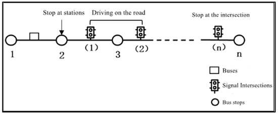
Figure 1. Diagram of bus operation process.

The scope of this paper is limited to the single-route bus operation level, analyzing the whole process of vehicles starting from the first station, traveling on the roadway, stopping at stations and intersections, and finally arriving at the last station; thus, it does not involve the bus network structure and station arrangement, bus route repetition number, non-linear coefficient, and other influencing factors at the bus planning level. Only the road delays, cross delays, and station delays in bus operation are diagnosed and analyzed, and improvement suggestions are made for different types of key influencing factors.

(1) Road delays

In the process of bus operation, the travel time of the vehicle running on the road section accounts for a large part of the full running time of the bus vehicle. Roadway congestion can lead to an increase in travel time for bus operations. During bus operations, especially during peak periods, the traffic volume on the roadway increases significantly, and traffic will run slower, affecting the speed of bus operations; therefore, road delays are a major influence on the health of bus operations.

(2) Intersection waiting time

Bus vehicles in the process of operation, the intersection encounter red light queue, and the time generated by the delay are also an important factor affecting the health status of public transport operations, and through the intersection of the time generated by the proportion of delay compared to the delay generated by roadway congestion, the difference is not large. The longer the bus waits in line at the intersection, the longer the delay will be and the worse the health of the bus operation will be. If the delay of bus vehicles is not reduced through signalized intersections, bus operational health cannot be improved effectively.

(3) Stopping time

Bus stopping process refers to the bus vehicle from slowly decelerating into the bus station, and then slowly accelerating away from the bus station into the process of traffic. The characteristics of public transport itself refer to the following: it is decided that the bus at each stop to have a slowdown and stop and speed up the process of leaving. The number of passengers boarding and alighting from the station, whether or not the ticket is automatic, etc., will affect the stopping time, which in turn affects the overall health of the bus operation. The more there are stops, the higher the passenger volume will be, and the longer the stop time will be.

(4) Other factors

Driver driving behavior, weather conditions, and other factors will also affect the bus running conditions. Different drivers have different personalities and are familiar with different degrees of bus vehicles, which can also affect the vehicle running delays; different weather conditions and different bus vehicle performance may also affect the bus operation. As the 101 bus for a fixed departure interval, thus the impact of the departure interval on the bus operation is not considered in this paper.

2.2. Definition of Eigenvalues of Influencing Factors

To quantify the impact of different influencing factors on the health of bus operations, it is necessary to first calculate the characteristic values of the influencing factors. This study defines and quantifies the main factors affecting bus operation including roadway delays, intersection delays, and stop time delays based on existing road network conditions from existing data.

(1) Station delay

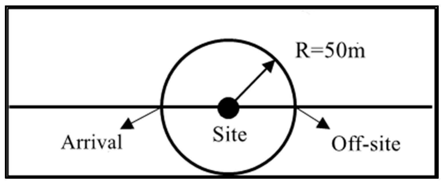
Station delay is directly expressed by the stopping time, which refers to the time from when the bus vehicle slows down to enter the platform to when the bus leaves the platform completely, as shown in Figure 2.

$$T_s=T_{sl}-T_{sa}$$

(1)

Figure 2. Station delay diagram.

In Formula (1), $T_s$ represents the stopping time. $T_{sl}$ refers to the moment when the bus leaves the station. $T_{sa}$ refers to the moment when the bus arrives at the station. In the case of bus vehicle positioning data, within 50 m from the station and the speed is less than 8 m/s marked as a stop, if the minimum speed within 50 m of the station is greater than 8 m/s, marked stopping time is 0.

(2) Cross delay

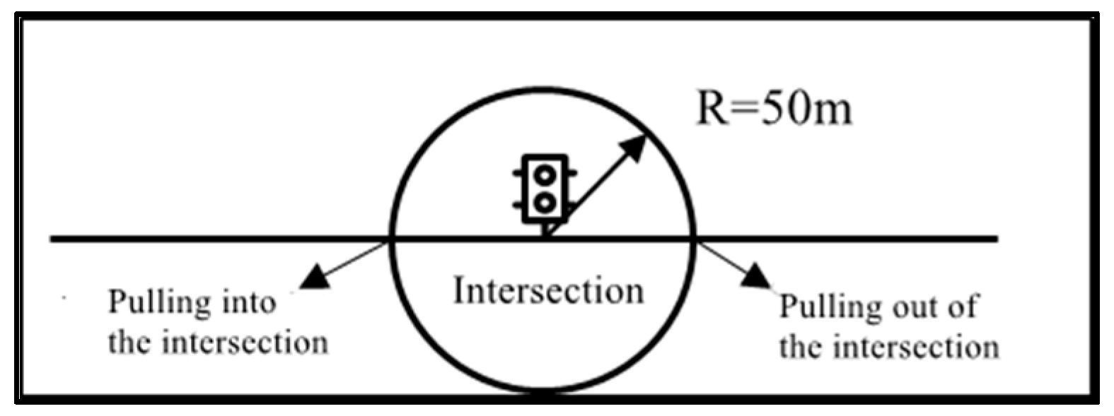
Due to data limitations, only bus vehicle operation data were obtained, and this study was not able to calculate delays in combination with intersection traffic, which was calculated directly from bus operation GPS data. Cross delay refers to the delay time from the time the bus enters the intersection and slows down until the bus leaves the intersection completely [31], as shown in Figure 3, Cross delay diagram.

$$T_c=(T_{cl}-T_{ca})-\frac{2R}{v_f}$$

(2)

Figure 3. Cross delay diagram.

In Formula (2), $T_c$ represents the cross delay. $T_{cl}$ refers to the time the bus leaves the intersection. $R$ refers to the intersection impact range, urban road intersection sight distance taken 30 m, plus the intersection center to the parking line between the distance of about 20 m. Therefore, take the intersection center point before and after 50 m as the intersection impact range. $v_f$ is the free flow speed, equal to the highest roadway speed. The cross delay is equal to the difference between the travel time for 50 m before and after each intersection and the time taken to travel the same distance at free flow speed.

(3) Road Delay

Road delay refers to the delay time from the bus traveling on the segment between intersections, as shown in Figure 4.

$$T_l=(T_{ca(i)}-T_{cl(i-1)})-\frac{l}{v_f}-T_s$$

(3)

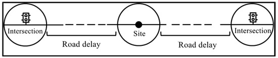
Figure 4. Road delay diagram.

In Formula (3), $T_l$ refers to the road delay. $T_{ca\left(i\right)}$ refers to the time in leaving the area of influence of the intersection. $T_{cl\left(i-1\right)}$ refers to the time the bus leaves the $\left(\mathrm{i}-1\right)$ intersection. $l$ refers to the actual distance the bus runs between two intersections. $T_s$ refers to the station delay. For bus operations, a bus stop may be passed between two intersections. Hence, the station delay needs to be subtracted from the real road delay.

(4) Weather factors

In this paper, we studied the data of bus operation from 21 November to 25 November 2016 with weather conditions as shown in Table 1 below. The weather conditions varied during the five days. Separate values are assigned for different weather.

Table 1. Weather conditions.

Date	Weather	Assignment
21-11-2016	Cloudy	2
22-11-2016	Light rain	4
23-11-2016	Medium Rain	4
24-11-2016	Light rain	3
25-11-2016	Sunny	1

(5) Driver driving behavior factors

Route 101 was assigned 18 vehicles from 21 November to 25 November according to the mapping relationship between license plates and routes. The license plates were assigned values 1–18, respectively, as a way to study the impact of different drivers’ driving behaviors on the health of bus operation.

Driver driving behavior and other vehicle factors will also affect the bus running conditions. Different weather conditions may also affect the bus operation. As the 101 bus for a fixed departure interval, the impact of the departure interval on the bus operation is not considered.

2.3. Calculation of the Eigenvalues of Influencing Factors

(1) Calculation of characteristic values

In this paper, Foshan Bus No. 101, whose operation is located in the urban area and the quality of data collection is relatively good, was selected as an example to calculate the station delay, cross delay and road delay of Bus No. 101 in the upward direction from 21 November to 25 November 2016, respectively.

The total length of Foshan Bus 101 is 12.86 km, via 27 stations and 19 signal intersections. Python software was used to calculate the delays for all trips issued on Foshan Bus 101 during the five days from 21 November to 25 November 2016. The trips were numbered in order from north to south. Taking one trip as an example, the statistical tables are shown in Table 2, Table 3 and Table 4.

Table 2. Station delay statistics.

Station Order	Site Name	Station Delay	Station Order	Site Name	Station Delay
0	Train Station	-	14	Yuejin Road Middle	19
1	Bus Station A	13	15	Meishu Ceramic Factory	5
2	Chinese Hospital	20	16	Hualong Palace	6
3	Cyclone Hotel	23	17	Sha Gang	24
4	Zumiao A Station	8	18	Tamcheong-ri	3
5	Global International Plaza	35	19	Home Expo City South Gate	8
6	Customs	15	20	Lanshi Bridge West	10
7	Foshan Institute of Technology	0	21	Foshan Home Expo City	8
8	Pil Tang	4	22	Lanshi Road East	5
9	Tea Pavilion	4	23	Yin Yuan Market	10
10	Shiwan Bus Station	16	24	Lanshi High School	7
11	China Ceramic City	3	25	Provincial Spinning Institute	5
12	Shiwan Park	24	26	Stone Village	-
13	Tao Du	8		Total	283

Table 3. Cross delay statistics.

Signal No.	Cross Delay	Signal No.	Cross Delay
ID_1	23.696	ID_11	13.004
ID_2	41.4	ID_12	44.2
ID_3	33.85	ID_13	58.93
ID_4	10.43	ID_14	48.187
ID_5	13.727	ID_15	17.404
ID_6	25.2	ID_16	37.617
ID_7	15.986	ID_17	12.711
ID_8	61.4	ID_18	24.788
ID_9	31.416	ID_19	54.329
ID_10	21.4	Total	589.675

Table 4. Road delay statistics.

Section No.	Road Delay	Section No.	Road Delay
road_1	38.966	road_11	922.869
road_2	272.049	road_12	378.659
road_3	660.432	road_13	232.953
road_4	313.809	road_14	91.732
road_5	948.306	road_15	716.192
road_3	660.432	road_13	232.953
road_6	17.342	road_16	299.874
road_7	557.481	road_17	28.525
road_8	102.213	road_18	966.225
road_9	60.817	road_19	49.424
road_10	807.132	Total	7396.55

The valid data of all 431 trips in a 5-day working day is counted by circular calculation.

The weather factor and driver driving behavior factor do not need to be calculated and are assigned separately according to daily weather and license plate number.

(2) Feature correlation analysis

The SPSS software was used to conduct correlation analysis between different factors and bus operation health class, and the influencing factors with higher correlation were screened as the feature set of the random forest algorithm. Correlation analysis was conducted for total station delay, total cross delay, total road delay, daily weather, driving behavior, and bus health class for each trip. The correlation coefficient analysis mainly calculates the Pearson correlation coefficient and significance coefficient of the two data sets, which are calculated as follows.

(1) Pearson correlation coefficient

$$r=\frac{\sum \left(x-\overline{x}\right)\left(y-\overline{y}\right)}{\sqrt{\sum {\left(x-\overline{x}\right)}^2\sum {\left(y-\overline{y}\right)}^2}}$$

(4)

In Formula (4), $x$ and $y$ represent sample values, and $x$ and $\overline{y}$ represent sample means. The closer the $r$ value is to 1, the stronger the correlation is.

(2) Significance coefficients are expressed by the T-statistic

$$\mathrm{T}=\frac{r\sqrt{n-2}}{\sqrt{1-r}}$$

(5)

In Formula (5), $r$ denotes the correlation coefficient and $n$ denotes the sample size.

The statistical results are shown in Table 5. The absolute values of Pearson correlation for both weather and driver are less than 0.6 and the significance coefficients are greater than 0.01. It indicates that the weather factor and driver behavior factor are not significantly correlated with the health grade of bus operation. The Pearson correlation coefficients for total road delay, total cross delay, and total station delay are greater than 0.6 with a significance coefficient of 0. It indicates that the delay factor is significantly correlated with the bus operation health rating at 99% confidence interval.

Table 5. Correlation analysis.

		Weather	Driver	Road	Lamp	Station
Health Level	Pearson Correlation	−0.050	0.056	−0.693 **	−0.260 **	−0.305 **
	Significance	0.298	0.250	0.000	0.000	0.000

**. The correlation was significant at the 0.01 level.

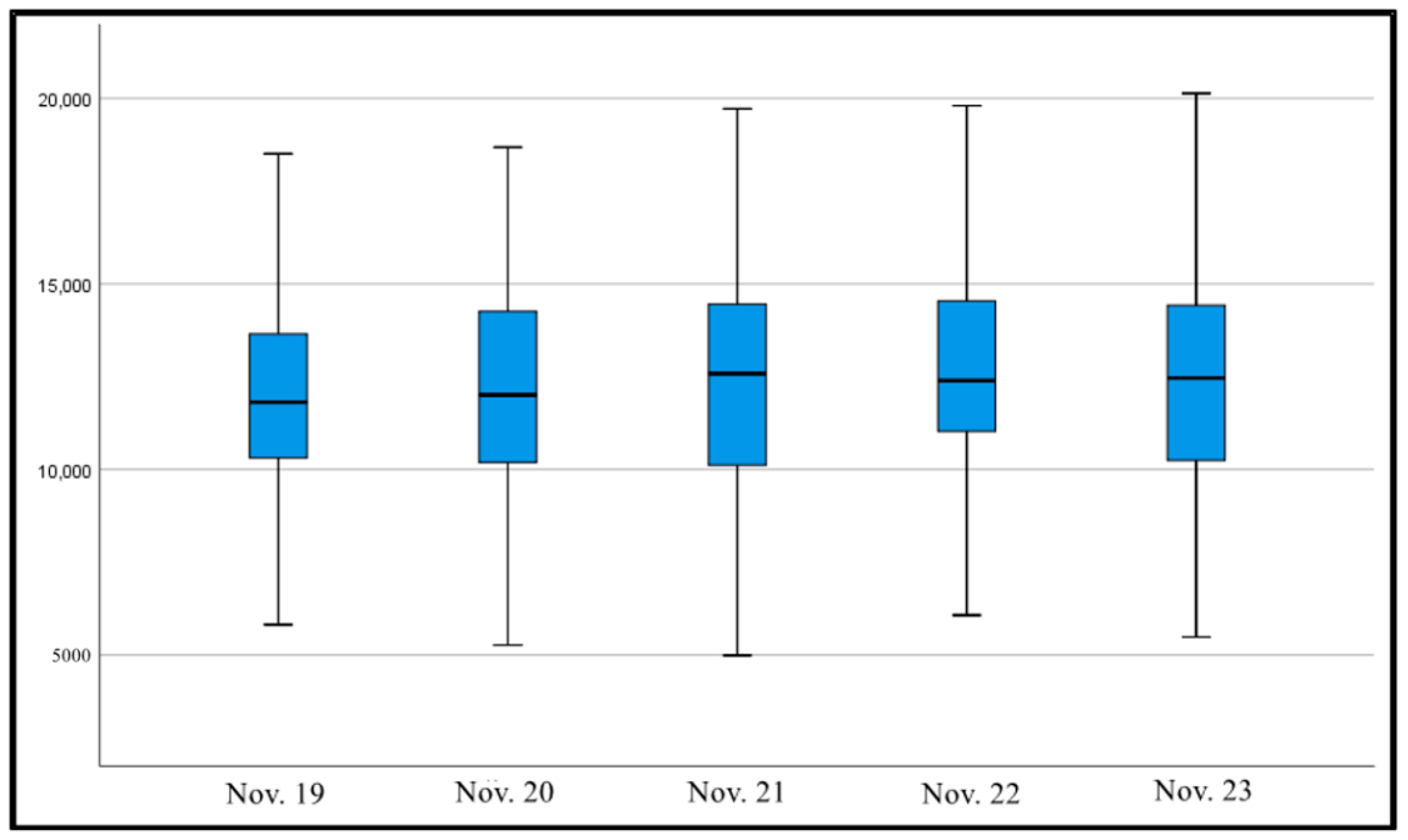
The total delay box line diagram for bus operation under different weather conditions is shown in Figure 5. The box line plot shows that the median, upper quartile, and lower quartile delays do not differ significantly by date. This indicates that weather changes do not have a significant impact on the operation of the 101 bus vehicles.

Figure 5. Box plot of delay statistics for different weather conditions.

Similarly, the average values of delays of different license plates at the same time period within 5 days are counted, as shown in Figure 6. The average values of delays exhibited by different license plates at the same time period have a uniform pattern, with a significant increase in delay values during peak periods. It shows that driver behavior also has little impact on the health of public transport operations, which is consistent with the conclusions of the correlation analysis.

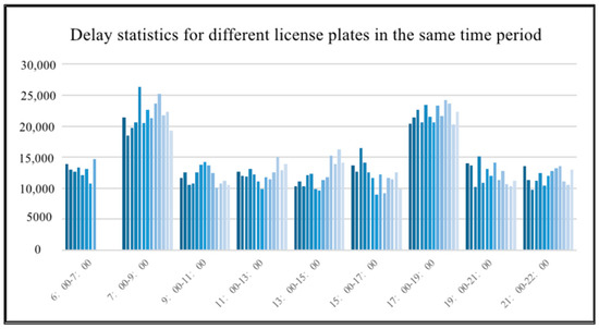
Figure 6. Delay statistics for different license plates at the same time.

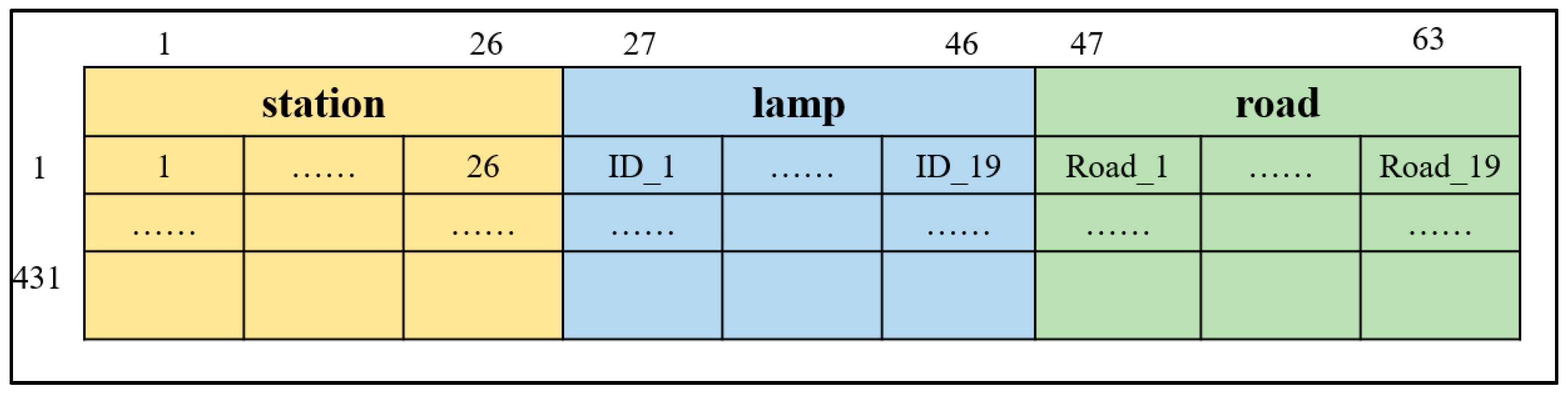
Therefore, this paper focuses on constructing feature sets with delay factors and constructing a random forest algorithm to study the key factors affecting the health of bus operation. Merging the three types of features, the final features of each bus trip are represented by a 63-dimensional vector, as shown in Figure 7.

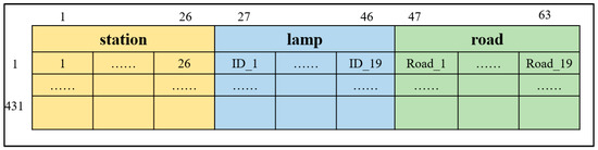
Figure 7. Schematic diagram of the feature set of influencing factors.

Based on this, a decision tree classification algorithm is used to judge the health classification for each trip as the data label, and the above 63 × 431 dimensional matrix is used as the feature set to construct the data set, and a random forest algorithm is used to construct a model to explore the degree of influence of different influencing factors on Foshan Bus Route 101.

3. Causes of Health in Public Transport Operations

3.1. Random Forest Algorithm Based on Bagging

(1) Principle of algorithm

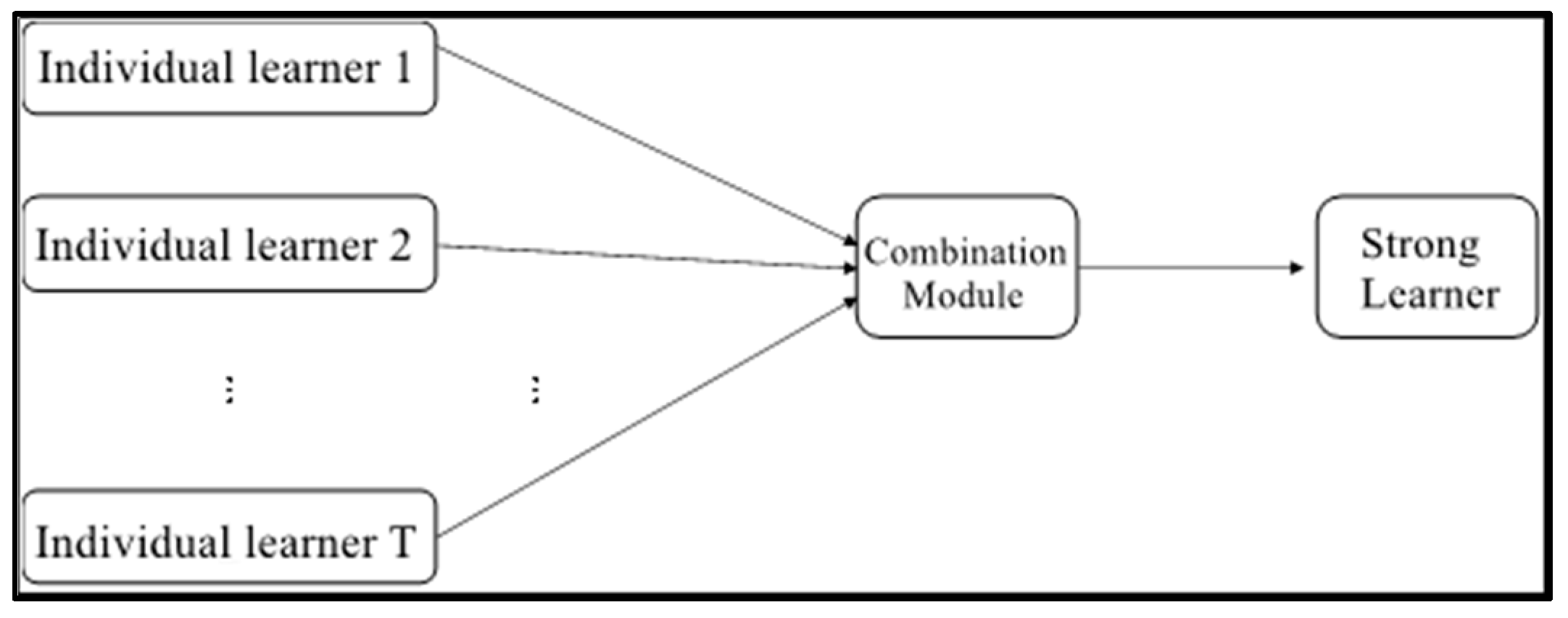
Among machine learning methods, in addition to single learning algorithms such as decision trees and Knn, there is also the very popular Ensemble learning machine learning algorithm. Figure 8 shows the schematic diagram of integration learning. Integrated learning refers to training several individual learners on the training set, and then combining them with some strategy to form a strong learner. This method of combining several individual learners usually provides better generalization performance than a single learner.

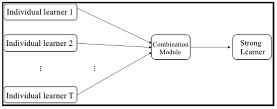
Figure 8. Schematic diagram of integrated learning.

The Random Forest (RF) algorithm is an integrated learning algorithm based on the Bagging algorithm, which represents a parallel integrated learning algorithm that generates several individual learners without dependencies in parallel. Bagging is based on the Bootstrap sampling method, where T sampling sets are collected from a training set D containing Bagging is based on bootstrap sampling, which collects T samples from a training set D containing m samples to train individual learners, each sample set is as large as the original training set. The bootstrap sampling method means that each time a random sample is taken from the training set D and put into the sampling set, and then the sample is put back into the training set D, so that the sample still has a chance to be selected in the next sampling. By randomly sampling the training set D m times, a sampling set containing m samples can be obtained. Following the above steps, T sample sets containing m samples can be sampled, and then T individual learners can be trained. Finally, the T individual learners are combined to obtain a strong learner. When combining the outputs of the individual learners, the simple averaging method is used for the prediction of the regression problem, i.e., the average of the prediction results of all individual learners is used as the prediction result of the integrated learner. For the classification problem, the simple voting method is used, i.e., the one with the highest number of predicted samples x belonging to the category of T individual learners is used as the final classification category.

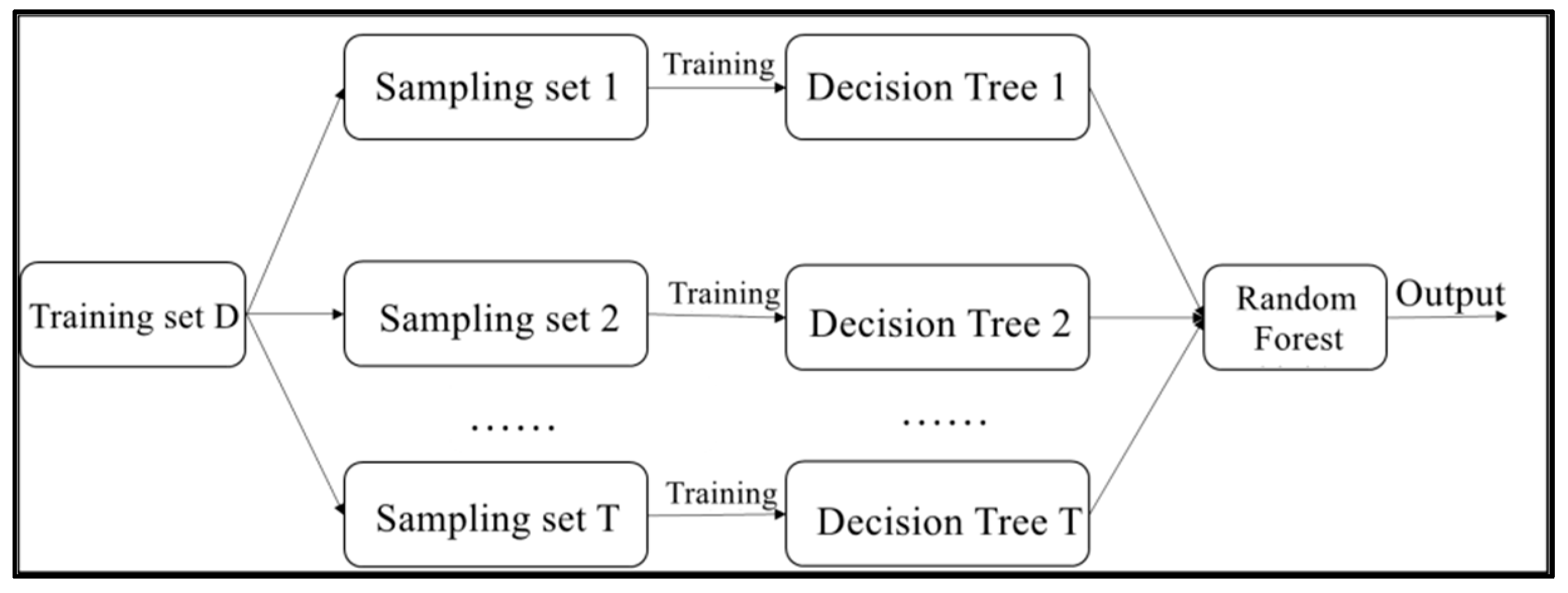
Random Forest is an extended version of Bagging. Figure 9 shows a schematic diagram of the learning process of Random Forest. Random Forest is an integrated machine learning algorithm that uses CART decision trees as individual learners. First, T sample sets are sampled from a training set D containing m samples by a self-service sampling method. Then, each sampled set is learned using a decision tree. Random forest is called an extended version of Bagging, because it builds on the Bagging integration by introducing random feature selection when training decision trees. The traditional decision tree algorithm selects an optimal feature from all the features of the current node when selecting the nodes of the tree for dividing the features. In contrast, decision trees in random forests are constructed by first selecting a random subset of features from all the features of the current node and then selecting an optimal feature from the subset of features. This can further enhance the generalization performance of the integrated learner. Finally, the prediction results for the samples are cast using the simple voting method.

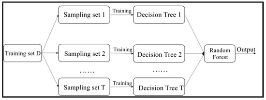
Figure 9. Schematic diagram of the random forest learning process.

The algorithm flow is shown in Table 6.

Table 6. Random forest algorithm flow.

Random Forest Algorithm
1: Input: Dataset $\mathrm{D}=\left\{\left({\mathrm{x}}_1,{\mathrm{y}}_1\right),\cdots ,\left({\mathrm{x}}_{\mathrm{m}},{\mathrm{y}}_{\mathrm{m}}\right)\right\}$, Feature set $\mathrm{T}=\left\{{\mathrm{t}}_1,\cdots ,{\mathrm{t}}_{\mathrm{d}}\right\}$ k: k-base learners (Decision Tree Learners) 2: Take 70% of the data as training set ${\mathrm{D}}_{\mathrm{tr}}$ and 30% of the data as test set ${\mathrm{D}}_{\mathrm{te}}$ randomly
2: for i = i to k do 3: N samples are taken from data set D as the training set ${\mathrm{D}}^{*}$ for the i decision tree randomly and with put-back 4: Specify the constant $\mathrm{m}<\mathrm{M}$ and randomly select a subset of m features from M features to form the feature set ${\mathrm{T}}^{*}$ 5: Build a decision tree model, TreeGenerate $({\mathrm{D}}^{*},{\mathrm{T}}^{*}$), where each tree is grown to the maximum extent possible 6:  end for 7: Generate k decision tree models
8: All k models make classification predictions for test set ${\mathrm{D}}_{\mathrm{te}}$ and return the most classified classification labels

(2) Evaluation of the importance of influencing factors

The random forest model can output the magnitude of the influence of each influence factor on the health rating of public transportation operations. The variable importance score is a measure of the influence of the corresponding variable using the reduction in model accuracy. Using noise data randomly added to each characteristic variable, the value of the change in accuracy of the random forest model is calculated, and the importance of the variable is evaluated according to the magnitude of the change in accuracy. If the accuracy of the model increases after reducing the noise of a certain independent variable, the importance of that variable is higher. The formula for calculating the importance of the influencing factor characteristic $t$ is:

$$I(t)=E_O(g)-E_O^{(n)}(g)$$

(6)

In Formula (6), $E_O(g)$ is the out-of-bag error of the random forest model. $E_O^{(n)}(g)$ indicates the new out-of-bag error of the random forest when the value of feature $t$ is perturbed by noise. The larger the value of $I\left(t\right)$, the greater the effect of the disturbing feature $\mathrm{t}$ on the out-of-bag error of the random forest, indicating its greater impact on the health of the transit operation.

3.2. Random Forest Model Optimization and Evaluation

(1) Category imbalance problem

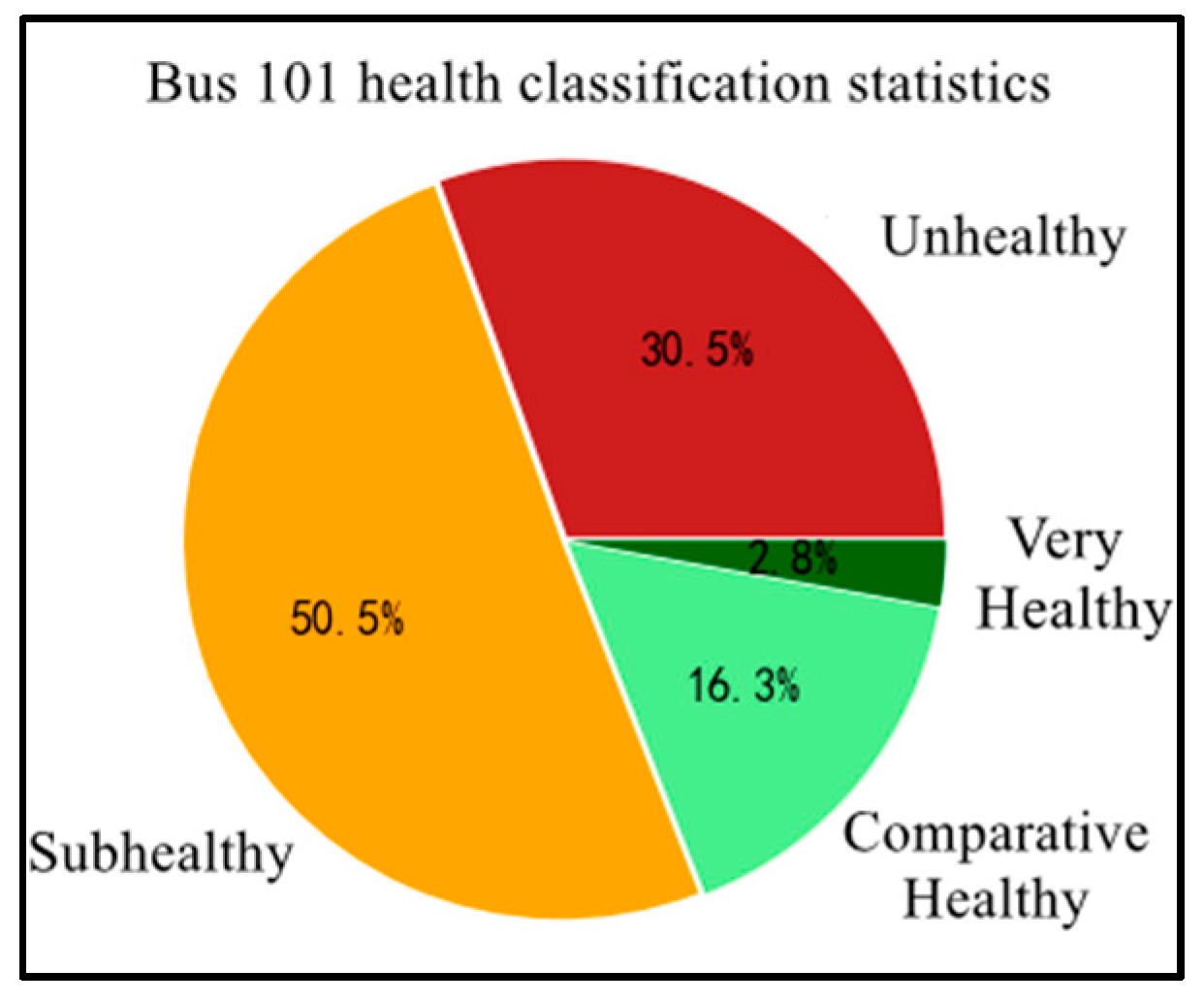
The decision tree algorithm was used to judge the bus operation health class of Foshan Bus 101 for a total of 431 trips from 21 November to 25 November 2016. The statistics are shown in Figure 10.

Figure 10. Statistical chart of 101 road health level judgment.

It can be seen that the samples are very unevenly distributed under the four health class categories, and the category imbalance can produce a significant interference in the learning process of the model, thus affecting the performance of the model. In a multi-categorization task, if the number of samples in different categories differs significantly, it is difficult for the learner to learn effective information from the category with a small number of samples, which results in the category with a small number of samples being incorrectly predicted as the category with a larger number of samples.

An improved SMOTE oversampling algorithm proposed by Chawla [32] is used to solve this problem. The algorithmic flow of the SMOTE algorithm for sampling the samples is as follows.

(1) For a sample $x_i$ in a few categories, calculate its Euclidean distance from the surrounding samples and find the $k$ nearest neighbors at the distance.

(2) Select a sample $x_n$ from the $k$ nearest neighbors randomly.

(3) Synthesize a new sample according to $x_i$ and $x_n$ according to the following formula.

$$x_{new}=x_i+random(0,1)\ast |x_i-x_n|$$

(7)

In Formula (7), $random\left(0,1\right)$ denotes the generation of random numbers between 0 and 1. Instead of sampling the original samples by simply copying them randomly, the SMOTE algorithm generates new samples based on the original data by a determined algorithm, thus effectively alleviating the overfitting problem. In this paper, the SMOTE algorithm is used to achieve a ratio of 1:1:1:1 for the four types of samples.

(2) Optimization of algorithm parameters

Random forest algorithm differs from decision tree algorithm in that the main parameter is the n_estimators of the decision tree, and other algorithms are the same as decision tree. The common order of parameter optimization is: n_estimators, max_depth, max_features, min_samples_leaf, min_impurity_decrease.

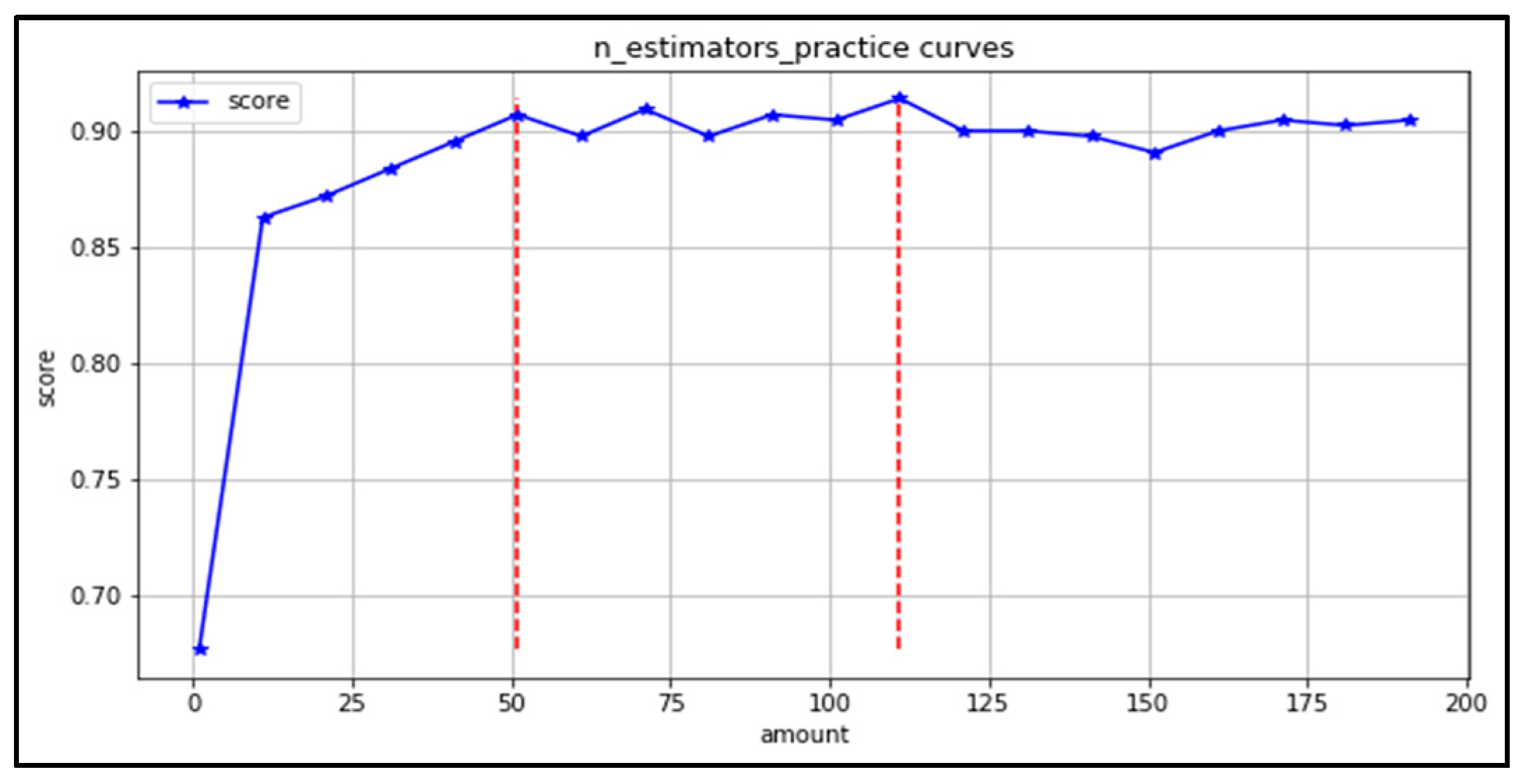
(1) n_estimators: refers to the number of tree models in the random forest, this parameter determines the size of the forest. If the n_estimators value is too small, it is easy to under-fit. However, if the value of n_estimators is too large, the forest is too large, which will increase the training time of the model. Draw the learning curve of n_estimators in the range (0–200). It can be seen from Figure 11 that the results are better in the range (50,120), and the model accuracy does not change much beyond 120. Therefore, the grid search range is (50,120).

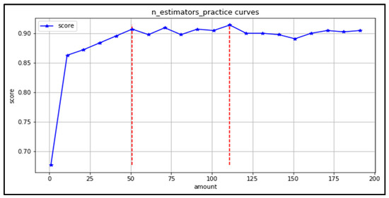
Figure 11. Decision Tree Trees Learning Curve.

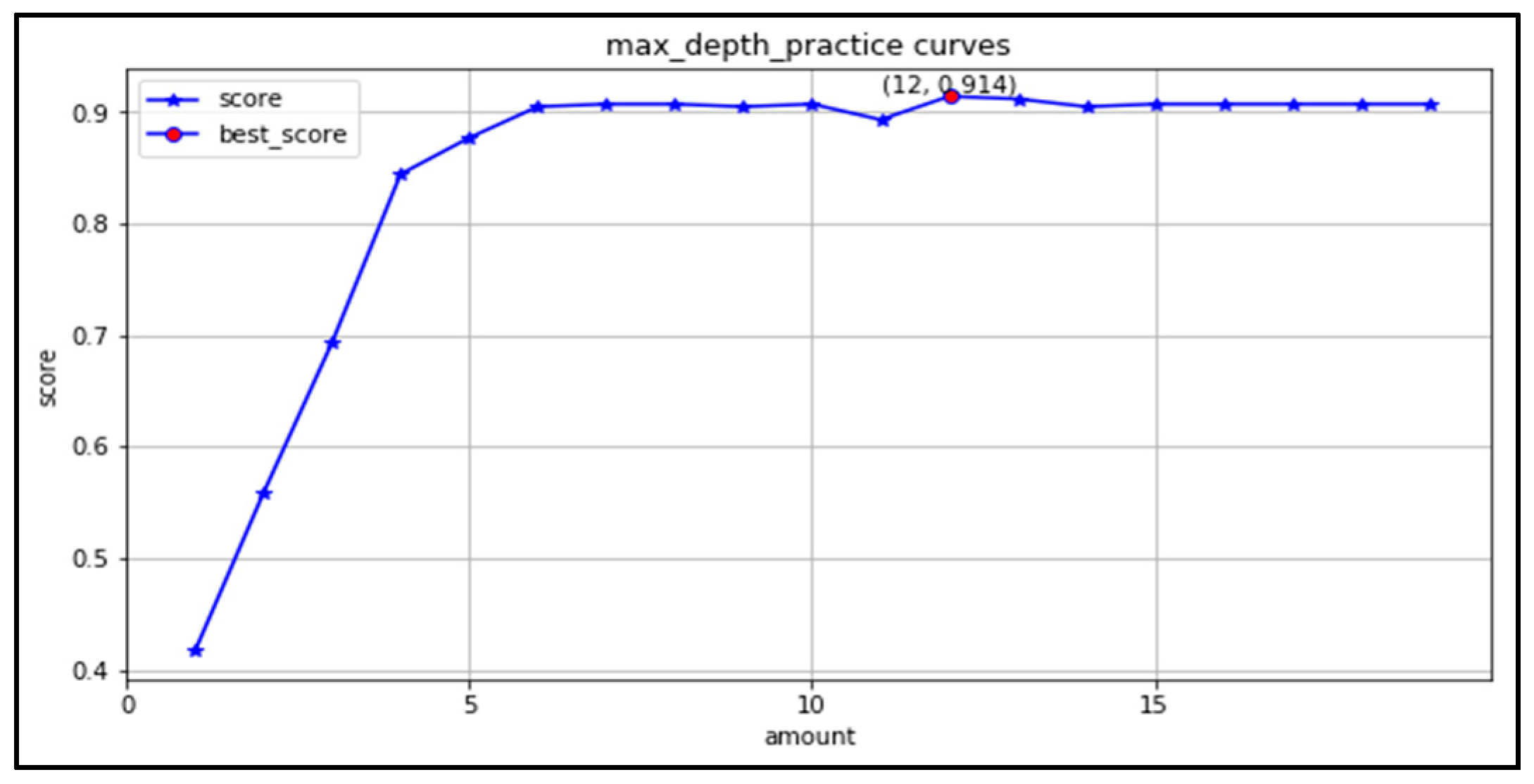
(2) max_depth: the learning curve is plotted in the range (1,20), as shown in Figure 12. The optimal range of maximum depth is (6,20). The highest accuracy is 0.914 when taking 12.

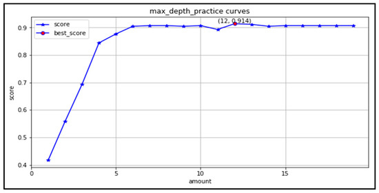
Figure 12. Maximum depth learning curve.

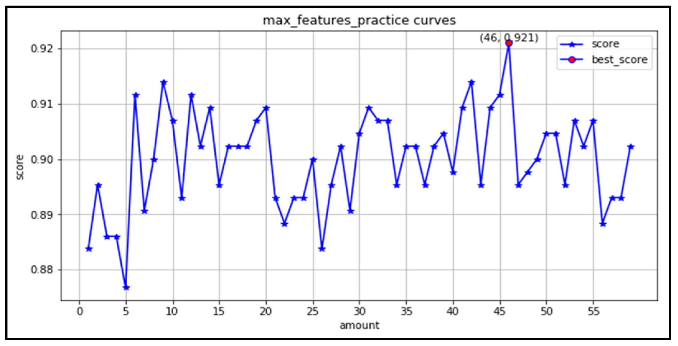
(3) max_features: There are 63 features in this study, thus the learning curve is plotted for the maximum number of features in the range of (1,63). As seen in Figure 13, the best result is achieved with an accuracy of 0.921 when the maximum features are taken as 46. The maximum number of features is searched in the range (6,55) for grid search.

Figure 13. Maximum number of features learning curve.

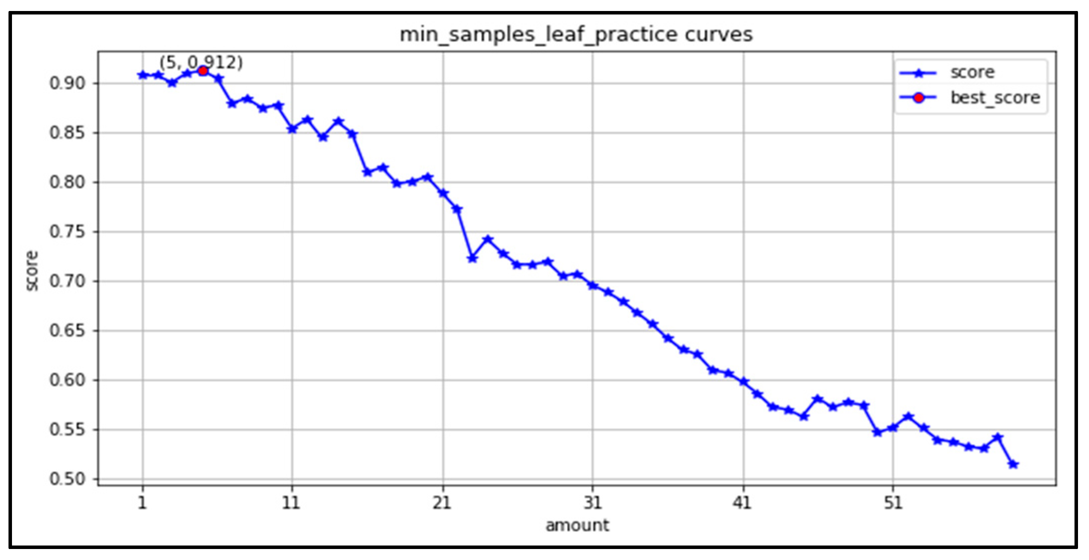
(4) min_samples_leaf: the learning curve is plotted in the range (1,60). As seen in Figure 14, the minimum number of leaves works best in the range (1,5). As the parameter increases, the accuracy decreases.

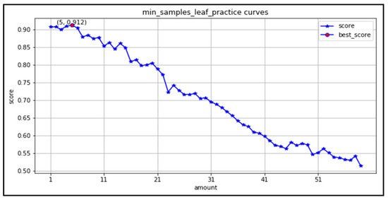
Figure 14. Learning curve of minimum number of leaves.

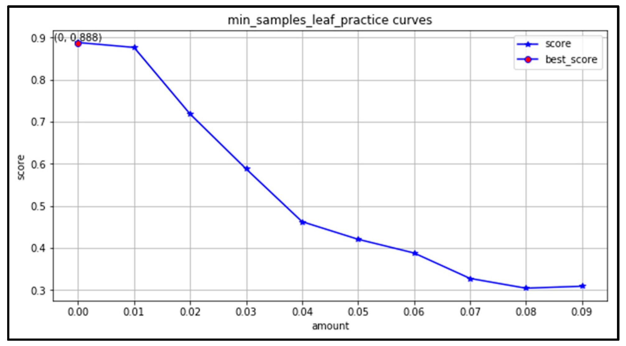
(5) min_impurity_decrease: the learning curve is plotted in the range of (0,1) with an interval of 0.01. From Figure 15, it can be seen that the accuracy is highest when the minimum information gain is 0. Additionally, as the information gain increases, the accuracy rate decreases, indicating that the minimum information gain parameter adjustment will have a negative impact on the model. Therefore, the optimal parameter of the minimum information gain is 0 by default in the grid search.

Figure 15. Minimum information gain learning curve.

According to the above optimal parameter ranges, n_estimators range is (50,120), max_depth range (6,20), max_features range (1,63), and min_samples_leaf range (0,5). The optimal parameters derived from the grid search method are shown in Table 7. The accuracy rate reaches 0.926.

Table 7. Optimal parameter values.

Parameters	Value
n_estimators	111
max_depth	15
max_features	52
min_samples_leaf	1
min_impurity_decrease	0

(3) Evaluation of algorithm effects

The decision tree algorithm and the Knn algorithm were used to model the classification of the constructed dataset separately and the results were compared. From Table 8, it can be seen that the random forest algorithm has the best results.

Table 8. Algorithm evaluation results.

Algorithms	Accuracy
Knn	0.721
Decision Trees	0.842
Random Forest	0.926

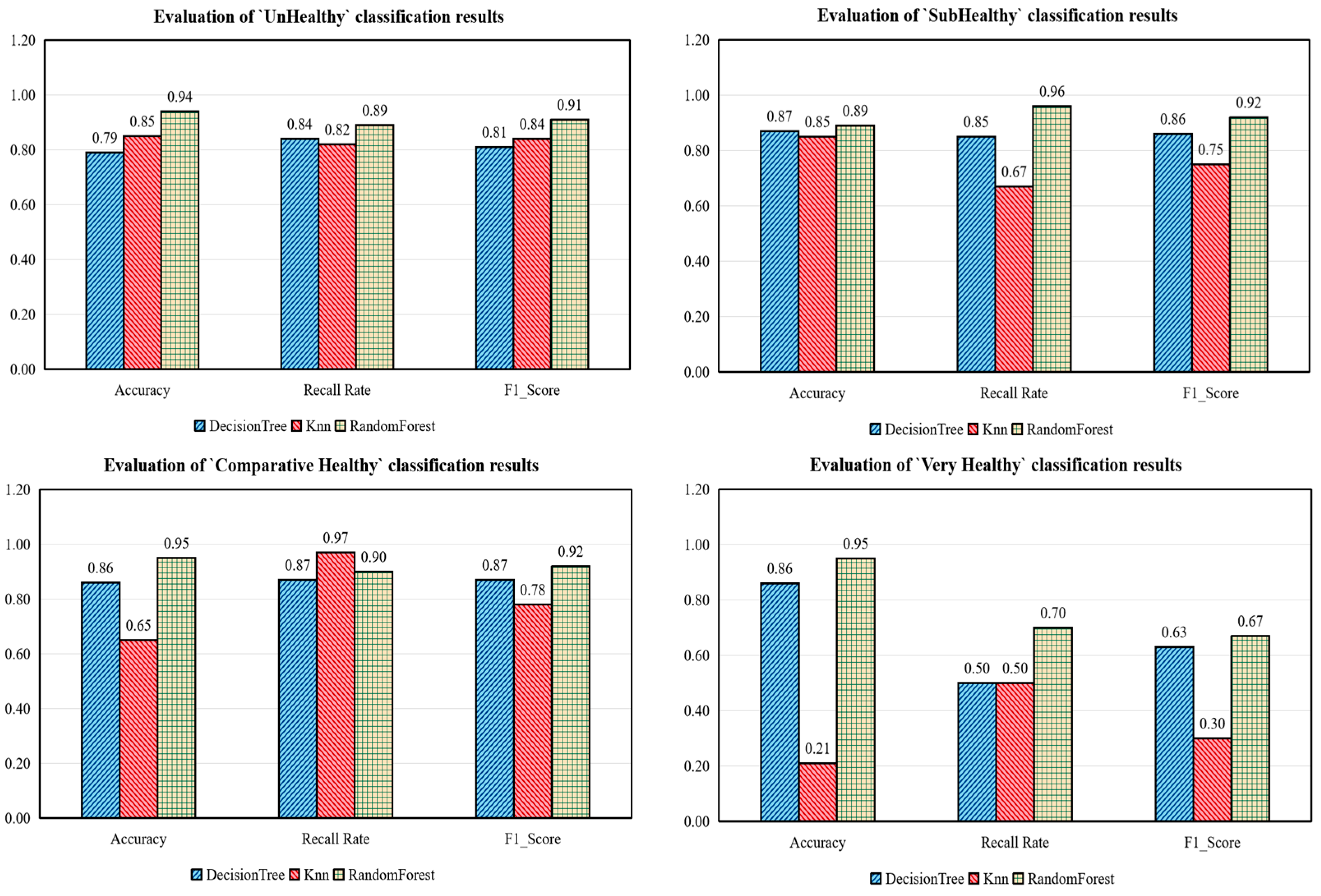
The evaluation metrics of each classification label are shown in Figure 16. Random Forest outperforms the other two algorithms in all health classes. In particular, in the “very healthy” classification level, the random forest algorithm performs much better than the other two algorithms due to the small number of very healthy samples.

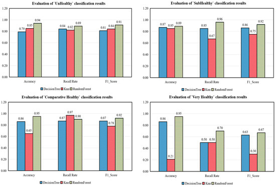
Figure 16. Algorithm evaluation.

3.3. Analysis of the Causes of Public Transportation Operational Health

The random forest model was used to quantify the importance of different influencing factors features and analyze the key factors affecting the operational health of Foshan Bus Route 101 in detail. Table 9 shows the statistical table of the importance of different characteristics of the influencing factors; road_x represents the road section number, ID_x represents the intersection number, and x_station represents the station number.

Table 9. Statistical table for ranking the importance of influencing factors.

Feature	Importance	Rank	Feature	Importance	Rank	Feature	Importance	Rank
road_10	0.1997	1	ID_6	0.0129	22	ID_4	0.0059	43
road_4	0.0945	2	road_2	0.0123	23	6station	0.0056	44
ID_10	0.0586	3	road_1	0.012	24	19station	0.0055	45
road_3	0.0361	4	3station	0.0119	25	road_19	0.0053	46
road_16	0.0342	5	ID_11	0.0114	26	ID_3	0.0052	47
road_5	0.0256	6	ID_13	0.0109	27	ID_15	0.0052	48
road_9	0.0252	7	ID_1	0.0102	28	ID_12	0.0052	49
road_12	0.0247	8	ID_14	0.0102	29	9station	0.0052	50
road_11	0.0239	9	21station	0.0101	30	ID_16	0.005	51
road_7	0.0223	10	4station	0.0098	31	2station	0.005	52
ID_18	0.0185	11	ID_9	0.0095	32	ID_7	0.0047	53
ID_5	0.0174	12	14station	0.0088	33	5station	0.0047	54
16station	0.0174	13	25station	0.0081	34	road_15	0.0045	55
road_8	0.0163	14	road_17	0.008	35	ID_17	0.0045	56
ID_2	0.0152	15	road_13	0.0078	36	15station	0.0038	57
1station	0.0151	16	22station	0.0069	37	7station	0.0035	58
18station	0.0144	17	ID_19	0.0066	38	8station	0.0034	59
13station	0.0143	18	12station	0.0066	39	23station	0.0032	60
road_6	0.0137	19	17station	0.0064	40	11station	0.003	61
road_14	0.0137	20	20station	0.0063	41	24station	0.0025	62
road_18	0.0131	21	ID_8	0.006	42	10station	0.0025	63

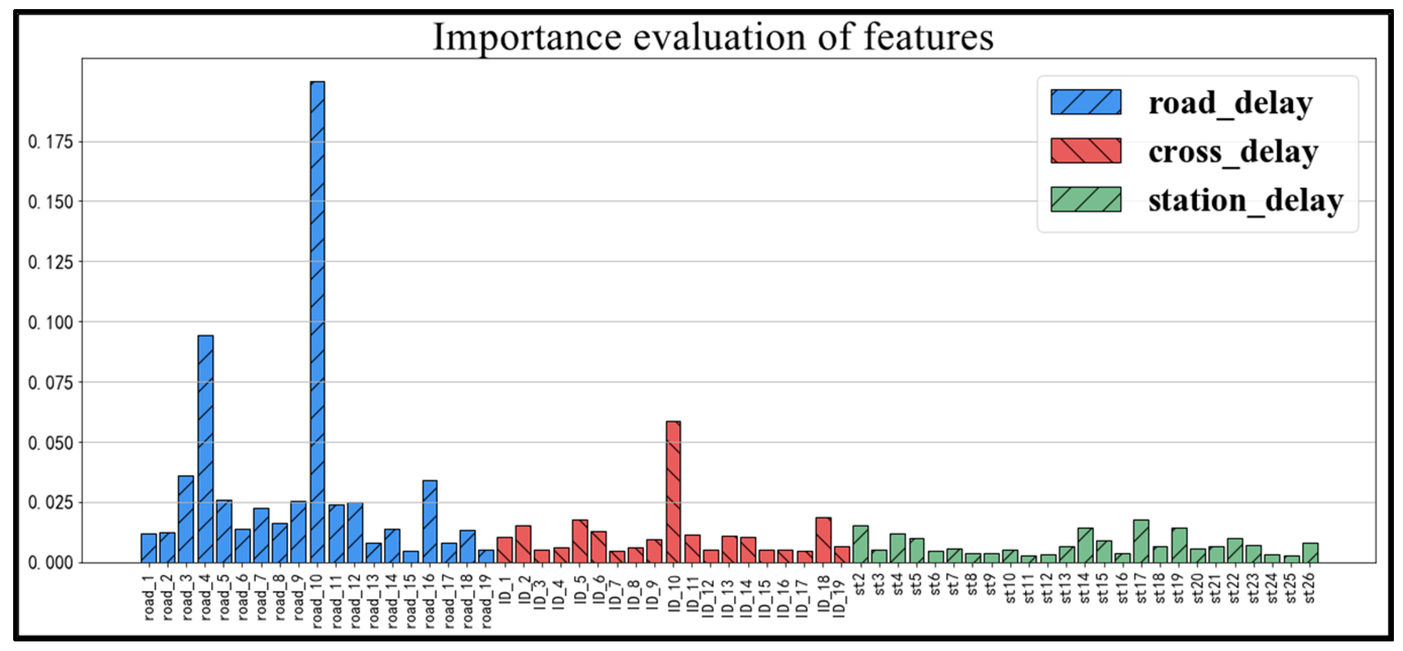
The importance scores were categorized according to road delays, cross delays, and station delays, as shown in Figure 17.

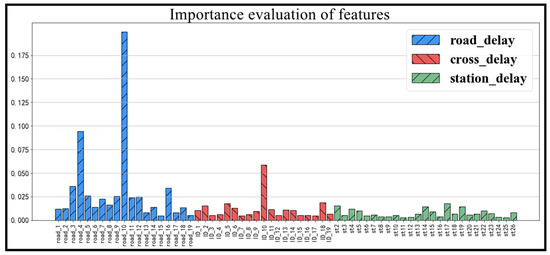
Figure 17. Statistical chart of feature importance classification.

The categorical statistical chart shows that road delay is the main factor affecting the health of bus operations. Inter-section congestion accounts for the largest share. Cross delay also has an impact on transit operational health, while station delay has the least impact on transit operational health status. The top five key influencing factors are road Section 10, road Section 4 and inter Section 10, road Section 3 and road Section 16, with the importance of influencing factors of 0.1997, 0.0945, 0.0586, 0.0361, and 0.0342, respectively.

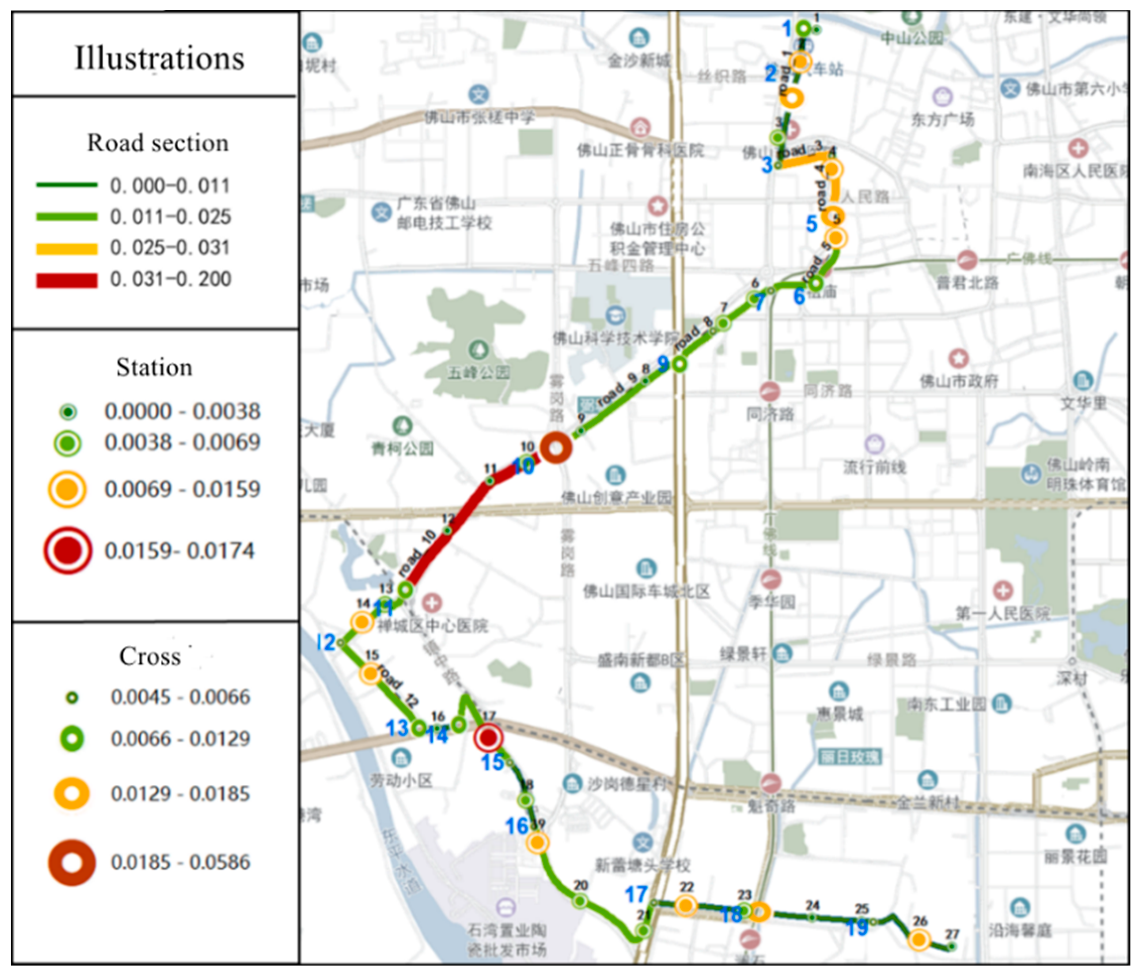
Visual analysis was performed in ArcGIS based on the statistical table, as shown in Figure 18.

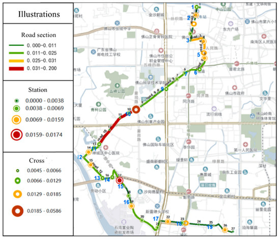
Figure 18. Visualization of the ranking of influence factors.

From the figure, it can be seen that the biggest impact on the health of bus operation is Section 10, i.e., the section from site 10 to site 13, which is the bottleneck of bus operation. According to the analysis of the visualization results, when a road section is more affected by road delay, it is also more affected by cross delay. It means that cross delays and road delays are mutually influential. When traffic congestion occurs on a section, it affects the intersection queue length and leads to increased cross delays on the next section. When the cross delay or station delay is large, it means that this intersection is congested, which will lead to the next road delay larger. Station delays are mainly related to passenger flow, thus there is less correlation with cross delays and road delays. However, when the road delay has a large impact, the station delay will appear to have little impact. It is due to bus drivers compressing stop times to improve punctuality when there are large road delays or cross delays. In this case, the impact of station delay is significantly reduced.

4. Conclusions

This paper analyzed the influencing factors and calculations that affect the operational health of public transport. Taking Foshan bus route 101 as an example, the delays at each road section, intersection and station were calculated separately. Afterwards, a random forest algorithm was used to construct a causal analysis model for health diagnosis, and the importance ranking and scoring of different influencing factors were output. Finally, visualization of the different categories of influencing factors was carried out to make the invisible information visible in the data. The simulation results prove that the method can quickly, accurately, and intuitively find the operational bottlenecks and Intrinsic causes of bus routes with good results.

The advantages of this method over traditional methods include two aspects:

(1)

The study quantitatively determines the extent to which different factors affect the health of bus operations. It changes the limitations of previous studies that only find the symptoms, but not the causes of the disease.

(2)

The model is based on basic information about public transport operations, which is easily accessible. The method is uncomplicated to implement, and the results are highly accurate and usable. It can be universally applied to conventional public transport scenarios.

The content of this paper focuses on the diagnosis and cause analysis of bus operation conditions based on historical data. Subsequent research can predict the operating conditions of public transport, study future trends in health conditions, and improve practical guidance.

References

- Qian, L.H. The fundamental way to solve the traffic problems of big cities is to vigorously develop public transportation. Beijing Plan. Constr. 1998, 6, 25–27. [Google Scholar]
- Shanghai Comprehensive Transportation Annual Report (2020). Traffic Transp. 2019, 34, 10–12.
- Wang, P.; Lin, J.J.; Barnum, D. Data envelopment analysis of bus service reliability using automatic vehicle location data. In Proceedings of the 86th Annual Meeting of Transportation Research Board, Washington, DC, USA, 9–13 January 2008. [Google Scholar]
- Liu, X.; Graham, D.J. Development of a Key Performance Indicator to Compare Regularity of Service between Urban Bus Operations. Transp. Res. Rec. J. Transp. Res. Board 2011, 2216, 33–41. [Google Scholar]
- Wei, Q.B.; Yang, J.F.; Chen, C.J. Study on the evaluation index system of public transport operation service in Guangzhou. Transp. Res. 2016, 2, 17–23. [Google Scholar]
- Wen, H.Y.; Wu, L.F.; Mei, J.J. Fuzzy Comprehensive Evaluation of Guangzhou-Foshan Intercity Bus Satisfaction Based on Improved AHP Method. J. Zhongshan Univ. (Nat. Sci. Ed.) 2018, 5, 64–71. [Google Scholar]
- Chen, Y.Y.; Cai, Y.W.; Hou, Y.M. Evaluation method of “health index” of bus routes in large cities. J. Changan Univ. Nat. Sci. Ed. 2015, 35, 1–6. [Google Scholar]
- Lin, Y.; Yang, X.; Zou, N. Real time bus arrival time prediction: Case study for Jinan. J. Transp. Eng. 2013, 11, 1133–1140. [Google Scholar] [CrossRef]
- Wang, C. Research on the evaluation system of road traffic health status in old urban areas. Urban Roads Flood Control 2016, 12, 143–147. [Google Scholar]
- Zheng, C.J.; Zhang, Y.H.; Feng, X.J. Improved iterative prediction for multiple stop arrival time using a support vector machine. Transport 2012, 2, 158–164. [Google Scholar] [CrossRef]
- Ke, J.Y. Evaluation of transportation efficiency of bus routes based on improved DEA. In Proceedings of the 2018 Annual Conference on Urban Transportation Planning in China, Qingdao, China, 16–18 October 2018. [Google Scholar]
- Lu, H.P.; Yang, M.; Zhang, Y.B. Assessment of integrated development of comprehensive transportation hubs and suggestions for countermeasures. Compr. Transp. 2019, 4, 25–30. [Google Scholar]
- Shen, L.; Feng, T.; Mo, Y. Passenger perception-based service quality assessment of pick-up bus service. Highw. Transp. Technol. 2019, 8, 152–158. [Google Scholar]
- Zhang, L.; Panos, D.P. Signalized Intersection LOS that Accounts for User Perceptions. In Proceedings of the 83th Annual Meeting of the Transportation Research Board, National Research Council, Washington, DC, USA, 11–15 January 2004. [Google Scholar]
- Xin, G.Z. Research on Multi-Modal Bus Network Effectiveness Assessment Method. Master’s Thesis, Southeast University, Nanjing, China, 2015. [Google Scholar]
- Fan, L.J. Analysis of Bus Rapid Transit Operation Status and Service Level Classification. Master’s Thesis, Shandong University, Jinan, China, 2017. [Google Scholar]
- Ouyang, Y.; Nourbakhsh, S.M.; Cassidy, M.J. Continuum approximation approach to bus network design under spatially heterogeneous demand. Transp. Res. Part B Methodol. 2014, 68, 333–344. [Google Scholar] [CrossRef]
- Daniel, T.; Peng, Z.R. Timetable optimization for single bus line based on hybrid vehicle size model. J. Traffic Transp. Eng. 2015, 2, 179–186. [Google Scholar]
- Chou, C.H. Machine Learning; Tsinghua University Press: Beijing, China, 2016. [Google Scholar]
- Zhang, J.Q.; Shi, W.B.; Ji, X.J. Machine learning in healthcare and public health applications. China Public Health 2019, 10, 1449–1452. [Google Scholar]
- Zhang, R.; Wang, Y.B. Research on machine learning and its algorithms and development. J. Commun. Univ. China Nat. Sci. Ed. 2016, 2, 10–18. [Google Scholar]
- Zhao, J.Y. Research and Application of Machine Learning Methods for Health Assessment. Master’s Thesis, University of Electronic Science and Technology, Chengdu, China, 2013. [Google Scholar]
- Fan, X.H. Research on Support Vector Machine Classification Algorithm. Master’s Thesis, Northwestern Polytechnical University, Xian, China, 2016. [Google Scholar]
- Zheng, Y.; Hu, X.P.; Yin, J. A multi-task support vector machine based approach to health data fusion. Syst. Eng. Theory Pract. 2019, 2, 418–428. [Google Scholar]
- Yu, M.J.; Wang, Y.L. Research on plain Bayesian classification algorithm. Bus. Intell. 2012, 8, 226–227. [Google Scholar]
- Zhang, G.W.; Wang, L.; Wang, X.Y. Research on sand information extraction method based on CART decision tree. Arid Zone Geogr. 2019, 5, 1133–1140. [Google Scholar]
- Champahom, T. Evaluating user’s satisfaction of bus service in Mauritius: Decision tree approach. Lowl. Technol. Int. 2019, 4, 478–489. [Google Scholar]
- Zhu, S.Z. A study based on the implementation of k-nearest neighbor algorithm. Comput. Digit. Eng. 2015, 10, 1771–1774. [Google Scholar]
- Xiao, J. Research on the Classification Method of Imbalanced Data Based on Random Forest. Master’s Thesis, Harbin Institute of Technology, Harbin, China, 2013. [Google Scholar]
- Li, Q. Characterizing the importance of criminal factors affecting bus ridership using random forest ensemble algorithm. Transp. Res. Rec. 2019, 4, 864–876. [Google Scholar] [CrossRef]
- Zhou, Y. Evaluation Method of Bus Operation Based on Vehicle Positioning Data. Master’s Thesis, Southeast University, Nanjing, China, 2015. [Google Scholar]
- Chawla, N.V.; Bowyer, K.W.; Hall, L.O. SMOTE: Synthetic Minority Over-sampling Technique. J. Artif. Intell. Res. 2002, 1, 321–357. [Google Scholar] [CrossRef]
Publisher’s Note: MDPI stays neutral with regard to jurisdictional claims in published maps and institutional affiliations. |
© 2021 by the authors. Licensee MDPI, Basel, Switzerland. This article is an open access article distributed under the terms and conditions of the Creative Commons Attribution (CC BY) license (https://creativecommons.org/licenses/by/4.0/).