Parallel Hybrid Electric Vehicle Modelling and Model Predictive Control

Abstract

This paper presents the modelling and calculations for a hybrid electric vehicle (HEV) in parallel configuration, including a main electrical driving motor (EM), an internal combustion engine (ICE), and a starter/generator motor. The modelling equations of the HEV include vehicle acceleration and jerk, so that simulations can investigate the vehicle drivability and comfortability with different control parameters. A model predictive control (MPC) scheme with softened constraints for this HEV is developed. The new MPC with softened constraints shows its superiority over the MPC with hard constraints as it provides a faster setpoint tracking and smoother clutch engagement. The conversion of some hard constraints into softened constraints can improve the MPC stability and robustness. The MPC with softened constraints can maintain the system stability, while the MPC with hard constraints becomes unstable if some input constraints lead to the violation of output constraints.

1. Introduction

Controllers for HEVs powertrains and speeds can be included model-free or model-based. Model-free controllers are mostly used with heuristic, fuzzy, neuro, AI, or human virtual and augmented reality. The use of model-free methods will be presented in the next part of this study. Model-based controllers can be used with a conventional adaptive PID, H₂, H_∞, or sliding mode. However, all conventional control methods cannot include the real-time dynamic constraints of the vehicle physical limits, the surrounding obstacles, and the environment (road and weather) conditions. Therefore, a MPC with horizon state and open loop control prediction subject to dynamic constraints are mainly used to control as real-time the HEV speeds and torques. Due to the limit size of this paper, we have reviewed some of the most recent research of MPC applications for HEVs. In this paper, vehicle dynamic formulas and calculations are referred to the reference [1].

A recent modelling and control of the dual clutch transmission for HEVs are presented in [2], in which a new controller was designed for synchronizing the dual clutch transmission (DCT) with higher performances and lower fuel consumption. Another MPC for an autonomous driving vehicle is developed in [3], in which the MPC was used to drive the HEV to exactly track the given feasible trajectories. Moreover, a controller for a hybrid dual clutch transmission powertrain for a HEV is introduced in [4], in which the ICE and EM were driven by a DCT powertrain. A MPC for a HEV with linear parameters and a varying model is presented in [5], in which the MPC controller was designed to improve the fuel economy of the power-split HEV.

A MPC for a HEV is necessary not only to control the torque and speed, but also to control the gas emission and improve the fuel economy. The authors of [6] developed a MPC with a multi-objective function for HEVs for fuel economy and exhaust emission and collision detection as well as to optimize the vehicle speed and engine torque. A new MPC design for HEVs with adaptive cruise of autonomous electric vehicles was presented in [7]. A hybrid MPC to optimize the HEV mode selection was introduced in [8], in which the vehicle thermal management was controlled by this MPC subject to decision-making algorithms. Fuel economy and lower emission were also controlled by a MPC with outer approximation and semi-convex cut generation, as presented in [9].

Due to the recent world commitment to limit the increase in global warming and stop using fossil fuels, plug-in and the pure electric vehicles are expanding. MPC algorithms are also being developed to control the plug-in hybrid vehicle (PHEV), as shown in [10]. In this study, a non-linear MPC is designed to control the torque-split and to optimize fuel management. The authors of [11] also present a data-based scenario MPC framework to optimize power consumption.

Non-linear model predictive control (NMPC) has been widely used due to the rapid increase in computer capacity and speeds. Computers now can calculate a real-time solution from complex non-linear functions. Therefore, the authors of [12] provide a MPC for the non-linear energy management of the power split HEV. Energy efficiency management for HEVs is now also extended in communication among vehicles, as shown in [13], in which a MPC framework is proposed to generate the optimal torque and velocity by connecting the information from vehicle to vehicle.

The authors of [14] reviewed the latest model-based controllers in the market to assess the improvement of energy management for HEVs, and, in this study, the MPC was used to calculate optimal energy, torque, and speed. Since a MPC is a model-based algorithm, difficulties will arise when there are existing mismatches between the model and the plant or the plant uncertainties. These mismatches and uncertainties may lead to the instability of the controller. Robust model predictive control (RMPC) algorithms are, therefore, developed to deal to these uncertainties. The authors of [15] present a new method using matrix inequalities based on RMPC for HEVs considering the external disturbances, the time varying delays, and the model uncertainties. The authors of [16] introduce a real-time NMPC for the energy management of HEVs using sequential quadratic programing.

The use of a MPC for pure electric vehicles is also mentioned in [17] regarding full battery consumption and road slope condition. The authors of [18] presented a decentralized MPC of plug-in electric vehicles charged based on the alternative direction method of multipliers. A real-time control for HEVs, longitudinal tracking, jaw movement, dual-mode power split, and minimizing energy were presented by the authors of [19,20,21,22,23,24,25,26,27,28]. However, none of the recent MPC methods mentioned is concerned with the MPC with softened constraints. The MPC is always subject to many strict constraints on states, outputs, and inputs; therefore, the MPC may not find a feasible solution and it may become unstable. Since the MPC is a real-time optimizer, any failure solution cannot be tolerated. We propose to convert some physical strict constraints into softened constraints, while adding some large penalty values into the MPC objective function. In this way, we can increase the stability and the robustness of the system dealing with uncertainties and some initial conditions, which may lead the input to violate output constraints.

The layout of this paper is as following: Section 2 presents the modelling of the parallel HEV; Section 3 introduces the design of the MPC; Section 4 develops the MPC algorithms with softened constraints; Section 5 illustrates the simulations of the MPC for the HEV; and Section 6 is the conclusion.

2. Modelling of the Parallel HEV

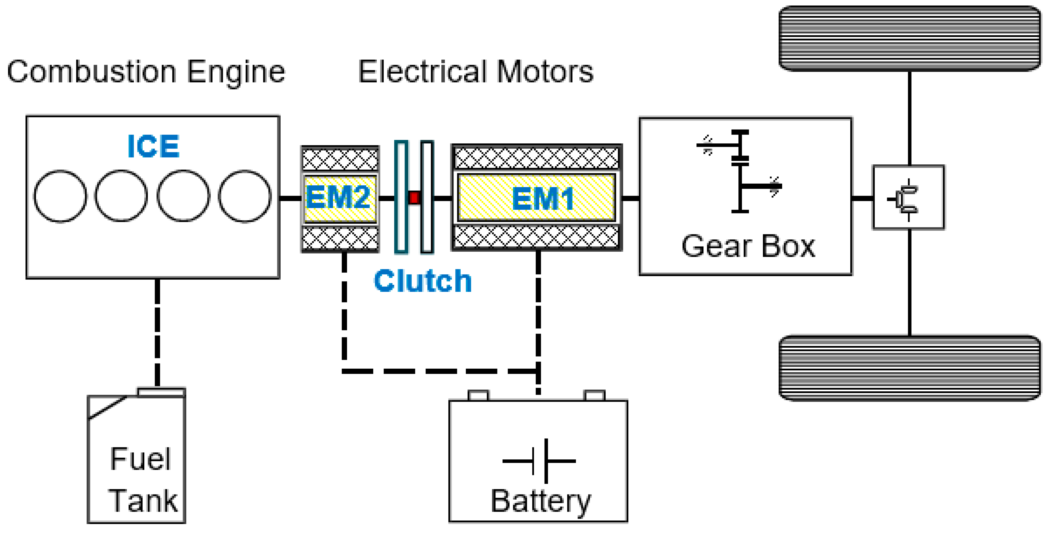
In parallel hybrid electric vehicles, both combustion engine and main electric motor are installed in parallel and work in independent configurations. The vehicle can run and switch in four driving modes: pure main electric motor (EV1) at a low speed and/or low load; pure combustion engine (EV2) at a high speed and/or high load; both main electric motor and combustion engine (EV3) at a very high and/or very high load; and a combination of the main electric motor, generator motor, and combustion engine (EV4) at extreme high speed and/or load. In 2021, Hyundai introduced a new version of Sonata Hybrid, the middle size family passenger HEV that combines updated technologies for a typical parallel electric vehicle, as shown in Figure 1.

This parallel HEV consists of one internal combustion engine (ICE) with four cylinders with multiple point injection, a volume of 2.4 litters, a maximum power of 156 kW at 6000 rpm, and a peak torque of 265 Nm; one electric motor starter (EM2) with a maximum power of 8 kW and a maximum torque of 43 Nm; the main electric motor (EM1) with a maximum power of 35 kW and a maximum torque of 205 Nm; the battery HEV Li-ion with a capacity of 6.1 Ah; a transmission gearbox with fully automated 6 speeds; and a friction clutch engagement. The vehicle curb weight is 1569 kg. This Sonata Hybrid vehicle is used to simulate our system modelling and test the new MPC scheme with softened constraints.

The schematic architecture of the 2021 Hyundai Sonata Hybrid in Figure 1 can be modelled with a simple drivetrain and is shown in Figure 2. The first part of this mechanical structure consists of an internal combustion engine (ICE) and the electric starter/generator motor (EM2) can be grouped into one inertia $J_1$, including the left clutch disk, the sharp 1, EM2, and ICE. $J_1$ is modelled as one rigid inertia. $M_{ICE}$ and $M_{EV1}$ are the torques on the ICE and EM2, respectively. ${\theta }_1$ and ${\omega }_1$ are the angular position and the velocity of the sharp 1, respectively. Similarly, $J_2$ is modelled as the lumped rigid inertia of the main electric motor EM1 and the right clutch disk. ${\theta }_2$ and ${\omega }_2$ are the angular position and velocity of the sharp 2, respectively. The third powertrain part connecting the gearbox and the vehicle’s driven wheels can be modelled by a gear ratio $i$ via a torsional spring and damper with $k_{\theta }$, $k_{\beta }$, and $k_{\alpha }$ as the stiffness, damping, and acceleration coefficient, respectively, of which the acceleration has not been studied before. The third part, the lumped inertia $J_3$, consists of the rest of the vehicle, including the gearbox, differential gear, shaft 3, and the driven wheels. ${\theta }_3$ and ${\omega }_3$ are the angular position and velocity of shaft 3, respectively. $rr$ is the rolling radius of the vehicle’s wheels.

In this paper, all vehicle dynamic formulas and constraints were taken from the technical book in [1]. The vehicle resistance torque is the approximation of the air density $\rho$, air drag coefficient $c_w$, the vehicle crossing area $A$, the wheel rolling radius $rr$, vehicle friction resistant coefficient $f_r$, natural gravity $g$, vehicle mass $m$, and the polynomial coefficients of $a_0$, $a_1$ and $a_2$ The vehicle rolling resistance torque $M_v$ can be calculated as:

$$M_v=\left(\frac{\rho }{2}{c}_{w}A{(r{\omega }_3)}^2+f_{r}mg\right)r+a_0+a_1{\omega }_3+a_2{\omega }_3^2$$

(1)

In Equation (1), the additional road conditions, such as the road dynamics, the road increase, and other environment conditions, can be added as disturbances that lead to some reduction of or increase in the vehicle rolling resistance torque. Changes of vehicle velocity, depending on the road conditions as well as the vehicle dynamic constraints between the vehicle speed and vehicle steering wheel, are referred to in [1].

At a low speed of less than 40 km/h, the clutch is open, and only the main electric motor EM1 propels the HEV. The contribution of some other exponential coefficients is small and can be ignored. The vehicle rolling resistance torque at a low speed can be simplified as:

$$M_v=M_{v0}+k_v{\omega }_3$$

(2)

where $M_{v0}$ is the initial resistance constant of air drag and rolling friction. $k_v$ is a linear coefficient that depends on the gear ratio.

On the first part, the torque applied is:

$$M_{1o}=J_1{\dot{\omega }}_1$$

(3)

This torque can be calculated as:

$$M_{1o}=M_{ICE}+M_{M2}-M_C$$

(4)

where $M_{ICE}$ is the torque from ICE; $M_{M2}$ is the torque from motor ME2; and $M_C$ is the torque from the clutch.

When the clutch is locked, the clutch torque $M_C$ is the maximum static clutch friction:

$$M_C=\frac{2}{3}{r}_C{F}_{NC}{\mu }_S \mathrm{when} (M_C=M_{fmax}^{Static})$$

(5)

where $r_C$ is the clutch radius; $F_{NC}$ is the normal force; and µ_S is the clutch friction coefficient.

When the clutch is in the transitional period, $M_C<M_{fmax}^{Static}$, the clutch torque is:

$$M_C=r_C{F}_{NC}sign\left({\omega }_1-{\omega }_2\right){\mu }_K \mathrm{when} (M_C<M_{fmax}^{Static})$$

(6)

where ${\mu }_K$ is the clutch slipping coefficient.

On the second part, the torque applied on the main motor ME1 is:

$$M_{2o}=k_{\theta }{\theta }_2+\frac{k_{\theta }}{i}{\theta }_3+k_v{\omega }_3$$

(7)

The sum of inertias is calculated as:

$$M_{2o}=J_2{\dot{\omega }}_{2}i+J_3{\dot{\omega }}_3+k_v{\omega }_3$$

(8)

The torque changing is calculated as:

$${\dot{M}}_{2o}=J_2{\ddot{\omega }}_{2}i+k_{\alpha }\left(\frac{{\dot{\omega }}_2}{i}-{\dot{\omega }}_3\right)+k_{\beta }\left(\frac{{\omega }_2}{i}-{\omega }_3\right)$$

(9)

The balance of torque $M_{2o}$ is calculated as:

$$M_{2o}=\left(M_{EM2}+M_c\right)\eta i-M_{v0}$$

(10)

where $\eta$ is the transmission efficiency of the gearbox and the differential gear.

The above torque equations can be transformed to the following dynamic equations:

$${\dot{\theta }}_1={\omega }_1$$

(11)

The angular acceleration of the shaft 1 is calculated as:

$${\dot{\omega }}_1=-\frac{k_{\beta 1}{\omega }_1}{J_1}+\frac{M_{ICE}}{J_1}+\frac{M_{M1}}{J_1}+\frac{-M_C}{J_1}$$

(12)

where $k_{\beta 1}$ is the shaft 1 friction coefficient.

The angular acceleration of the shaft 2 is calculated as:

$${\dot{\omega }}_2=-\frac{k_{\beta 2}{\omega }_3}{J_{2}i}-\frac{J_3{\dot{\omega }}_3}{J_{2}i}-\frac{\eta M_{M2}}{J_2}+\frac{\eta M_C}{J_2}-\frac{M_{v0}}{J_{2}i}$$

(13)

where $k_{\beta 2}$ is the shaft 2 friction coefficient.

Finally, the angular acceleration of the shaft 3 is calculated as:

$${\dot{\omega }}_3=\frac{k_{\beta 3}{\omega }_3}{J_3}+M_{v0}$$

(14)

where $k_{\beta 3}$ is the shaft 3 friction coefficient.

The jerk on the drivetrain is calculated as:

$${\ddot{\omega }}_3=\frac{k_{\beta 2}{\omega }_2}{J_{3}i}-\frac{\left(k_{\beta 2}{J}_2{i}^2+k_{\alpha }{k}_v\right){\omega }_3}{J_2{J}_3{i}^2}-\left(\frac{k_v+k_{\alpha }}{J_3}+\frac{k_{\alpha }}{J_2{i}^2}\right){\dot{\omega }}_3+\frac{k_{\alpha }\eta \left(M_{M2}+M_C\right)}{J_2{J}_{3}i}-\frac{k_{\alpha }{M}_{v0}}{J_2{J}_3{i}^2}$$

(15)

The torque generated on the main motor is calculated as:

$$M_{DC\_MOTOR}=\frac{k_T}{R_I}V-\frac{k_E{k}_T}{R_I}\omega M_{DC\_MOTOR}=\frac{k_T}{R_I}V-\frac{k_E{k}_T}{R_I}\omega$$

(16)

where $M_{DC\_MOTOR}$ is the main motor torque; $k_T$ is the motor constant, $k_T=\frac{M_{Torque}}{I_{Current}}$ (Nm/A); $k_E$ is the electromotive force (EMF) constant, $k_E=k_T$; $R_I$ is the resistance; $V$ is the voltage supply; and $\omega$ is the angular velocity.

Now we proceed and transform all the above equations into a first order linear system as:

$${\dot{\theta }}_1=\left[\begin{array}{ccccccc}0+& {\omega }_1+& 0+& 0+& 0+& 0+& 0\end{array}\right]+\left[\begin{array}{ccccc}0+& 0+& 0+& 0+& 0\end{array}\right]$$

(17)

$${\dot{\omega }}_1=\left[\begin{array}{ccccccc}0+& \frac{-\left(k_{\beta 1}+\frac{k_{E1}{k}_{T1}}{R_{I1}}\right){\omega }_1}{J_1}+& 0+& 0+& 0+& 0+& 0\end{array}\right]+\left[\begin{array}{ccccc}\frac{M_{ICE}}{J_1}+& \frac{k_{T1}{V}_1}{R_{I1}{J}_1}+& 0+& \frac{-M_C}{J_1}+& 0\end{array}\right]$$

(18)

$${\dot{\theta }}_2=\left[\begin{array}{ccccccc}0+& 0+& 0+& {\omega }_2+& 0+& 0+& 0\end{array}\right]+\left[\begin{array}{ccccc}0+& 0+& 0+& 0+& 0+\end{array}\right]$$

(19)

$${\dot{\omega }}_2=\left[\begin{array}{ccccccc}0+& 0+& 0+& 0+& 0+& \frac{-\left(k_{\beta 2}+\frac{k_{E2}{k}_{T2}}{R_{I2}}\right){\omega }_3}{J_{2}i}+& \frac{-J_3{\dot{\omega }}_3}{J_{2}i}\end{array}\right]+\left[\begin{array}{ccccc}0+& 0+& \frac{-\eta k_{T2}{V}_2}{R_{I2}{J}_2}+& \frac{\eta M_C}{J_2}+& \frac{-M_{v0}}{J_{2}i}\end{array}\right]$$

(20)

$${\dot{\theta }}_3=\left[\begin{array}{ccccccc}0+& 0+& 0+& 0+& 0+& {\omega }_3+& 0\end{array}\right]+\left[\begin{array}{ccccc}0+& 0+& 0+& 0+& 0\end{array}\right]$$

(21)

$${\dot{\omega }}_3=\left[\begin{array}{ccccccc}0+& 0+& 0+& 0+& 0+& \frac{k_{\beta 3}{\omega }_3}{J_3}+& 0\end{array}\right]+\left[\begin{array}{ccccc}0+& 0+& 0+& 0+& M_{v0}\end{array}\right]$$

(22)

$${\ddot{\omega }}_3=\left[\begin{array}{ccccccc}0+& 0+& 0+& \frac{-\left(k_{\beta 2}+\frac{k_{E2}{k}_{T2}}{R_{I2}}\right){\omega }_2}{J_{3}i}+& 0+& \frac{-\left(k_{\beta 2}{J}_2{i}^2+k_{\alpha }{k}_v\right){\omega }_3}{J_2{J}_3{i}^2}+& -\left(\frac{k_v+k_{\alpha }}{J_3}+\frac{k_{\alpha }}{J_2{i}^2}\right){\dot{\omega }}_3\end{array}\right]+\left[\begin{array}{ccccc}0+& 0+& \frac{-k_{\alpha }\eta k_{T2}{V}_2}{R_{I2}{J}_2{J}_{3}i}+& \frac{k_{\alpha }\eta M_C}{J_2{J}_{3}i}+& \frac{-k_{\alpha }{M}_{v0}}{J_2{J}_3{i}^2}\end{array}\right]$$

(23)

If we put the space vector as $x_0={\left[\begin{array}{ccccccc}{\theta }_1& {\omega }_1& {\theta }_2& {\omega }_2& {\theta }_2& {\omega }_3& {\dot{\omega }}_3\end{array}\right]}^{\prime }$, the input variables as $u_0={\left[\begin{array}{ccccc}{M}_{ICE}& V_1& V_2& M_C& M_{v0}\end{array}\right]}^{\prime }$ for the torque on the combustion engine (ICE), the input voltage for motor EM1 and EM2, torque on clutch, and the initial air-drag load, a linear space state of the vehicle dynamics system can be expressed as:

$${\dot{x}}_0=\left[\begin{array}{ccccccc}0& 1& 0& 0& 0& 0& 0\\ 0& \frac{-\left(k_{\beta 1}+\frac{k_{E1}{k}_{T1}}{R_1}\right)}{J_1}& 0& 0& 0& 0& 0\\ 0& 0& 0& 1& 0& 0& 0\\ 0& 0& 0& 0& 0& \frac{-\left(k_{\beta 2}+\frac{k_{E2}{k}_{T2}}{R_2}\right)}{J_{2}i}& \frac{-J_3{\dot{\omega }}_3}{J_{2}i}\\ 0& 0& 0& 0& 0& 1& 0\\ 0& 0& 0& 0& 0& \frac{k_{\beta 3}{\omega }_3}{J_3}& 0\\ 0& 0& 0& \frac{-\left(k_{\beta 2}+\frac{k_{E2}{k}_{T2}}{R_2}\right)}{J_{3}i}& 0& \frac{-\left(k_{\beta 2}{J}_2{i}^2+k_{\alpha }{k}_v\right)}{J_2{J}_3{i}^2}& -\left(\frac{k_v+k_{\alpha }}{J_3}+\frac{k_{\alpha }}{J_2{i}^2}\right)\end{array}\right]x_0+\left[\begin{array}{ccccc}0& 0& 0& 0& 0\\ \frac{1}{J_1}& \frac{k_{T1}}{R_1{J}_1}& 0& \frac{-1}{J_1}& 0\\ 0& 0& 0& 0& 0\\ 0& 0& \frac{\eta k_{T2}}{R_2{J}_2}& \frac{\eta }{J_2}& \frac{-1}{J_{2}i}\\ 0& 0& 0& 0& 0\\ 0& 0& 0& 0& 1\\ 0& 0& \frac{k_{\alpha }\eta k_{T2}}{R_2{J}_2{J}_{3}i}& \frac{k_{\alpha }\eta }{J_2{J}_{3}i}& \frac{-k_{\alpha }}{J_2{J}_3{i}^2}\end{array}\right]u_0$$

(24)

The linear first order state space model in Equation (24) can be used to form the MPC algorithms in the next part. The system in Equation (24) includes acceleration ${\dot{\omega }}_3$ and jerk ${\ddot{\omega }}_3$, which can be used to simulate and regulate the HEV driving comfortability.

When the HEV runs in a low speed of less than 40km/h, only the main motor EM1 is activated. Considering the inputs of $M_{ICE}=0$, $V_1=0$, and $M_C=0$, and the state variables of ${\theta }_1=0$ and ${\omega }_1=0$, then the above linear system can be simplified as:

$$\begin{gathered} \{\begin{array}{c}{\dot{x}}_p=A_p{x}_p+B_p{u}_p\\ y_p=C_p{x}_p+D_p{u}_p\end{array} \\ {A}_p=\left[\begin{array}{cccc}0& 1& 0& 0\\ 0& -\frac{k_{\beta 2}+\frac{k_{E2}{k}_{T2}}{R_{I2}}}{J_2}& 0& 0\\ 0& 0& 0& 1\\ 0& 0& 0& -\frac{\left(k_{\beta 3}-k_v\right)}{J_3}\end{array}\right], B_p=\left[\begin{array}{cc}0& 0\\ \frac{k_{T2}}{R_{I2}{J}_2}& 0\\ 0& 0\\ 0& -1\end{array}\right] \\ {C}_p=\left[\begin{array}{cccc}0& 0& 0& 1\\ k_{\theta }& 0& \frac{k_{\theta }}{i}& 0\end{array}\right]; D_p=\left[\begin{array}{cc}0& 0\\ 0& 1\end{array}\right] \end{gathered}$$

(25)

where the states $x_p={[{\theta }_2 {\omega }_2 {\theta }_3 {\omega }_3]}^{\prime }$, inputs $u_p={\left[\begin{array}{cc}{V}_2& M_{v0}\end{array}\right]}^{\prime }$, outputs $y_p={\left[\begin{array}{cc}{\omega }_3& T_{Torque3}\end{array}\right]}^{\prime }$. The output $T_{Torque3}$ is the unmeasured torque at shaft 3. In this equation, $k_{\theta }$ is the torsional rigidity, $k_{\theta }=\frac{M_{Torque}}{\phi }=\frac{GJ}{l}$, and $\phi$ is the twist angle, $\phi ={\theta }_2-\frac{{\theta }_3}{i}$. $G$ is the rigidity modulus. $l$ is the shaft length. $J$ is the lumped inertia moment, $J=J_2+J_3$.

When the HEV runs in a high speed greater than 40 km/h, the starter motor EM2 activates the combustion engine ICE while the friction clutch is still open, the state equations of the first part can be written as:

$${\dot{\theta }}_1=\left[\begin{array}{cc}0+& {\omega }_1\end{array}\right]+\left[\begin{array}{cc}0+& 0\end{array}\right]$$

(26)

$${\dot{\omega }}_1=\left[\begin{array}{cc}0& -\frac{\left(k_{\beta 1}+\frac{k_{E1}{k}_{T1}}{R_{I1}}\right)}{J_1}{\omega }_1\end{array}\right]+\left[\begin{array}{cc}\frac{\varsigma k_{T1}}{R_{I1}{J}_1}{V}_1+& \frac{1}{J_1}{M}_{ICE}\end{array}\right]$$

(27)

where $\varsigma$ is the additional coefficient for starting motor EM2 as a compensation load for the starting period. The linear state space system in the first part is:

$$\begin{gathered} \{\begin{array}{c}{\dot{x}}_e=A_e{x}_e+B_e{u}_e\\ y_e=C_e{x}_e+D_e{u}_e\end{array}, \mathrm{with} \\ {A}_s=\left[\begin{array}{cc}0& 1\\ 0& -\frac{\left(k_{\beta 1}+\frac{k_{T1}^2}{R_{I1}}\right)}{J_1}\end{array}\right]; B_s=\left[\begin{array}{cc}0& 0\\ \frac{\varsigma k_{T1}}{R_{I1}{J}_1}& \frac{1}{J_1}\end{array}\right]; C_s=\left[\begin{array}{cc}0& 1\\ 0& \frac{\left(k_{\beta 1}+\frac{k_{E1}{k}_{T1}}{R_1}\right)}{J_1}\end{array}\right]; D_s=\left[\begin{array}{cc}0& 0\\ 0& 0\end{array}\right] \end{gathered}$$

(28)

where $x_e={[\begin{array}{cc}{\theta }_1& {\omega }_1\end{array}]}^{\prime }$, $u_e={\left[\begin{array}{cc}{V}_1& M_{ICE}\end{array}\right]}^{\prime }$, and $y_e={\left[\begin{array}{cc}{\omega }_1& T_{Torque1}\end{array}\right]}^{\prime }$. The output $T_{Torque1}$ is the unmeasured torque at shaft 1.

3. Model Predictive Control for the HEV

A MPC is an open loop, infinite horizon prediction, and optimization subject to dynamic constraints. The continuous first order linear space state equation in Equation (24) can be discretized into time intervals with a discrete $k$ and k + 1 = k + Δt ($\mathsf{\Delta }t$ is the computer scanning speed or the time sampling interval). Now, the continuous time form in Equation (24) can be discretized into:

$$\{\begin{array}{l}{x}_{t+1}=A{x}_t+B{u}_t\\ y_t=C{x}_t+D{u}_t\end{array}$$

(29)

which is subject to the states, inputs, outputs, and the input increase constraints

$$u_t\in \mathcal{U}, \mathsf{\Delta }{u}_t=u_t-u_{t-1}\in \mathsf{\Delta }\mathcal{U}, \mathrm{and} y_t\in \mathcal{Y}$$

(30)

A MPC calculates the open loop input and output prediction horizon. For the calculation simplicity, we assumed the input prediction length is always equal to the output prediction length, or $N_u=N_y$. The objective function of the MPC for the HEV is:

$$\underset{U\triangleq \left\{\mathsf{\Delta }{u}_1,\dots ,\mathsf{\Delta }{u}_{1+N_u-1}\right\}}{min}\left\{J\left(U,x\left(t\right)\right)={\displaystyle \sum _{k=0}^{N_y-1}}\left[{(y_{t+k|t}-r)}^{\prime }Q\left(y_{t+k|t}-r\right)+\mathsf{\Delta }{u}_{t+k}^{\prime }R\mathsf{\Delta }{u}_{t+k}\right]\right\}$$

(31)

By substituting $x_{k+j|k}=A^{k}x\left(k\right)+{\displaystyle \sum _{j=0}^{k-1}}{A}^{j}B{u}_{k+j-1-j}$, Equation (31) can be transformed as

$$V\left(x\left(k\right)\right)=\frac{1}{2}{x}^{\prime }\left(k\right)Yx\left(k\right)+\underset{U}{min}\left\{\frac{1}{2}{U}^{\prime }HU+x^{\prime }\left(k\right)FU\right\}$$

(32)

subject to the linear matrices inequality (LMI), $GU\le W+Ex\left(t\right)$, where the column vector $U\triangleq \left[u_k^{\prime },\dots ,u_{k+N-1}^{\prime }\right]\in {ℝ}^s, s\triangleq m{N}_u$ is the optimization vector, $H=H^{\prime }>0$, and H, F, Y, G, W, E are obtained from Q, R and in (9) as only the optimizer vector U is needed, the term involving Y is usually removed from (10). The optimization problem (10) is a quadratic program (QP). The MPC optimizer will calculate the optimal input vector $U\triangleq \left\{\mathsf{\Delta }{u}_k,\dots ,\mathsf{\Delta }{u}_{k+N_{u-1}}\right\}$ subject to the hard constraints of the inputs, $u_k\in \mathcal{U}$, and $u_{k+i}\in \left[uma{x}_{min}\right]$; of the outputs $y_k\in \mathcal{Y}$, and $y_{k+i|k}\in \left[yma{x}_{min}\right]$; and of the input increments $\mathsf{\Delta }{u}_{k+i}\in \left[\mathsf{\Delta }uma{x}_{min}\right]$. But only the first input increment, $\mathsf{\Delta }{u}_k$, is taken into the implementation. Then, the optimizer will update the outputs and states variables with the new update input and repeat the calculation for the next time interval. Therefore, the MPC is also called as the receding time horizon control. A diagram control system for this NMPC is shown in Figure 3.

The MPC scheme for the HEV in Figure 3 calculates the real-time optimal control action, $\mathsf{\Delta }{u}_k$, and feeds into the vehicle dynamic equations and updates the current states, inputs, and outputs. The updated states, inputs, and outputs will feedback and compare to the reference desired trajectory data for generating the next optimal control action, $\mathsf{\Delta }{u}_k$, in the next interval.

When the system is non-linear and has a general derivative nonlinear form, it is calculated as:

$$\dot{X}=f\left(x,u\right)$$

(33)

where x is the state variables and u is the inputs. The non-linear equation in (33) can be approximated in a Taylor series at referenced positions of $\left(x_r,u_r\right)$ for ${\dot{X}}_r=f\left(x_r,u_r\right)$, so that:

$$\dot{X}\approx f\left(x_r,u_r\right)+f_{x,r}\left(x-x_r\right)+f_{u,r}\left(u-u_r\right)$$

(34)

where $f_{x.r}$ and $f_{r.x}$ are the Jacobian function calculating approximation of $x$ and $u$, respectively, moving around the referenced positions $\left(x_r,u_r\right)$.

Substituting Equation (34) for ${\dot{X}}_r=f\left(x_r,u_r\right)$, we can obtain an approximation linear form in continuous time $\left(t\right)$:

$$\dot{\tilde{X}}\left(t\right)=A\left(t\right)\tilde{X}\left(t\right)+B\left(t\right)\tilde{u}\left(t\right)$$

(35)

The linearized system in Equation (35) can be used as the linear system in Equation (24) for the MPC calculation. However, the MPC real-time optimal control action $\mathsf{\Delta }{u}_{k+i|k}$ must be fed into the original non-linear system in Equation (33) for the updated states, outputs, and inputs.

4. The MPC with Softened Constraints for the HEV

The conventional MPC objective function in Equation (31) subject to the constraints in Equation (30) regarding states, outputs, inputs, and input increase may deal with so many hard constraints. The MPC optimizer may not find out a solution that satisfies all constraints. Thus, we considered to widen the MPC feasibility by converting some possible hard constraints from Equation (30) into softened constraints to increase the possibility of finding a solution. The new MPC scheme subject to the softened constraints has the following form:

$$\underset{U\triangleq \left\{\mathsf{\Delta }{u}_k,\dots ,\mathsf{\Delta }{u}_{k+N_u-1}\right\}}{min}\left\{J(U,x\left(k\right)={\displaystyle \sum _{i=0}^{N_y-1}}\left[{(y_{k+i|k}-r_{k+i|k})}^{\prime }Q\left(y_{k+i|k}-r_{k+i|k}\right)+\mathsf{\Delta }{u}_{k+i|k}^{\prime }R\mathsf{\Delta }{u}_{k+i|k}+{\epsilon }_i^{\prime }\left(k\right)\Lambda {\epsilon }_i\left(k\right)+2{\mu }^{\prime }{\epsilon }_{k+i|k}\right]\right\}$$

(36)

subject to

$$\begin{array}{c}\left[\begin{array}{cc}1& z_i^{\prime }\\ z_i& X+\mu {\epsilon }_{i}I\end{array}\right]\ge 0\\ \{\begin{array}{c}\underset{j}{min}{X}_{jj}\le x_{max}^2\\ \forall z_i\in vert\left\{{\chi }_{u^{*}\left(.|k\right)}^{k+i|k}\left(x\left(k\right)\right)\right\}, \forall i\in \left\{1,\dots ,N\right\}\end{array}\end{array}$$

(37)

where $\mu$ is assigned as big values as a weighting factor ($\mu >0$), and ${\epsilon }_i$ is the constraints penalty terms (${\epsilon }_i\ge 0$) added into the MPC objective function. $X$ and $z_i$ are the corresponding matrix of the hard constraints.

The new items in Equation (37) are softened constraints selected from hard constraints in $u_k\in \mathcal{U}$, and $u_k\in \mathcal{U}$, $\mathsf{\Delta }{u}_{k+i}\in \left[\mathsf{\Delta }uma{x}_{min}\right]$, for $i=0,1,\dots ,N_u-1$,

$y_k\in \mathcal{Y}$, and $y_{k+i|k}\in \left[yma{x}_{min}\right]$, for $i=0,1,\dots ,N_y-1$, $\mathsf{\Delta }{u}_k=u_k-u_{k-1}\in \mathsf{\Delta }\mathcal{U}$, and $\mathsf{\Delta }{u}_{k+i}=0$, for $i\ge N_u$, $x_{k|k}=x\left(k\right)$, $x_{k+i+1|k}=A\left(k\right)x_{k+i|k}+B\left(k\right)u_{k+i}$, $u_{k+i|k}=u_{k+i-1|k}+\mathsf{\Delta }{u}_{k+i|k}$, $y_{k+i|k}=C\left(k\right)x_{k+i|k}$, where, ${\epsilon }_i\left(k\right)=\left[{\epsilon }_y;{\epsilon }_u\right]$, $y_{k+i|k}{y}_{max}{}_{min}$, and $u_{k+i|k}{u}_{max}{}_{min}$; and $\Lambda ={\Lambda }^{\prime }\ge 0$ is the additional penalty matrix (generally $\Lambda >0$ and assign to small values). In this new MPC scheme, the penalty term of the softened constraints ${\displaystyle \sum _{i=0}^{N_p}}\left[{\epsilon }_{k+i|k}^{\prime }\Lambda {\epsilon }_{k+i|k}+2{\mu }^{\prime }{\epsilon }_{k+i|k}\right]$ is added into the objective function with the positive definite and symmetric matrix $\Lambda$. This term penalizes the violations of constraints and, where possible, the free constrained solution is returned.

This MPC calculates the new optimization vector $U_S=\left[\begin{array}{c}U\\ \epsilon \end{array}\right]$ and the new MPC computational algorithms are:

$${\Psi }_S\left(x\left(t\right)\right)=\underset{U_S}{min}\left\{\frac{1}{2}{U}_S{}^{\prime }{H}_S{U}_S+x^{\prime }\left(t\right)F_S{U}_S\right\},$$

(38)

subject to $G_S{U}_S\le W_S+E_{S}x\left(k\right)$, where $U_S\triangleq {\left[u_k^{\prime },u_{k+1}^{\prime },\cdots ,u_{k+N_p-1}^{\prime },{\epsilon }_k^{\prime },{\epsilon }_{k+1}^{\prime },\cdots ,{\epsilon }_{k+N_p}^{\prime }\right]}^{\prime }$ is the new optimization input vector; $H_S=\left[\begin{array}{cc}H& 0\\ 0& M\end{array}\right]$; $F_S=\left[\begin{array}{cc}F& \mu \end{array}\right]$; and the matrices for inequality constraints H, F, G, W, and E are obtained from Equation (38),

$G_S=\left[\begin{array}{cc}G& 0\\ g_S& -I\\ 0& -I\end{array}\right]$ with $g_S=\left[\begin{array}{ccccc}0& 0& 0& \dots & 0\\ ZB& 0& 0& \dots & 0\\ ZAB& ZB& 0& \dots & 0\\ \dots & \ddots & \ddots & \ddots & ⋮\\ Z{A}^{N_p-1}B& Z{A}^{N_p-2}B& \dots & \dots & ZB\end{array}\right]$,

$W_S=\left[\begin{array}{c}W\\ w_S\\ 0\end{array}\right]$ with $w_S=\left[\begin{array}{c}z\\ ⋮\\ z\end{array}\right]$, and $E_S=\left[\begin{array}{c}E\\ e_S\\ 0\end{array}\right]$ with $e_S=\left[\begin{array}{c}-Z\\ -ZA\\ -Z{A}^2\\ \dots \\ -Z{A}^{N_p}\end{array}\right]$.

To illustrate the ability of this controller, we test the two MPC schemes in Equations (31) and (36) by the following simple example as considering the non-linear system shown below:

$$\begin{array}{l}{\dot{x}}_1=2x_2+u\left(1+x_1\right)\\ {\dot{x}}_2=2x_1+u\left(1-3x_2\right)\end{array}$$

(39)

It is assumed that the system in Equation (39) is subjected to the hard state and input constraints $x_{min}=\left[\begin{array}{c}-1\\ -1\end{array}\right]$ and $-2\le u\le 2$. The linearized approximation of this system in (35) is: $\dot{x}=Ax+Bu$, in which $A=\left[\begin{array}{cc}0& 2\\ 2& 0\end{array}\right]$ and $B=\left[\begin{array}{c}1\\ 1\end{array}\right]$. The weighting matrices are chosen as $Q=\left[\begin{array}{cc}1& 0\\ 0& 1\end{array}\right] \mathrm{and} R=1$. The weighting matrices for softened constraints are chosen as $A=\left[\begin{array}{cc}0& 2\\ 2& 0\end{array}\right]$ and $B=\left[\begin{array}{c}1\\ 1\end{array}\right]$. It is assumed that the system is starting form an initial state position, $x_0=\left[\begin{array}{c}-0.72\\ -0.35\end{array}\right]$. Figure 4 shows the performance of two NMPC schemes: this initial state position, x₀, does not lead to any violation of states and input ($x_{min}=\left[\begin{array}{c}-1\\ -1\end{array}\right]$ and $-2\le u\le 2$). In this $x_0$, the solutions of the two control schemes are always available. We can see that the NMPC with a softened state approaches the asymptotic point faster than the hard constraints. It means that, if we somehow loosen some of the constraints, the optimizer can generate easier optimal inputs and the system will be more stable.

It is interesting to see in Figure 4 that both schemes have $x_{1 min}^{Hard}=-0.8475$ and $x_{1 min}^{Softened}=-0.8483$, which almost reach the hard constraint of $x_{min}=\left[\begin{array}{c}-1\\ -1\end{array}\right]$. These states still have not violated the state constraints but selecting other initial positions $x_0$ may lead to state and input violations.

If we select $x_0=\left[\begin{array}{c}-0.9\\ -0.8\end{array}\right]$, this initial condition will lead to the violations of the state and the input constraints as $x_{1 min}^{}=-1.0441$ and $u_{max}^{}=2.2303$. These violations will make the RMPC with hard constraints infeasible. Meanwhile, the RMPC scheme with softened constraints is still running well and it is still easy to find optimal input solutions, as shown in Figure 5. After a very short transitional period, the fully constrained solution is returned, or there is no more constrained violation.

The new MPC scheme with softened constraints for the HEV will be further analyzed and simulated in the next section.

5. The MPC with Softened Constraints for the HEV

5.1. The MPC for the HEV in Pure Electrical Drive

The main motor ME1 was used to run the HEV at a low speed. In this mode, the clutch is open. ICE and ME2 are off. We run the MPC in this mode with the discrete time interval of 0.05 s. ME1 has a maximum power of 35 kW, a maximum torque of 205 Nm, rigidity torque $k_{\theta }=1158$, inertia $J_2=1$, constants $k_{E2}=k_{T2}=10$, inertia $J_3=2$, gear ratio $i=2.34$, damping $k_{\beta 2}=0.5$ and $k_{\beta 3}=12$, and resistance $R_{I2}=5$.

Some softened constraints were converted, as input constraints for the DC voltage applied for the vehicle is $\left|V_2\right|\le 300 \mathrm{V}$, $u\left(t\right)=+/-5 \mathrm{V}$. The output softened constraints are also set on the shaft with the shear strength for carbon steel of $\tau =25$ MPa or N/mm². The output torque on the shaft 2 is constrained as $\left|T\right|=\tau \pi \frac{d^3}{16}$, with the diameter $d=0.05 \mathrm{m}$. Then, the torque softened constraint on shaft 2 is $\left|T_2\right|=455 \mathrm{Nm}$.

The MPC parameters were set up with the predictive horizon of $N_u=N_y=N_p=5$; the weighting matrices are set at $Q=\left[\begin{array}{cc}1& 0\\ 0& 1\end{array}\right]$ and $R=\left[1\right]$. The MPC performance with softened constraints is shown in Figure 6.

It is worth noting that the weighting matrix for output Q and input R can be varied according to the desired variation on outputs or inputs. If we want to limit the errors or keep the output variation in a small value, we have to pay for more input energy or increase the input variation. With this aim in mind, we increased Q and reduced R. It means that any small variation in output will lead to a big penalty amount adding to the MPC objective function. Figure 7 shows the MPC for the HEV performance with Q = 100 and R = 1.

As shown in Figure 6 and Figure 7, we set up softened constraints on the input voltage of $\left|V_2\right|\le 300 \mathrm{V}$. The MPC allows some input voltage violation at the starting time to ensure the controller stability and feasibility. Then, after a very short transitional period, the solution is returned without constraint violation. In these cases, the MPC with hard constraints becomes infeasible and unstable.

5.2. The MPC for the HEV in High Speed with ICE

When the HEV runs at a high speed, the starter/generator ME2 starts the ICE. Depending on the required output torque, the ICE alone, or the ICE and ME1, or all ICE, ME1 and ME2 will be running and together providing torque.

In this mode, we assumed that the vehicle runs at ${\omega }_3=2000$ rpm, and the torque of the air drag resistance at this speed of $M_{v0}=30$ Nm. The parameters of the starter motor EM2 are as constants $k_{E2}=k_{T2}=15$, inertia $J_1=1$, damping coefficient $k_{\beta 1}=0.5$, resistance $R_{I1}=7$, compensation $\varsigma =0.5$, and a discrete time of 0.05 s.

The softened constraints were imposed on the input voltage constraints for the starter of $\left|V_1\right|\le 48 \mathrm{V}$, $u\left(t\right)=+/-5 \mathrm{V}/interval$, and the output constrained torque on shaft 1 of $\left|T_2\right|\le 455 \mathrm{Nm}$.

For the MPC parameters, we selected the predictive horizon length of $N_u=N_y=N_p=5$ and the weighting matrices $Q=\left[\begin{array}{cc}10& 0\\ 0& 10\end{array}\right]$ and $R=\left[\begin{array}{cc}1& 0\\ 0& 1\end{array}\right]$. The MPC performance with starting EM2 is shown in Figure 8.

Figure 8 shows that the EM2 starts in 1 s and the ICE is fully ignited and runs in 2.3 s; the ICE speed reaches the setpoints of 2000 rpm and steadily runs at 6.2 kW, providing the output torque of 31 Nm.

In the next simulation, we run the EM2 and the ICE to track the speed desired setpoints and ignite the clutch engagement. It was assumed that the main motor EM1 runs at 1500 rpm and the starter EM2 starts the ICE and is engaged into the system. The clutch engagement must take place at ${\omega }_1\ge {\omega }_2$ or ${\omega }_1=1.05\ast {\omega }_2$ for driving comfortability and a low jerk. The ICE and ME2 must track on the EM1 speed at +5% offset. The full engagement is completed in 2.3 s, as shown in Figure 9.

In Figure 9, we see the ICE and ME2 tracking ME1 on the desired setpoints in 1.9 s. In the normal mode, at speed higher than 40 km/h, the starter ME2 ignites the ICE and is turned as a generator charging to battery. The main motor EM1 now is also turned off. Only the ICE propels the HEV.

In Figure 10, it can be seen that the ME2 is turned off and becomes the generator after igniting the ICE. The main motor EM1 is also turned off, and the ICE alone propels the HEV. The HEV reaches and tracks the desired speed setpoints after 3.5 s.

Finally, we compared the performances of the MPC with hard constraints and he MPC with softened constraints. We run the MPC with hard constraints in Equation (31) and the MPC with softened constraints in Equation (36) to track the desired speed setpoints, as shown in Figure 11.

Figure 11 shows that the MPC with hard constraints generates smaller inputs and, hence, it needs a longer time to track into the speed setpoint. The MPC with hard constraints reaches the speed setpoint after 4.5 s, while the MPC with softened constraints needs only 3.5 s to fully track into the speed setpoint.

6. Conclusions

In this study, we have presented the modelling of the HEV and the MPC algorithms for controlling the HEV. In the HEV modelling, we have included the system acceleration and jerk into the equations to investigate and compare the vehicle driving comfortability with different control parameters. The MPC scheme with softened constraints has proved its superiority over the MPC with only hard constraints. The control system now becomes more flexible, stable, and robust against model uncertainties, time variant, and constraint violations. The new MPC scheme can control the HEV with faster clutch engagement and lower jerk reduction. The MPC with softened constraint still stable and robust, while the MPC with only hard constraints becomes unstable and infeasible because of the constraint violations. In a following study, we will investigate the control of the HEV friction clutch for a smooth and fast engagement with high comfortability and low jerk, and apply these algorithms in the real HEV.

References

1. Minh, V.T. Advanced Vehicle Dynamics; Universiti of Malaya Press: Kuala Lumpur, Malaysia, 2012; p. 265. [Google Scholar]
2. Moustafa, A.; Minh, V.T. Modeling and simulation of dual clutch transmission and hybrid electric vehicles. In Proceedings of the 11th International Conference of DAAAM Baltic Industrial Engineering, Tallinn, Estonia, 20–22 April 2016; pp. 168–174. [Google Scholar]
3. Minh, V.T.; Afzulpurkar, N.; Muhamad, W.W. Fault detection model-based controller for process systems. Asian J. Control 2011, 13, 382–397. [Google Scholar] [CrossRef]
4. Mrochen, M.; Sawodny, O. Modeling and simulation of a hybrid dual-clutch transmission powertrain. IFAC-PapersOnLine 2018, 51, 886–891. [Google Scholar] [CrossRef]
5. Takahashi, Y.; Hidaka, K. Model predictive control for hybrid electric vehicles with linear parameter-varying model. In Proceedings of the 2018, 18th International Conference on Control, Automation and Systems (ICCAS), PyeongChang, Korea, 17–20 October 2018; pp. 1501–1506. [Google Scholar]
6. Hua, X.; Zhanga, X.; Tanga, X.; Lin, X. Model predictive control of hybrid electric vehicles for fuel economy, emission reductions, and inter-vehicle safety in car-following scenarios. Energy 2020, 196, 117101. [Google Scholar] [CrossRef]
7. Chen, Y.; Feng, G.; Wu, S.; Tan, X. A new hybrid model predictive controller design for adaptive cruise of autonomous electric vehicles. J. Adv. Transp. 2021, 2021, 1–25. [Google Scholar] [CrossRef]
8. Glos, J.; Solc, F.; Otava, L.; Vaclavek, P. Hybrid model predictive control for fully electric vehicle thermal management system optimal mode selection. In Proceedings of the IECON 2020 the 46th Annual Conference of the IEEE Industrial Electronics Society, Singapore, 18–21 October 2020; pp. 2036–2043. [Google Scholar]
9. Massimo, D.M.; Joris, G.; Jan, S.; Goele, P. Real-time model predictive control for a parallel hybrid electric vehicle using outer approximation and semi-convex cut generation. In Proceedings of the IEEE 16th International Workshop on Advanced Motion Control, Kristiansand, Norway, 22 February–20 April 2020; pp. 198–203. [Google Scholar]
10. Oncken, J.; Chen, B. Real-time model predictive powertrain control for a connected plug-in hybrid electric vehicle. IEEE Trans. Veh. Technol. 2020, 69, 8420–8432. [Google Scholar] [CrossRef]
11. East, S.; Cannon, M. Scenario model predictive control for data-based energy management in plug-in hybrid electric vehicles. arXiv 2021, arXiv:2104.07343. [Google Scholar]
12. Shi, D.; Wang, S.; Cai, Y.; Chen, L.; Yuan, C.; Yin, C. Model predictive control for nonlinear energy management of a power split hybrid electric vehicle. Intell. Autom. Soft Comput. 2020, 26, 27–39. [Google Scholar] [CrossRef]
13. Zhang, F.; Hu, X.S.; Liu, T.L.; Xu, K.; Duan, Z.D.; Pang, H. Computationally efficient energy management for hybrid electric vehicles using model predictive control and vehicle-to-vehicle communication. IEEE Trans. Veh. Technol. 2020, 70, 237–250. [Google Scholar] [CrossRef]
14. Torreglosa, J.P.; Garcia-Triviño, P.; Vera, D.; López-García, D.A. Analyzing the improvements of energy management systems for hybrid electric vehicles using a systematic literature review: How far are these controls from rule-based controls used in commercial vehicles? Appl. Sci. 2020, 10, 8744. [Google Scholar] [CrossRef]
15. Liu, W.; Chen, G.; Knoll, A. Matrix inequalities based robust model predictive control for vehicle considering model uncertainties, external disturbances, and time-varying delay. Front. Neurorobot. 2021, 14, 617293. [Google Scholar] [CrossRef]
16. Schmitt, L.; Keller, M.; Albin, T.; Abel, D. Real-time nonlinear model predictive control for the energy management of hybrid electric vehicles in a hierarchical framework. In Proceedings of the 2020 American Control Conference, Denver, CO, USA, 1–3 July 2020; pp. 1961–1967. [Google Scholar]
17. Ibrahim, M.H.; Maghfiroh, H.; Nizam, M.; Apribowo, C.H.B. Plug-in hybrid electric vehicle mode selection strategy for full battery consumption and known road slope condition. AIP Conf. Proc. 2020, 2217, 030149. [Google Scholar]
18. Germanà, R.; Liberati, F.; di Giorgio, A. Decentralized model predictive control of plug-in electric vehicles charging based on the alternating direction method of multipliers. In Proceedings of the 28th Mediterranean Conference on Control and Automation (MED), Saint-Raphaël, France, 15–18 September 2020; pp. 739–745. [Google Scholar]
19. Qi, Y.; Xiang, C.; Wang, W.; Wen, B.; Ding, F. Model predictive coordinated control for dual mode power split hybrid electric vehicle. Int. J. Automot. Technol. 2018, 19, 345–358. [Google Scholar] [CrossRef]
20. Wang, Y.; Cao, S.; Yang, H.; Zuo, Z.; Wang, L.; Luo, X. Model predictive longitudinal control for autonomous electric vehicles with tracking differentiator. Int. J. Syst. Sci. 2021, 52, 2564–2579. [Google Scholar] [CrossRef]
21. Liu, H.; Yan, S.; Shen, Y.; Li, C.; Zhang, Y.; Hussain, F. Model predictive control system based on direct yaw moment control for 4WID self-steering agriculture vehicle. Int. J. Agric. Biol. Eng. 2021, 14, 175–181. [Google Scholar] [CrossRef]
22. Minh, V.T.; Pumwa, J. Feasible path planning for autonomous vehicles. Math. Probl. Eng. 2014, 2014, 317494. [Google Scholar] [CrossRef]
23. Minh, V.T.; Hashim, F.B.M.; Awang, M. Development of a real-time clutch transition strategy for a parallel hybrid electric vehicle. Proc. Inst. Mech. Eng. Part I J. Syst. Control Eng. 2011, 226, 188–203. [Google Scholar] [CrossRef]
24. Minh, V.T.; Hashim, F.B.M. Tracking setpoint robust model predictive control for input saturated and softened state constraints. Int. J. Control Autom. Syst. 2011, 9, 958–965. [Google Scholar] [CrossRef]
25. Minh, V.T.; Afzulpurkar, N.; Muhamad, W.M.W. Fault detection and control of process systems. Math Probl. Eng. 2007, 2007, 080321. [Google Scholar] [CrossRef]
26. Minh, V.T.; Moezzi, R.; Dhoska, K.; Pumwa, J. Model predictive control for autonomous vehicle tracking. Int. J. Innov. Technol. Interdiscip. Sci. 2021, 4, 560–603. [Google Scholar]
27. Ovchinnikov, I.; Kovalenko, P. Predictive control model to simulate humanoid gait: Predictive control model to simulate humanoid gait. Int. J. Innov. Technol. Interdiscip. Sci. 2019, 1, 9–17. [Google Scholar]
28. Pumwa, J. Time variant predictive control of autonomous vehicles: Time variant pedictive control of autonomous vehicles. Int. J. Innov. Technol. Interdiscip. Sci. 2019, 2, 62–77. [Google Scholar]
Figure 1. The 2021 Hyundai Parallel HEV.
Applsci 11 10668 g001
Figure 2. Simplified structure of the parallel HEV.
Applsci 11 10668 g002
Figure 3. Diagram of the MPC system.
Applsci 11 10668 g003
Figure 4. Performance of the two NMPC schemes.
Applsci 11 10668 g004
Figure 5. Softened constraint NMPC.
Applsci 11 10668 g005
Figure 6. The MPC for the HEV with N p = 5 and Q = R .
Applsci 11 10668 g006
Figure 7. The MPC for the HEV with N p = 5 , Q = 100, and R = 1.
Applsci 11 10668 g007
Figure 8. The MPC for the HEV with ICE and ME2.
Applsci 11 10668 g008
Figure 9. The MPC for the HEV with ICE and ME2.
Applsci 11 10668 g009
Figure 10. The MPC for the HEV propelled by only ICE.
Applsci 11 10668 g010
Figure 11. Comparison of two MPC performances.
Applsci 11 10668 g011
Publisher’s Note: MDPI stays neutral with regard to jurisdictional claims in published maps and institutional affiliations.