Influence of the Final Ratio on the Consumption of an Electric Vehicle under Conditions of Standardized Driving Cycles

Abstract

Electric vehicles must improve their electric drive system efficiency and effectively use their limited energy to become a viable means of transportation. As such, these technologies have undergone substantial improvements from their initial conception. More efficient powertrains, together with improved storage technologies, have enabled more extended autonomy. However, from an engineering perspective, these systems are still a key area of research and optimization. This work presents a powertrain optimization methodology, developing energy savings and improving the performance of the electric vehicle by focusing on the differential. The proposed methodology includes a study of the dynamics of the electric vehicle and the generation of a mathematical model that represents it. By simulating the vehicle and varying the final ratio of the differential, a significant optimization for energy savings is obtained by developing a standardized driving cycle. In this case, NEDC, WLTC-2, and WLTC-3 test cycles are used. The results show that a short ratio improves performance, even if this implies a larger torque from the prime mover. Depending on the operating cycle used, an energy-saving between 3% and 8% was registered. An extended energy autonomy and an increment in the life-cycle of the batteries are expected in real driving scenarios.

1. Introduction

The development of novel chassis and powertrain technologies in the automotive field has seen substantial improvements in recent decades. This change has been driven by passenger safety, ride quality, improved energy efficiency, and lower carbon footprint. In this last regard, increased clean energy generation makes it more viable to use electric vehicles (EVs) because of the reduced environmental impact of the main energy source. In this regard, EVs ideally pose a lower environmental impact when compared to fossil fuels.

Currently, the world is experiencing significant changes regarding mobility [1]; the idea of the smart energy city has known historical precursors and well-defined trajectories from technical, social, and governance perspectives. At first, this concept rose from concerns with energy-efficient/green buildings and smart grids for low carbon and distributed energy generation and distribution. However, these principles were later scaled up to the whole urban picture and embraced multiple sectors and domains [2].

In this context, the management of energy used for mobility is of great importance. It deserves attention, so the use of electric vehicles in smart cities is an important reference that follows the line of clean energy. Moreover, the energy problem can also be addressed by yielding devices, actuators, and subsystems that require less energy to operate.

EVs are an environmentally efficient transportation means with high energy efficiency, especially in congested urban networks. However, a critical issue for EVs that has not yet been addressed is range anxiety among drivers. To address this issue, accurate estimation of EV energy consumption is important. From a certain battery state of charge (SOC), the remaining range can be forecast under conditions where the urban road network and driving conditions present a complex environment. Then, experimental observations of EVs are necessary to help understand their energy consumption characteristics, energy efficiency, and possible optimizations.

The development of new configurations and optimization of the electric car is essential to achieve sustainability goals [3], and brings challenges to the whole industry. Advantages are found not only by replacing the prime mover, but they can be attained by modifying one or more elements of the entire driveline. For example, the clutch that engages and disengages the electric motor gearbox can be removed when starting the ride. In some cases, the gearbox can be removed to transmit the torque directly to the tires passing through the differential. In these modifications, a proper selection of transmission ratios is crucial to suitably split forces and relieve powertrain loads. Since EVs generally adopt fixed gearing, the gear ratio can greatly affect the vehicle performance and driveability [4].

Nowadays, major carmakers have standardized configurations and components for rear-wheel-drive vehicles [5,6,7]. However, the format is similar to combustion vehicles: it keeps a central prime mover, an optional gearbox, and a differential.

To yield optimal configurations, research efforts have focused on the optimization of subsystems for EVs. In electrical engineering, the optimal design of the electric machine is paramount, and multiple works aim at optimizing it under different assumptions and methods [8]. Other efforts focus exclusively on gearbox optimization [9,10]. The third kind of contribution attempts to design the electric machine and the gearbox in a coupled approach [11,12]. Among these components, the differential—a component responsible for transmitting the torque required to counteract inertial, dissipative, and weight forces acting on the vehicle—has been given significantly less effort.

Previous investigations on the transmission ratio modification of the differential demonstrated that a defined cone-crown ratio is needed for each driving cycle [13]. Those works also found a significant impact on fuel consumption in internal combustion vehicles through different driving cycles. Therefore, it is essential to consider all gear ratios when redesigning a powertrain, especially the final ratio, the last in the driveline. The final ratio multiplies the torque [14], and in hybrid electric vehicles, fuel consumption can be reduced by yielding a system that is globally more efficient [15,16]. In competitions where the vehicle’s performance is maximized, the final ratio of the differential is a very important element that is considered to modify and improve performance, as shown by Prajwal [17].

Small differential ratios are common in high-powered vehicles and sports vehicles. In contrast, higher ratios are used in low-power vehicles and vehicles with all-wheel drive or four-wheel drive. The specifications of the differentials are related to the available input torque, with the output torque of the gearbox [18]. However, in the context of electric vehicles reducing the final ratio improves the overall efficiency, changing the speed range of the electric motor to higher angular velocity resulting in more significant operational efficiency points [19].

In an electric vehicle, the efficiency depends largely on the electric machine quality [20]. Furthermore, the gearbox can significantly benefit energy efficiency and increase the overall performance of the powertrain. In addition, particular EV powertrain architectures such as those with in-wheel motors require special solutions such as electronic differential systems [21]. However, apart from these specific cases, the outlined state of the art has given little or no attention to mechanical differentials.

This paper aims at presenting a numerical and experimental assessment for the variation of the transmission ratio of a differential on a van-type electric vehicle to address this shortcoming. The performance of the vehicle is assessed through standardized driving cycles. Furthermore, road gradients represent an important contribution to the electricity consumption of EVs. Energy consumption increases almost linearly to road gradients [22]. Thus, for the development of this study, we also consider the integration of different road gradients to predict the energy consumed.

The present work is structured as follows. First, Section 2 outlines the proposed methodology. Then, Section 3 presents the experimental platform and its parameters. Section 4 outlines the numerical models, whereas Section 5 describes their implementation in MATLAB/Simulink^® for numerical validation. In Section 6, experiments are described, and data is reported. Later, Section 7 discusses the attained results. Finally, Section 8 concludes the work and gives guidelines for future developments.

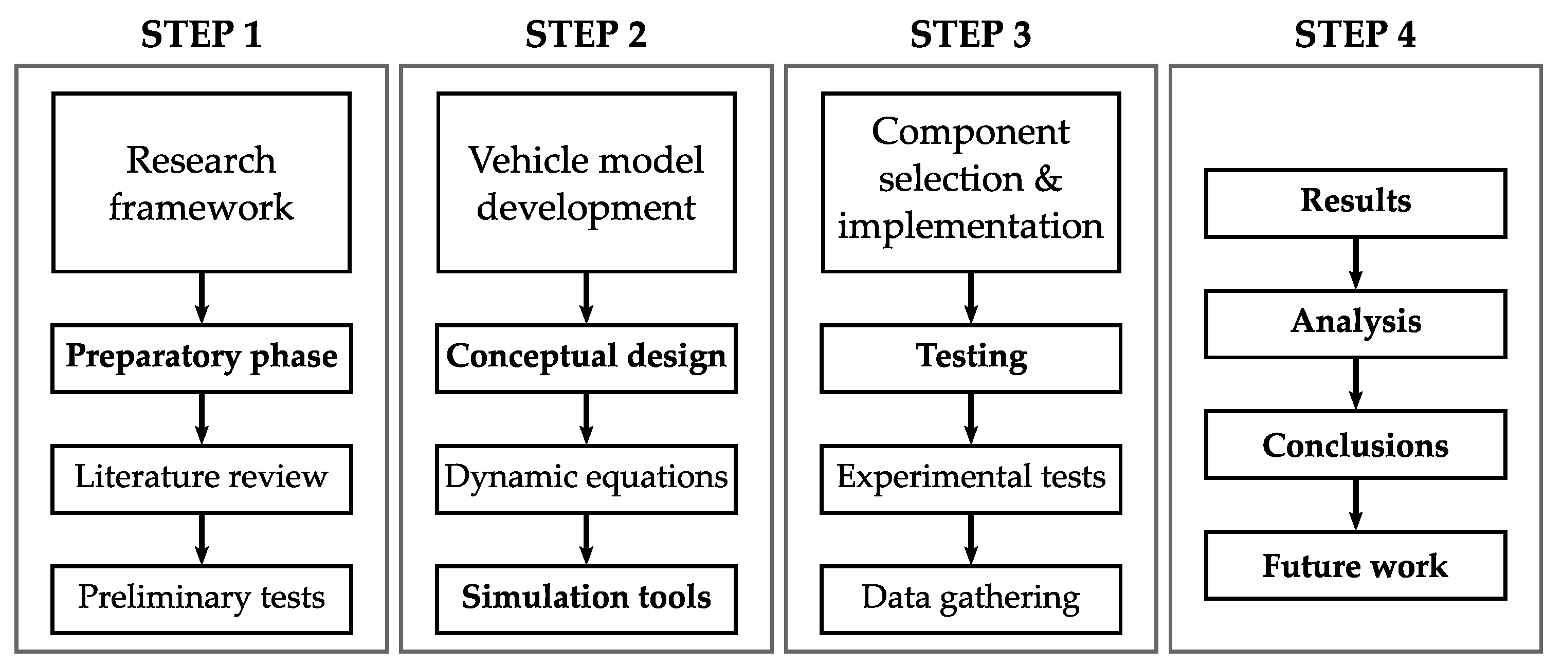
2. Proposed Methodology

The methodology to optimize the final ratio in an electric vehicle is shown in Figure 1. This methodology suits the project’s scope because it includes a preparatory phase, model vehicle development, selection, and implementation of components that improve the energy consumption and testing [23].

2.1. Test Setup

The testing protocol was carried out at the chassis dynamometer platform at the Automotive Mechatronics Research Center (CIMA in Spanish) laboratory of Tecnológico de Monterrey. In this test rig, a driving cycle speed profile is artificially reproduced on the vehicle. Simultaneously, relevant signals are acquired on the vehicle to verify its autonomy, energy consumed, acceleration, velocity, mechanical and electric power, among other meaningful quantities.

2.2. Physical Implementation

After integrating the mathematical models, different simulations are performed by varying the height profiles in the driving cycles and simulating different final ratios that could be used. Then select a final ratio and integrate it into the electric vehicle in a physical way.

2.3. Data Acquisition

For the data collection, we used the DEWESOFT hardware and software. These tools allow measuring the current and voltage in real-time when performing the different driving cycles.

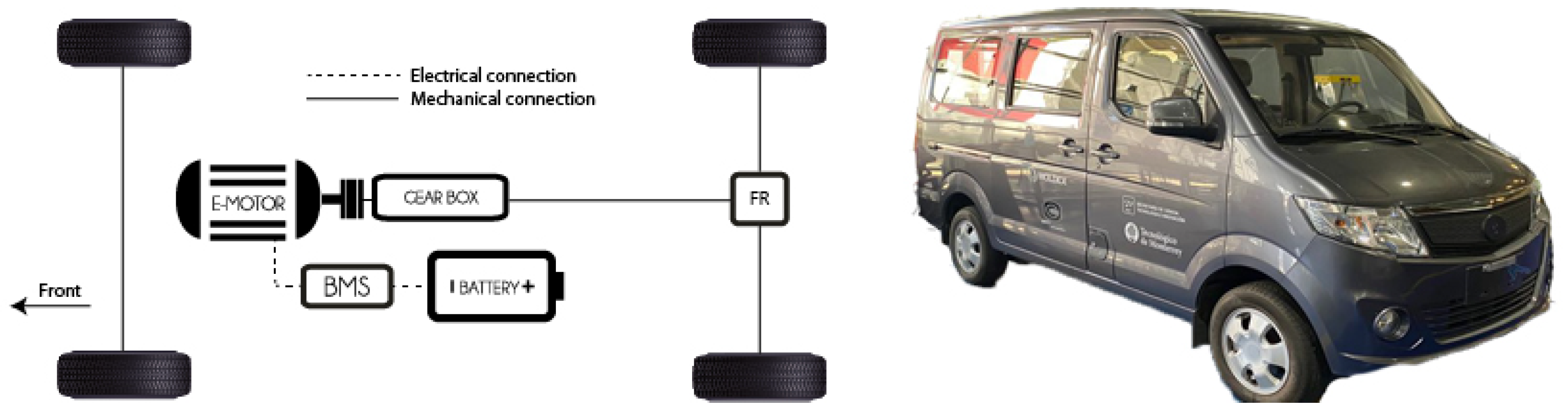
3. Experimental Test Vehicle

This work’s experimental platform is an electric vehicle (Van type) assembled in Mexico available at the Research Center or Automotive Mechatronics (CIMA), the electric vehicle called GMTA-E1, currently used as a cab in Mexico City. Using an electric configuration in a vehicle for public transportation reduces the emissions produced and emitted to the environment compared to internal combustion vehicles. Furthermore, a city vehicle maintains high efficiency at low revs, making it ideal for established work.

The powertrain consists of one central induction electric motor with nominal power of 15 hp. It has three phases and four poles, and it is mechanically coupled to a five-speed gearbox, which finally leads to a differential on the rear axle that delivers power to the wheels. The operating region of the electric motors ranges between 96 and 220 V. A 32-kW battery pack powers the electric motor. The platform configuration is shown in Figure 2.

The operation of the electric vehicle starts with the driver pressing the accelerator pedal. Depending on the throttle demand, a torque setpoint is requested for the induction machine power stage. This unit is a three-phase voltage inverter that ideally demands constant voltage and variable current to the battery management system (BMS). From an energy perspective, the electric motor transforms electrical energy into the mechanical domain. Its rotation is transferred through the gearbox into the differential. It finally reaches the rear wheels, thus yielding longitudinal vehicle motion. The characteristic curves of the induction motor are shown in Figure 3, where the torque and efficiency behavior are illustrated against the rotational speed. Full vehicle features are summarized in

Table 1. Vehicle features.

Description	Symbol	Unit	Value
Powertrain	−	−	Central electric motor with five-speed gearbox and final ratio
Vehicle mass	m	$\mathrm{kg}$	1370
Battery pack capacity	−	$\mathrm{kWh}$	32 (Li-ion cells)
Nominal voltage	$E_0$	$\mathrm{V}$	105
Maximum capacity	Q	$\mathrm{Ah}$	304
Initial state-of-charge	−	%	100
Internal resistance	$\mathrm{\Omega }$	$\mathrm{Ohms}$	0.07
Nominal current discharge	i	$\mathrm{A}$	160
Exponential voltage	$\alpha$	$\mathrm{V}$	106
Exponential capacity	$\beta$	$\mathrm{Ah}$	260
Frontal area	A	${\mathrm{m}}^2$	2.15
Drag coefficient	$C_d$	−	0.436
Rolling resistance coefficient	${\mu }_{rr}$	−	$0.015$
Gearbox efficiency	${\eta }_g$	−	0.95
First shift ratio	${ϵ}_{g,1}$	−	3.636
Second shift ratio	${ϵ}_{g,2}$	−	1.9641
Third shift ratio	${ϵ}_{g,3}$	−	1.428
Fourth shift ratio	${ϵ}_{g,4}$	−	1
Fifth shift ratio	${ϵ}_{g,5}$	−	0.801
Final ratio efficiency	${\eta }_d$	−	0.95
Final ratio	${ϵ}_d$	−	4.3
Maximum torque	−	$\mathrm{Nm}$	691.51
Maximum power	−	$\mathrm{kW}$	25.92
Maximum speed	−	$\mathrm{km}/\mathrm{h}$	117

. These parameters were obtained through dedicated characterization experiments using CIMA’s laboratory equipment, such as a chassis dynamometer.

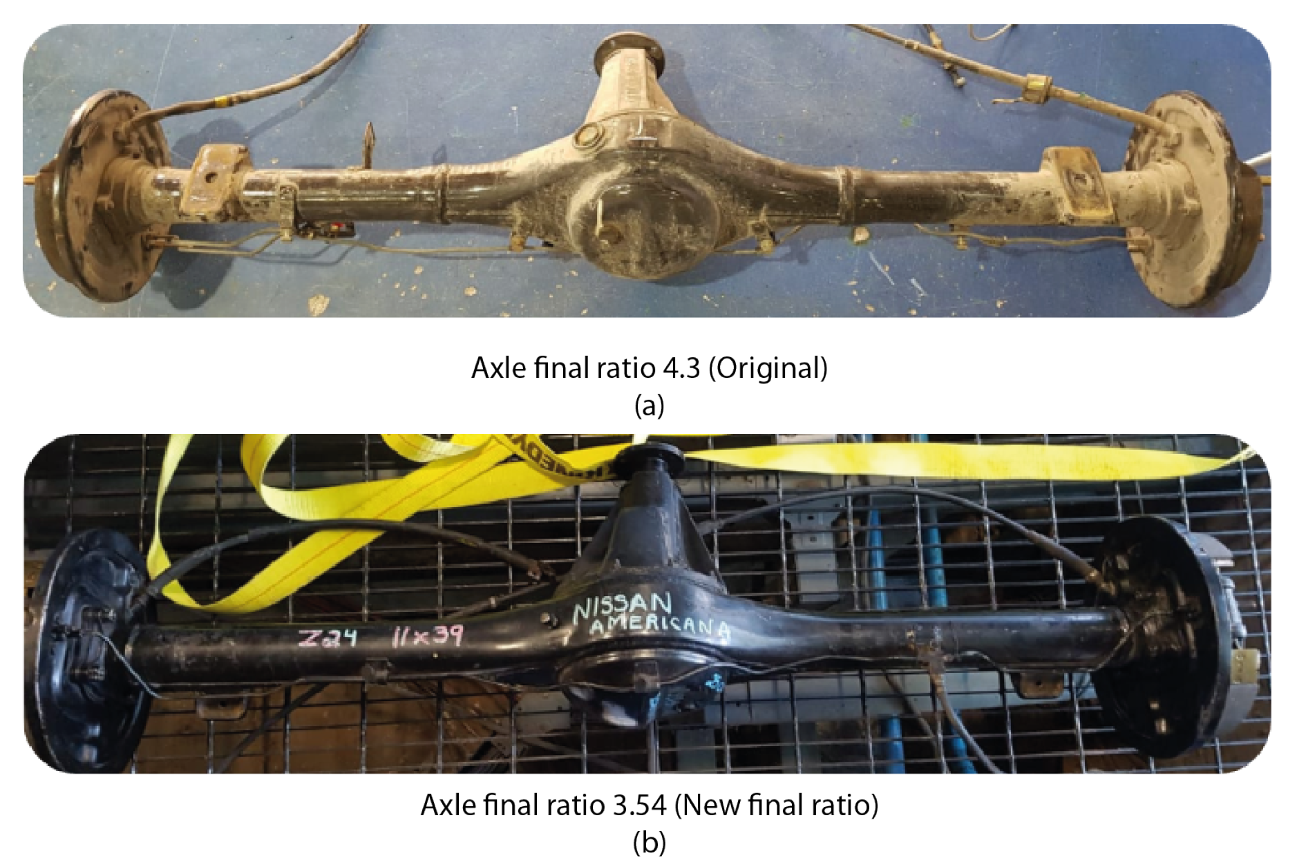
Physical Implementation of the New Differential Final Ratio

The final differential ratio is changed after proving that a lower final differential ratio improves the consumption and performance of the electric vehicle. However, manufacturing and cost constraints hindered the development of a dedicated prototype. Specifically, the development of a prototype cone and differential crown and the manufacturing process was very high. Therefore, developing a prototype without considering mass production in the future was not profitable, even more, when considering the lack of machinery to manufacture helical gears.

For this reason, we searched the market for an axle with a final differential ratio lower than 4.3, as this improves energy efficiency according to the simulations. Thus, an axle with a final ratio of 3.54 was implemented in the electric vehicle. Therefore, the only change was the final differential final ratio; the vehicle’s weight remained constant and the tire’s dynamic radius. A comparison between original and new axles is depicted in Figure 4.

4. Modeling

This section describes the mathematical tools used to represent vehicle dynamics and battery behavior.

4.1. Vehicle Dynamics

The longitudinal dynamics of the vehicle account only for throttle or brake control actions; vertical, lateral, and roll dynamics are neglected. The force that moves the car forward must overcome the following effects:

• Rolling resistance
• Aerodynamic drag
• Vehicle weight when running through a graded road
• Inertial forces whenever a change in velocity is required

This situation is depicted in the free-body diagram of Figure 5. In the following, we describe each contribution together with the tests performed to identify relevant parameters.

4.1.1. Rolling Resistance Force

This force is due to the friction of the vehicle tire on the road. It is expressed as:

$$F_{rr}={\mu }_{rr}mg$$

(1)

where ${\mu }_{rr}$ is the rolling resistance coefficient, m is the vehicle mass and $g=9.81\mathrm{m}/{\mathrm{s}}^2$ is the gravity acceleration. In this case, we followed the guidelines established by the International Organization for Standardization (ISO) for the experimental calculation of ${\mu }_{rr}$ [24].

4.1.2. Aerodynamic Drag

This force is due to the friction of the vehicle’s body moving through the air. It is given by:

$$F_{ad}=\frac{1}{2}\rho A{C}_d{v}^2$$

(2)

Here, $\rho =1.225\mathrm{kg}/{\mathrm{m}}^3$ is the density of the air, $C_d$ is the aerodynamic drag coefficient, A is the frontal area of the vehicle, and v is its longitudinal speed. In this case, $C_d$ was obtained through computational fluid dynamics (CFD) simulations, whereas A was quantified with vehicle dimensions.

4.1.3. Hill Climbing Force

This term denotes the force needed to drive the vehicle up through a graded road:

$$F_{hc}=mg\sin \psi$$

(3)

where $\psi$ is the angle of the road slope.

4.1.4. Net Force

The vehicle’s acceleration can then be computed using Newton’s second law after determining the net thrust of the car as a function of speed. Noticing that vehicle’s translational motion is coupled to the rotational movement of the components connected with the wheels, including the engine and the driveline. Any change of translational speed will therefore be accompanied by a corresponding shift in the rotational speed of the components coupled to the wheels. Therefore, mass factor ${\gamma }_m$ is introduced into the following equation to calculate the vehicle acceleration a [25]. Thus, it takes into account the effect of the inertia of the rotating parts on vehicle acceleration characteristics. The resulting equation is:

$$F_{net}={\gamma }_{m}ma$$

(4)

The mass factor ${\gamma }_m$ can be determined from the moments of inertia of the rotating parts, i.e., wheels, gearbox gears, and differential. For example, for passenger cars, the mass factor may be calculated using the following relation:

$${\gamma }_m=1.04+0.0025{\left({ϵ}_g{ϵ}_d\right)}^2$$

(5)

The first term on the right-hand side of Equation (5) represents the contribution of the rotating inertia of the wheels. In contrast, the second term means the contribution of the inertia of the components rotating at the equivalent engine speed with the overall gear reduction. Thus, ${ϵ}_g$ indicates the gearbox ratio, whereas ${ϵ}_d$ denotes the differential or final ratio.

4.1.5. Tractive Force

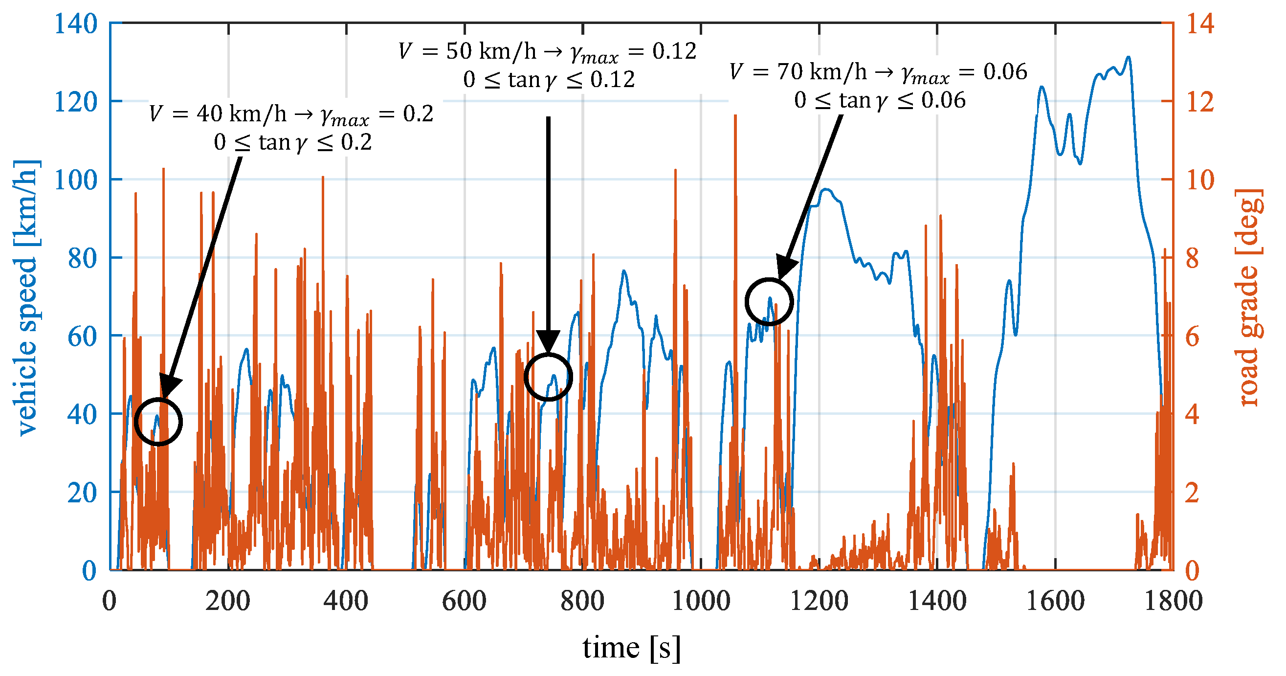
The tractive force is calculated by summing the force mentioned above contributions:

$$F_t=F_{net}+F_{hc}+F_{ad}+F_{rr}$$

(6)

Consequently, the tractive force is converted into power as follows:

$$P_m=F_{t}v$$

(7)

4.1.6. Gradability

Gradability is usually defined as the maximum grade a vehicle can negotiate at a given steady speed. On a slope at a constant speed, the tractive effort has to overcome grade resistance, rolling resistance, and aerodynamic resistance. For a relatively small angle of $\psi$, $\tan \psi \approx \sin \psi$. Thus, when solving for $\psi$ from the Equation (3), we obtain:

$${\psi }_{max}=\arcsin \left(\frac{P_m{\eta }_t}{mgv}-\frac{\rho A{C}_d{v}^2}{2mg}-{\mu }_{rr}-\frac{{\gamma }_{m}a}{g}\right)$$

(8)

where, ${\psi }_{max}$ is the maximum grade of the road that the vehicle can overcome, $P_m$ is the engine power, and ${\eta }_t$ is the drivetrain efficiency.

4.2. Battery Model

The battery, a Li-ion cell pack, is described through its state of charge $SOC$, which quantifies its energy. $SOC=1$ denotes a fully charged battery. By converse, the battery is fully depleted at $SOC=0$. Energy flowing in (charge, $f_c$) or out (discharge, $f_{dc}$) is calculated at every time step of a driving as follows:

$$\begin{array}{cc}\hfill f_{dc}& =E_0-K\frac{Q}{Q-it}{i}^{*}-K\frac{Q}{Q-it}it+\alpha e^{-\beta it}\hfill \end{array}$$

(9)

$$\begin{array}{cc}\hfill f_c& =E_0-K\frac{Q}{it+0.1Q}{i}^{*}-K\frac{Q}{Q-it}it+\alpha e^{-\beta it}\hfill \end{array}$$

(10)

In these expressions, t is the time, $E_0$ is the nominal voltage, K is the polarization constant, i is the battery current, $i^{*}$ is the current filtered with a low-pass filter ($\tau =10\mathrm{s}$), Q is the maximum battery capacity, $\alpha$ is the exponential voltage and $\beta$ is the exponential capacity.

5. Simulations

A numerical model can calculate the power required for traction while the vehicle is moving on the road. This traction power is directly proportional to the force exerted by the electric motor. For vehicle model calculations, the following assumptions hold:

• The vehicle moves only in the longitudinal direction.
• The system is considered as ideally rigid; no vibration or damping effects are accounted for.
• The tire radius is assumed to be constant.

A backward vehicle model was built and tested using MATLAB/Simulink^®. The Figure 6 shows the general block diagram of the model, starting from the speed profile given by the driving cycle, which reaches the block where the required mechanical power is calculated. Next, the model is complemented by calculating significant contributions that oppose the vehicle’s movement and transform quantities through the gearbox’s ratios and the differential. Next, electrical to mechanical conversion takes place in the electric motor, whose efficiency is accounted for. Finally, the induction machine demands variable current profiles according to the traction request in the electrical domain; the way to find the energy consumption is done by solving all equations with respect to time. The time is the time it takes to perform the driving cycle.

In this context, using a backward model works under the hypothesis that the vehicle can reproduce all the speed points in the input profile. The idea should hold true when simulating standardized driving cycles, as in this case. One benefit of this approach is that the simulation takes a significantly lower amount of resources when compared to forward models [26].

5.1. Driving Cycles

Driving cycles are a collection of variable longitudinal velocity setpoints in time. In the context of electric vehicles, driving cycles play a fundamental role in determining energy consumption and, ultimately, vehicle autonomy. In this particular research, we used three common cycles to explore energy consumption: the new European driving cycle (NEDC), worldwide harmonized light vehicle test cycle type 2 (WLTC-2), and type 3 (WLTC-3) [27,28,29].

The driving cycle constitutes the main input of the described model. Furthermore, it denotes acceleration, speed, and traveled distance for the vehicle. With these cycles, simulations were carried out under different circumstances.

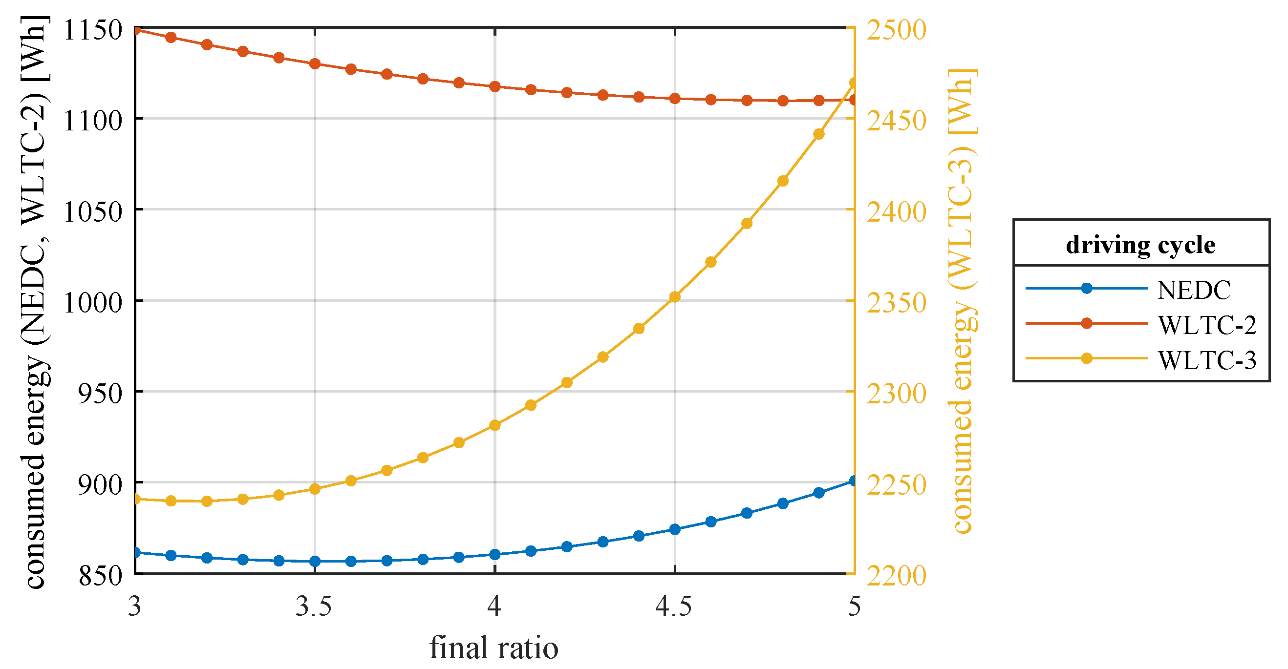
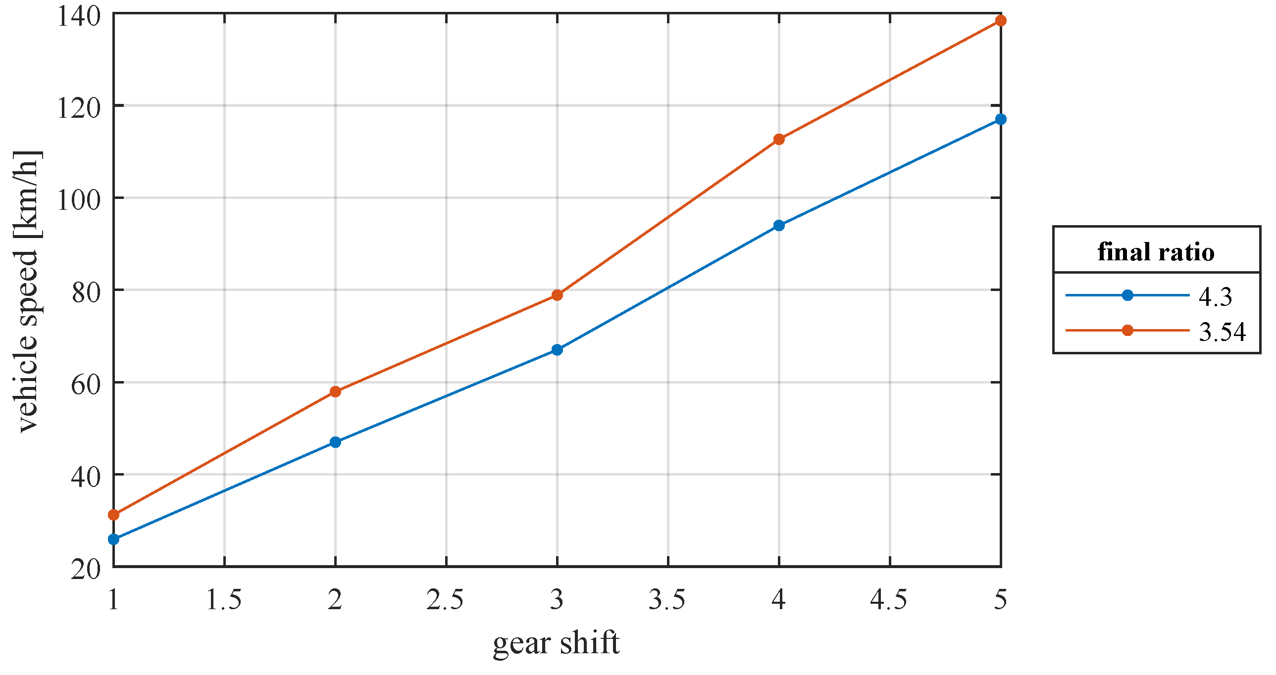
5.2. Final Ratio Influence

Results in Figure 7 demonstrate that, except for the WLTC-2 cycle, lower final ratios involve lower energy consumption. For example, the final ratio of the original differential of the electric vehicle is 4.3. Thus, we could attain a more efficient operation by selecting a differential with a lower final ratio.

The state of charge is inversely related to the energy consumed. With a traveled distance of 27 km and a maximum speed of 127 km/h, the WLTC-3 cycle depletes the battery faster than the NEDC or WLTC-2 cycles. Starting with a full battery, $SOC=91\%$ is attained after the WLTC-3 cycle. In contrast, $SOC=95.99\%$ and $SOC=96.36\%$ for NEDC and WLTC-2 cycles, respectively.

6. Experimental Validation

We consider as maximum speed the speed that the vehicle can reach with a specific gearbox shift. With the aid of the chassis dynamometer, we measured vehicle speed for each shift with both differential axles. From Figure 8, a significant change can be observed for the final vehicle speed for each shift. For example, with a final ratio of 4.3, the vehicle could only reach 117 km/h, and with the new final ratio of 3.54, it can reach 139 km/h, which means an increase in speed of 16%.

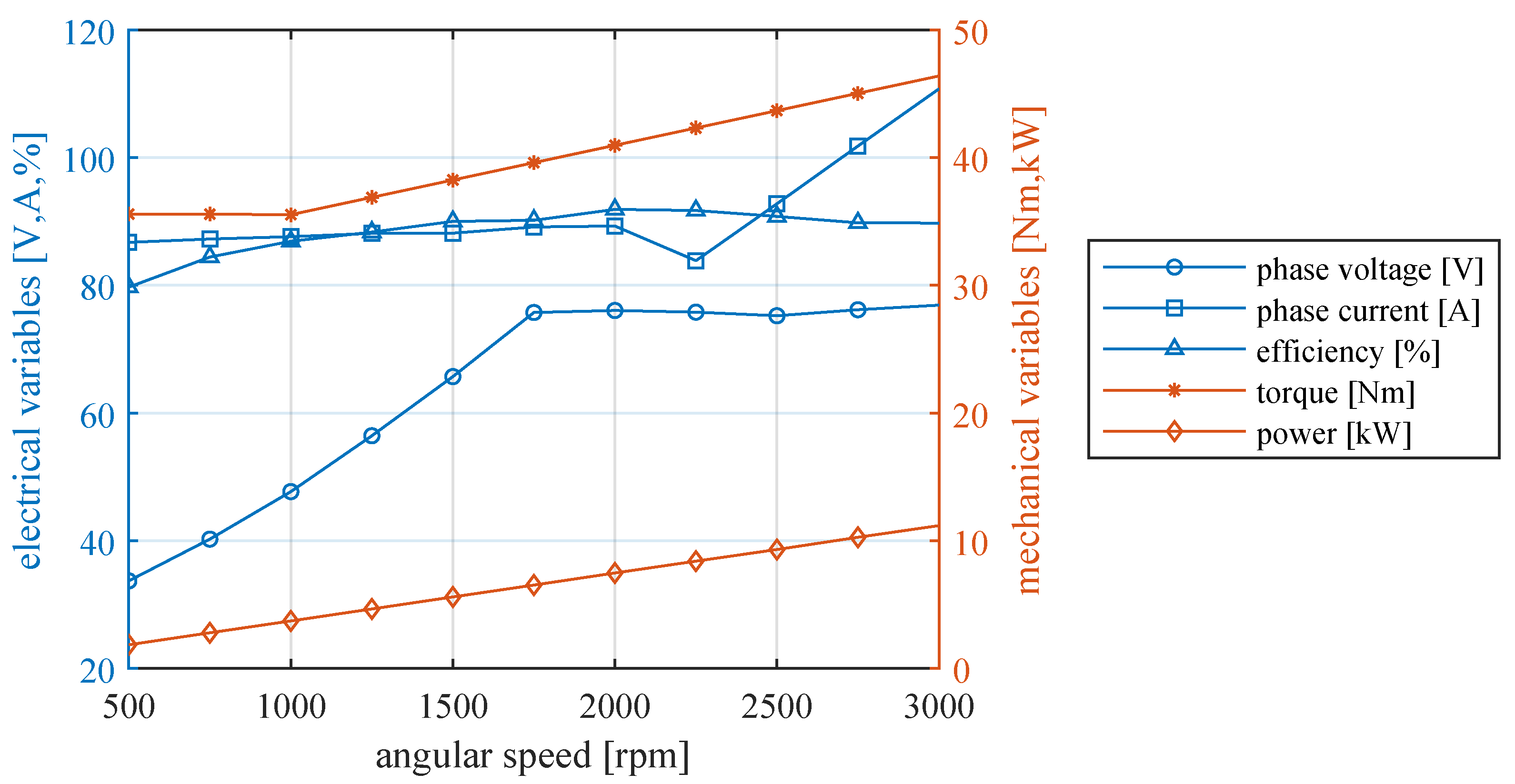
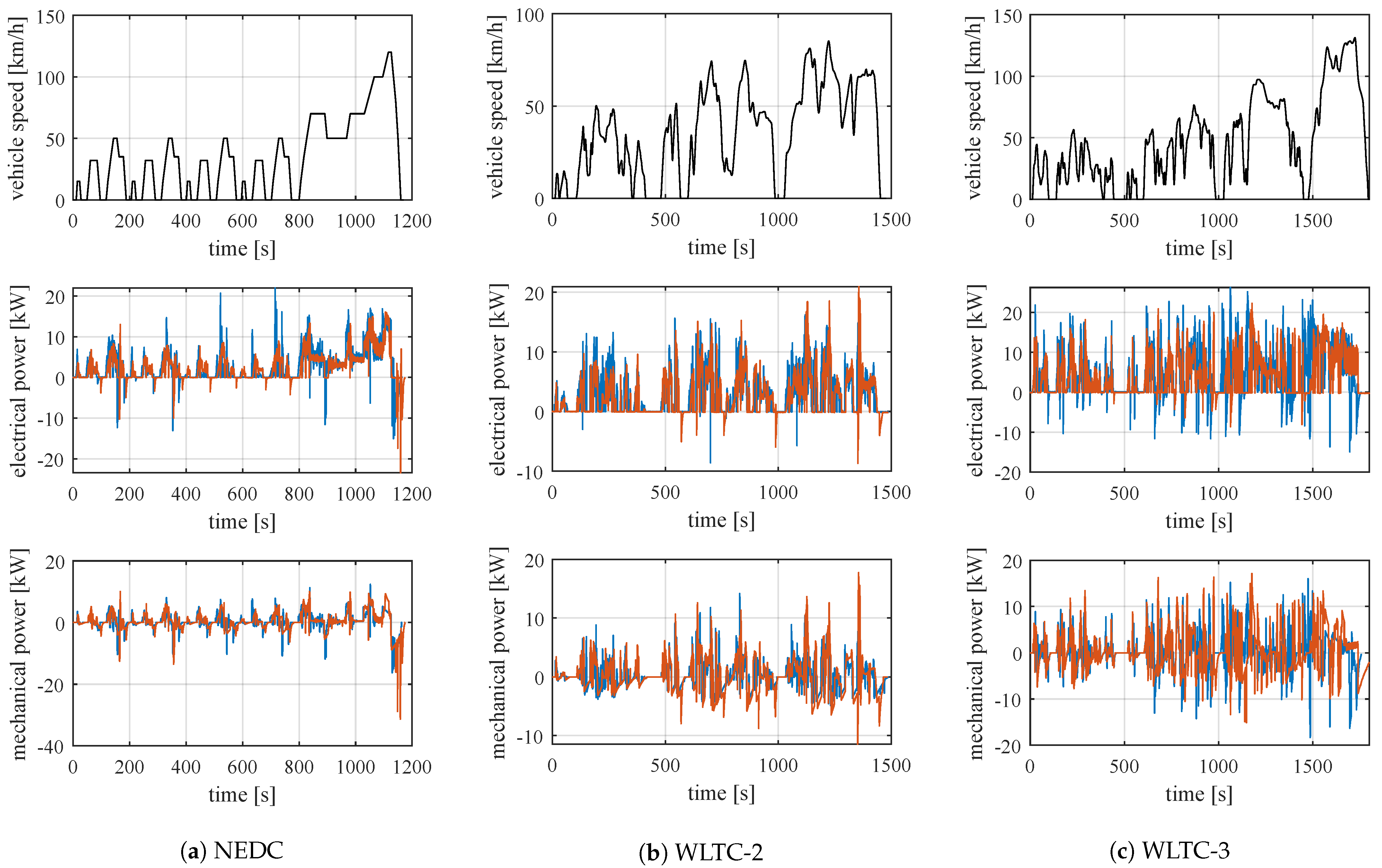
6.1. Electric and Mechanical Power Delivered by the Vehicle

As mentioned in the developed model, testing was performed through the NEDC, WLTC-2, and WLTC-3 standardized driving cycles while applying final ratios of 4.3 and 3.54. For the experiments, We reproduced these cycles on the chassis dynamometer. The first row of Figure 9 shows the time histories of the cycles mentioned. The speed profile is followed in each case, and the mechanical and electrical power values were recorded over the time.

The measured electrical power was extracted from the battery pack using the DEWESOFT equipment. In turn, mechanical energy is measured at the wheels using the chassis dynamometer. Electrical power results generally show higher consumption when using a ratio of 4.3, as shown in Figure 9. In contrast, mechanical power numbers exhibit less abrupt variations among the different ratios.

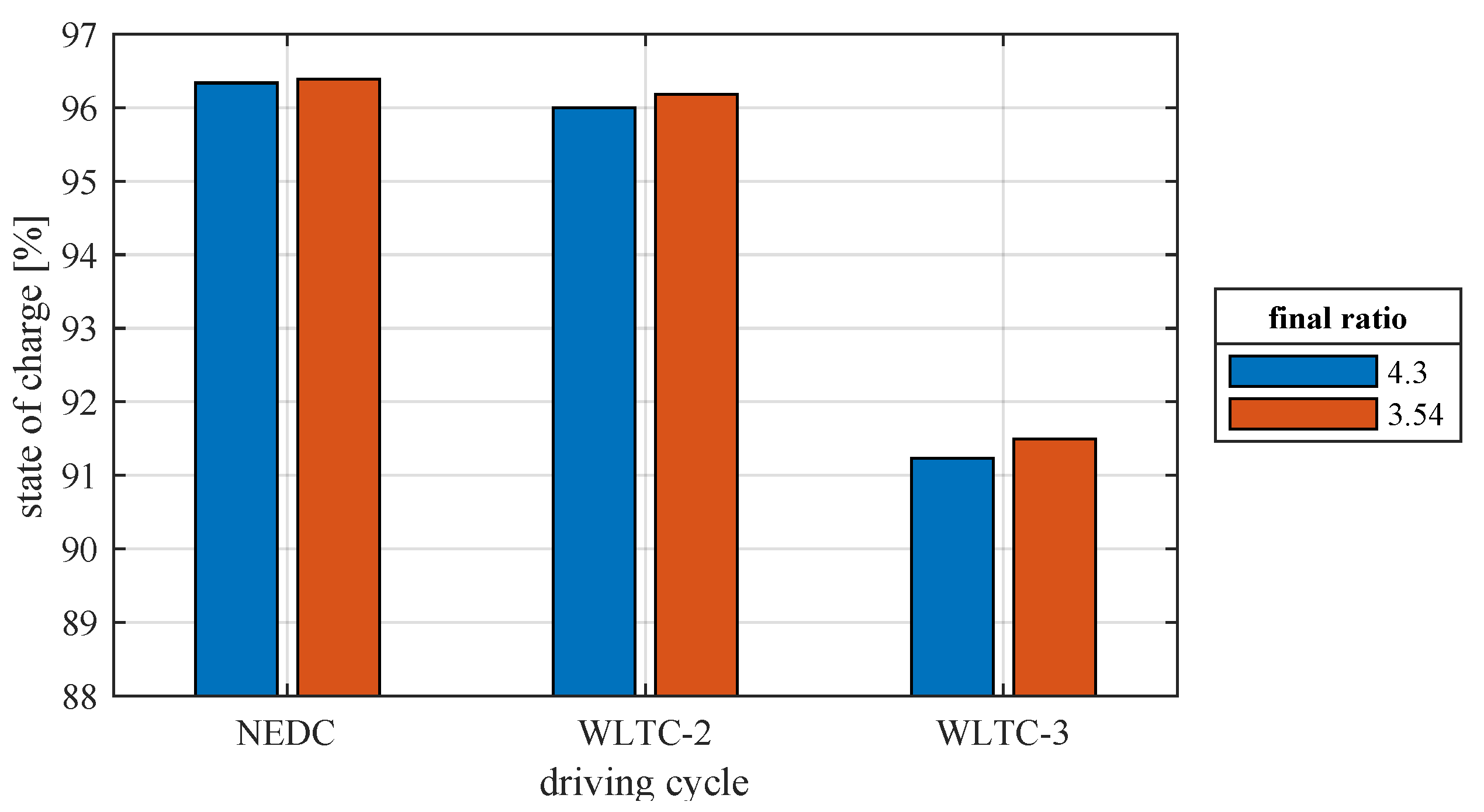
6.2. Energy Management Test Simulation

To compare the energy consumed with the two differential ratios, we run our model developed in MATLAB/Simulink^®, thus obtaining the bar plot shown in Figure 10. These results indicate that, for every driving cycle, the state of charge is superior when using a ratio of 3.54, as anticipated by the simulations.

7. Results and Discussion

7.1. Road Grade Influence

The electric vehicle tested has a five-speed gearbox. Each gear transmits power with a specific ratio to accelerate the vehicle and overcome eventual variations of road slope. Thus, to analyze the influence of road grade on energy consumption, we randomly generated 80-grade profiles.

First, depending on the running speed, we selected the polynomial equation of the characteristic curve of the motor at that speed gearbox. Next, the angle ${\psi }_{max}$ was calculated at every time instant using Equation (8). Then, an angle $\psi$ is randomly assigned, such that $0\le \psi \le {\psi }_{max}$. For this specific case, the WLTC-3 driving cycle was used, as shown in Figure 11.

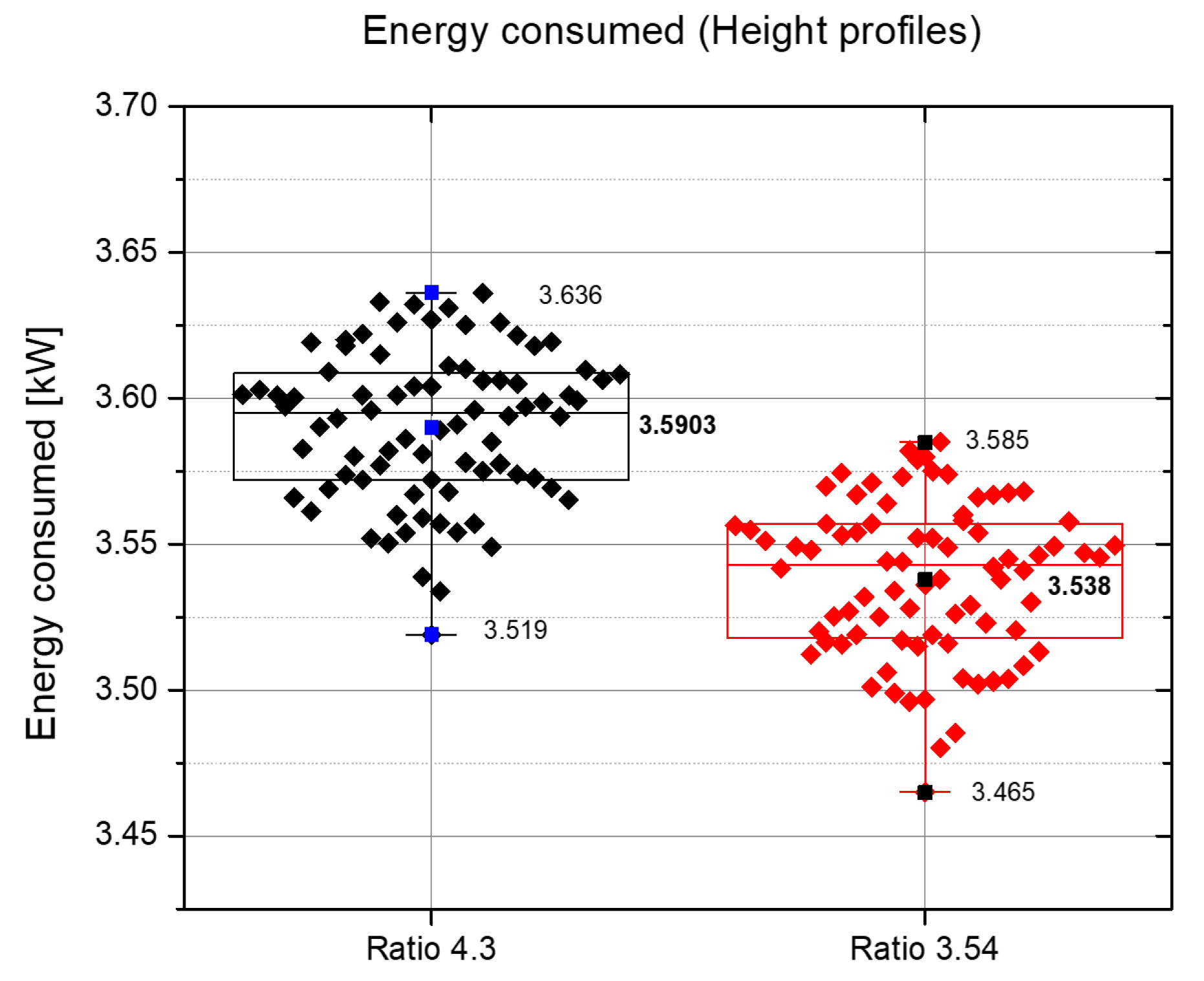
7.2. Energy Consumed Simulated with Height Profiles

We ran 160 simulations for the energy consumption analysis, the first 80 with a final ratio of 4.3 and the remaining ones with a final ratio of 3.54 using various height profiles. The results are shown in Figure 12. The results indicate that energy consumption values are lower using the final 3.5 ratio than the original 4.3 ratio. We ran 160 simulations for the energy consumption analysis, the first 80 with a final ratio of 4.3 and the remaining ones with a final ratio of 3.54 using various height profiles. The results are shown in Figure 12. The results indicate that energy consumption values are lower using the final 3.5 ratio than the original 4.3 ratio.

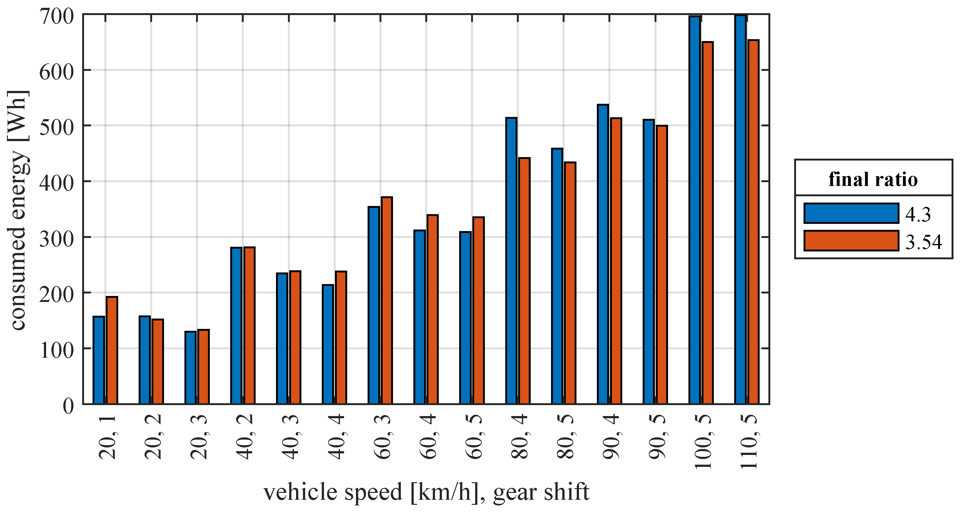
7.3. Energy Consumed at a Constant Speed

The energy consumed in one minute is shown in Figure 13, summarizing that the test was performed at different constant speeds and in different speeds gearbox. As can be seen, at low speeds, the energy consumption is similar. Still, the energy consumption is lower at high speeds, with the final ratio of 3.5 concerning the original final ratio of 4.3.

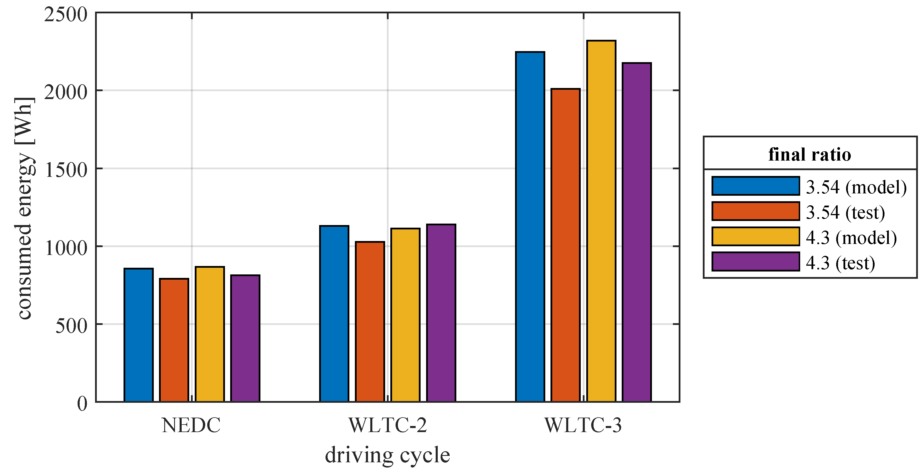
7.4. Energy Consumed in Driving Cycles

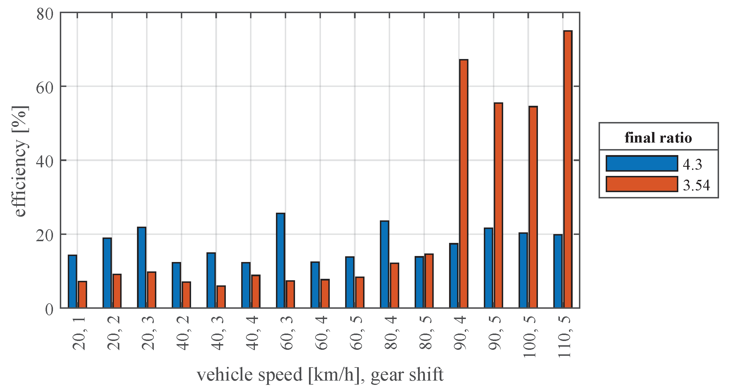
To validate the developed model, we first analyze the energy consumed in each cycle with a final ratio of 4.3. Figure 14 illustrates this comparison, which shows a minimum discrepancy between model and experiment of $-2.39\%$ for the WLTC-2 cycle. By converse, a maximum relative difference of $+6.66\%$ is found for the NEDC profile.

When analyzing the lower ratio of 3.54, the lowest discrepancy is $+8.29\%$ for the NEDC case, whereas the largest variation is found with WLTC-3: $+11.77\%$.

When comparing the experimental results between both final ratios, the lower final ratio of 3.54 always involves an adavantage in terms of consumed energy; with savings ranging from $10.76\mathrm{Wh}$ (NEDC) to $72.5\mathrm{Wh}$ (WLTC-3). These figures represent an energy increase on the original ratio configuration of $+2.81\%$ and $+8.28\%$, respectively.

7.5. Efficiency

We measured the electrical and mechanical power for one minute to determine the efficiency, the ratio between the electrical power demanded from the batteries, and the mechanical power delivered to the wheels. So for this test, we followed the same procedure in several gearbox speed changes to observe the efficiency variation and how it behaves. The vehicle can go at 20 km/h in first, second, and third gears. At 40 km/h in second, third, and fourth gears. At 60 km/h in third, fourth, and fifth gears. At 80 km/h in fourth and fifth gears. At 90 km/h in fourth and fifth gears. At 100 km/h in fifth gear and 110 km/h in fifth gear.

The efficiency is shown in Figure 15; at low speeds, the efficiency is higher with the final ratio of 4.3, but once the speed increases, the final ratio of 3.54 still increases its efficiency. Efficiencies above 60% are obtained when exceeding 80 km/h. While at speeds below 60 km/h, the efficiencies do not exceed 30% at 110 km/h, the efficiency of the entire powertrain is 75%, which is the maximum efficiency found in the vehicle.

8. Conclusions

This document shows a methodology for developing the dynamic model and optimization of the powertrain of an electric vehicle. This model allows the simulation of an electric vehicle and, through that simulation, obtain an ideal differential ratio for the different standardized driving cycles. The purpose is to help in reducing energy consumption, especially for converted vehicles.

Using a short differential ratio, 3.54 benefits the maximum final speed in the electric vehicle. However, this change does not affect the electric motor’s high efficiency, torque, and power, being opposite of what is seen in an internal combustion vehicle, where short differential ratios are used just in high-power power engines.

The ratio change from 4.3 to 3.54 in the differential directly influences energy saving according to the performed energy analysis. For the handling cycles used in this study, savings variated between 3% and 8% at the system level.

A more efficient system directly impacts vehicle energy consumption. Furthermore, this improvement yields a reduction of mechanical wear, electrical loadings, and battery pack cycling, thus ensuring a longer lifespan in all the relevant domains of interest.

Further developments of this work could involve the optimization of the powertrain at a system level, i.e., accounting for the electric motor, gearbox, and differential systems under the same procedure. In addition, this analysis could be extended for hybrid vehicles, where the interaction with the internal combustion engine yields a more complex system to assess.

References

1. Yang, S.S.; Chong, Z. Smart city projects against COVID-19: Quantitative evidence from China. Sustain. Cities Soc. 2021, 70, 102897. [Google Scholar] [CrossRef]
2. Thornbush, M.; Golubchikov, O. Smart energy cities: The evolution of the city-energy-sustainability nexus. Environ. Dev. 2021, 39, 100626. [Google Scholar] [CrossRef]
3. Puma-Benavides, D.S.; Izquierdo-reyes, J.; Calderon-najera, J.D.D.; Ramirez-mendoza, R.A. A Systematic Review of Technologies, Control Methods, and Optimization for Extended-Range Electric Vehicles. Appl. Sci. 2021, 11, 7095. [Google Scholar] [CrossRef]
4. Chan, C.C. The state of the art of electric and hybrid vehicles. Proc. IEEE 2002, 90, 247–275. [Google Scholar] [CrossRef] [Green Version]
5. Tesla Company. Model S Owner’s Manual; Tesla Company: Palo Alto, CA, USA, 2019. [Google Scholar]
6. Tesla Company. Model X Owner’s Manual; Tesla Company: Palo Alto, CA, USA, 2018. [Google Scholar]
7. General Motors. 2019 Chevrolet Volt Brochure; General Motors: Detroit, MI, USA, 2018. [Google Scholar]
8. Krasopoulos, C.T.; Beniakar, M.E.; Kladas, A.G. Velocity and torque limit profile optimization of electric vehicle including limited overload. IEEE Trans. Ind. Appl. 2017, 53, 3907–3916. [Google Scholar]
9. Wu, G.; Zhang, X.; Dong, Z. Impacts of Two-Speed Gearbox on Electric Vehicle’S Fuel Economy and Performance; Technical Report, SAE Technical Paper; SAE International: Warrendale, PA, USA, 2013. [Google Scholar]
10. Hofstetter, M.; Lechleitner, D.; Hirz, M.; Gintzel, M.; Schmidhofer, A. Multi-objective gearbox design optimization for xEV-axle drives under consideration of package restrictions. Forsch. Ingenieurwesen 2018, 82, 361–370. [Google Scholar]
11. Nemeth, T.; Bubert, A.; Becker, J.N.; De Doncker, R.W.; Sauer, D.U. A simulation platform for optimization of electric vehicles with modular drivetrain topologies. IEEE Trans. Transp. Electrif. 2018, 4, 888–900. [Google Scholar]
12. Kabalan, B.; Vinot, E.; Trigui, R.; Dumand, C. Systematic methodology for architecture generation and design optimization of hybrid powertrains. IEEE Trans. Veh. Technol. 2020, 69, 14846–14857. [Google Scholar]
13. Schiffer, S.; Kain, A.; Wilde, P.; Haber, J.; Helbing, M.; Baeker, B. Influence of the final drive ratio on the consumption of passenger cars under real driving conditions. In Proceedings of the 2017 12th International Conference on Ecological Vehicles and Renewable Energies (EVER 2017), Monte Carlo, Monaco, 11–13 April 2017; pp. 1–11. [Google Scholar] [CrossRef]
14. Miller, J.M. Hybrid electric vehicle propulsion system architectures of the e-CVT type. IEEE Trans. Power Electron. 2006, 21, 756–767. [Google Scholar] [CrossRef] [Green Version]
15. Kim, N.; Cha, S.W.; Peng, H. Optimal Equivalent Fuel Consumption for Hybrid Electric Vehicles. IEEE Trans. Control Syst. Technol. 2012, 20, 817–825. [Google Scholar] [CrossRef]
16. Tang, X.; Yang, W.; Hu, X.; Zhang, D. A novel simplified model for torsional vibration analysis of a series-parallel hybrid electric vehicle. Mech. Syst. Signal Process. 2017, 85, 329–338. [Google Scholar] [CrossRef]
17. Prajwal, C.P.; Rao, K.U.; Hegde, K.R.; Nagaraj, S. A simple novel algorithm to optimize final gear ratio in electric and hybrid formula racing cars. In Proceedings of the 2013 IEEE International Multi Conference on Automation, Computing, Control, Communication and Compressed Sensing (iMac4s 2013), Kottayam, India, 22–23 March 2013; pp. 415–419. [Google Scholar] [CrossRef]
18. Naunheimer, H.; Bertsche, B.; Ryborz, J.; Novak, W. Automotive Transmissions; Springer: Berlin/Heidelberg, Germany, 2011. [Google Scholar] [CrossRef]
19. Hofman, T.; Dai, C.H. Energy efficiency analysis and comparison of transmission technologies for an electric vehicle. In Proceedings of the 2010 IEEE Vehicle Power and Propulsion Conference (VPPC 2010), Lille, France, 1–3 September 2010. [Google Scholar] [CrossRef]
20. Ding, X.; Guo, H.; Xiong, R.; Chen, F.; Zhang, D.; Gerada, C. A new strategy of efficiency enhancement for traction systems in electric vehicles. Appl. Energy 2017, 205, 880–891. [Google Scholar] [CrossRef]
21. Julio-Rodríguez, J.D.C.; Santana-Díaz, A.; Ramirez-Mendoza, R.A. Individual Drive-Wheel Energy Management for Rear-Traction Electric Vehicles with In-Wheel Motors. Appl. Sci. 2021, 11, 4679. [Google Scholar] [CrossRef]
22. Liu, K.; Yamamoto, T.; Morikawa, T. Impact of road gradient on energy consumption of electric vehicles. Transp. Res. Part D Transp. Environ. 2017, 54, 74–81. [Google Scholar] [CrossRef]
23. Birkhofer, H. The Future of Design Methodology; Springer: New York, NY, USA, 2011. [Google Scholar]
24. ISO. Passenger Car, Truck and Bus Tyre Rolling Resistance Measurement Method—Single Point Test and Correlation of Measurement Results; ISO 28580:2018; ISO: Geneva, Switzerland, 2018. [Google Scholar]
25. Wong, J.Y. Theory of Ground Vehicles; Wiley-Interscience: Hoboken, NJ, USA, 2001; p. 528. [Google Scholar]
26. Mohan, G.; Assadian, F.; Longo, S. Comparative analysis of forward-facing models vs. backwardfacing models in powertrain component sizing. In Proceedings of the IET Hybrid and Electric Vehicles Conference 2013 (HEVC 2013), London, UK, 6–7 November 2013; IET: London, UK, 2013; pp. 1–6. [Google Scholar]
27. Analysis, U.E.; Learning, M.; Sizing, B. Applied Energy Energy Storage Sizing in Plug-in Electric Vehicles: Driving Cycle Uncertainty Effect Analysis and Machine Learning Based Sizing Framework. J. Energy Storage 2021, 41, 102864. [Google Scholar] [CrossRef]
28. Huzayyin, O.A.; Salem, H.; Hassan, M.A. A representative urban driving cycle for passenger vehicles to estimate fuel consumption and emission rates under real-world driving conditions. Urban Clim. 2021, 36, 100810. [Google Scholar] [CrossRef]
29. Kammuang-lue, N.; Boonjun, J. Energy consumption of battery electric bus simulated from international driving cycles compared to real-world driving cycle in Chiang Mai. Energy Rep. 2021, 7, 3267–3272. [Google Scholar] [CrossRef]
Figure 1. Optimization methodology of the final ratio.
Applsci 11 11474 g001
Figure 2. Platform configuration of a rear-wheel-drive electric vehicle with gearbox and differential (Final ratio FR) used in this work.
Applsci 11 11474 g002
Figure 3. Induction electric motor characteristic curves.
Applsci 11 11474 g003
Figure 4. Axles with (a) original final ratio (4.3), (b) new final ratio (3.54).
Applsci 11 11474 g004
Figure 5. The forces acting on the electric vehicle along a slope.
Applsci 11 11474 g005
Figure 6. Block diagram of the operation of the backward dynamic model for an electric vehicle in MATLAB/Simulink®.
Applsci 11 11474 g006
Figure 7. Final ratio influence carried out in the model simulations.
Applsci 11 11474 g007
Figure 8. Vehicle speed with final ratios of 4.3 and 3.54 for all the gear shifts.
Applsci 11 11474 g008
Figure 9. Electrical and mechanical power delivered by the battery and wheels, respectively, for NEDC, WLTC-2, and WLTC-3 driving cycles with final ratios of 4.3 (blue) and 3.54 (orange).
Applsci 11 11474 g009
Figure 10. State of charge in driving cycles model results with final ratios 4.3 and 3.54.
Applsci 11 11474 g010
Figure 11. Road grade profile generated during the WLTC-3 cycle.
Applsci 11 11474 g011
Figure 12. Energy consumed simulated with height profiles.
Applsci 11 11474 g012
Figure 13. Energy consumed at a constant speed.
Applsci 11 11474 g013
Figure 14. Energy consumed in driving cycles with final ratios 4.3 and 3.54. Model and test results are compared for both ratios.
Applsci 11 11474 g014
Figure 15. Efficiency at a constant speed.
Applsci 11 11474 g015