In this approach, in order to figure out the optimal antenna design which has the lowest
Cost corresponding to a set of design parameters, we employed a deep neural network (DNN) model to handle this regression task [
33]. The DNN model is a subfield of machine learning with algorithms inspired by the idea of simulating the human brain [
34]. The DNN model has recently gained increasing research interests due to their capability of overcoming the drawback of traditional algorithms dependent on hand-designed programs, and is investigated in many different domains, such as speech recognition, computer vision, pattern recognition, and regression [
35].
Besides, regression analysis is a statistical measurement for estimating the relationships between one dependent variable (the factor we want to understand or predict) and a series of independent variables (the factors that influence the dependent variable) [
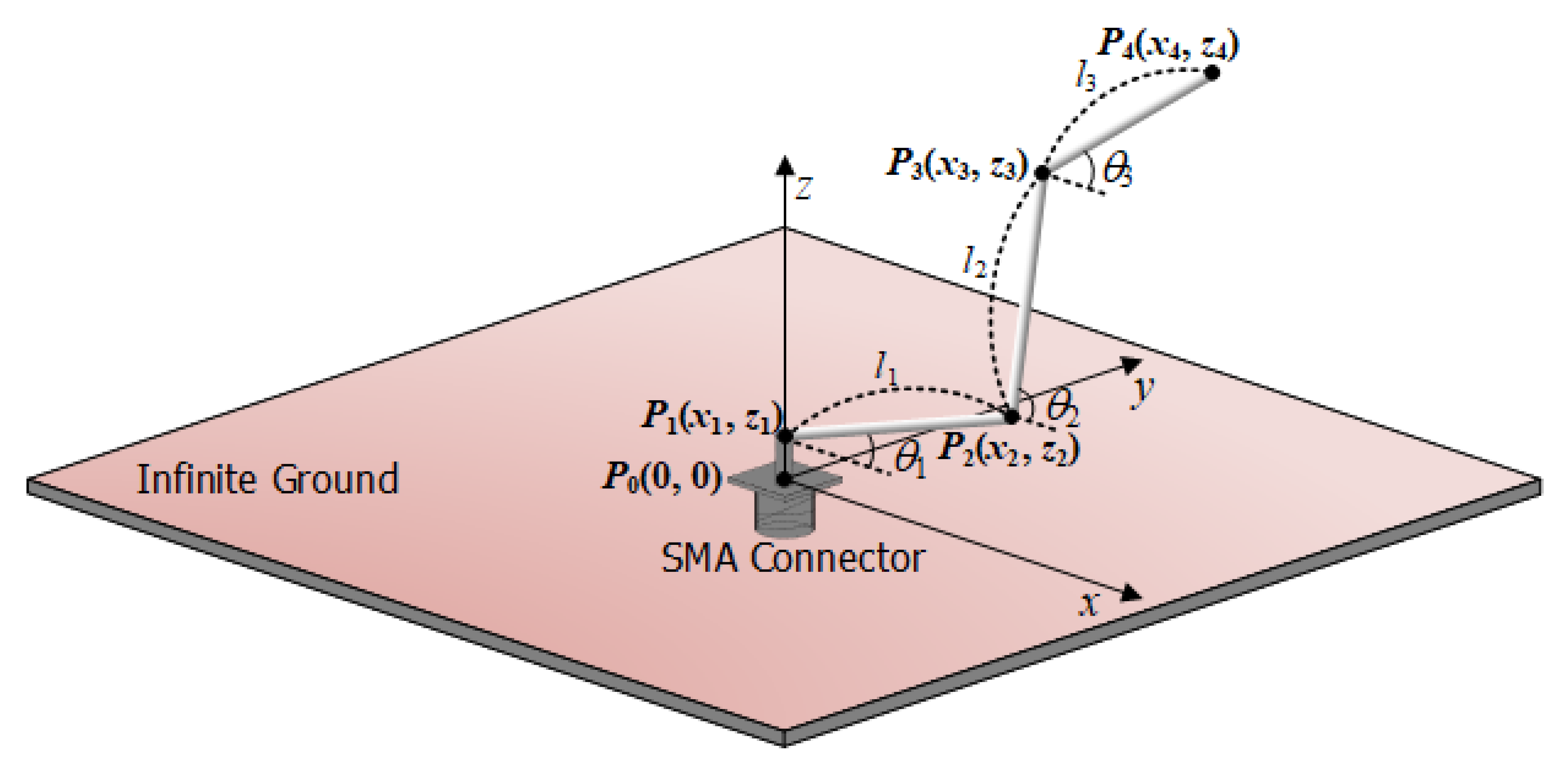
33]. Here, we propose a DNN model based on regression for the design of a bent wire monopole antenna. In this problem, the input variables are assigned as a set of six design parameters
X = {
l1, l2, l3, θ1, θ2, θ3} (expressed in
Section 2)
, and the output of the regression task is the corresponding output
y =
Cost as defined in (1). Therefore, the relation between the input and the output is formulated as:
where
F represents the DNN regression model including
a and
b as unknown parameters; the simple denotation for the complexity of the problem will be defined during the training process. In the training phase, mean squared error (
MSE) is utilized as the loss function [
36]. The
MSE is computed as the average of the squared differences between the predicted and actual
Cost values as:
where
n is represented for the number of data points, as well as
yi and
are the actual and the corresponding predicted
Cost values to the given design parameters
Xi, respectively. Minimizing the
MSE to zero is key for training the model because the
MSE approaching zero implies that the predicted
Cost is substantially similar to the actual
Cost computed from NEC simulation.
In addition, R-squared score (
R2) was chosen as a performance metrics to evaluate the model performance by comparing the trained model predictions with the observed data [
37,
38]. It is a statistical measure of how close the data are to the fitted regression line. The R-squared score is computed as:
where the unexplained variance is the sum of the square of the difference between the actual and predicted
Cost values and the total variance is calculated in a similar way by replacing the predicted value by the average actual one
.
We illustrated our machine learning process to predict the antenna design as a block diagram in
Figure 3. In this specific problem, the obtained data, which is composed of antenna design parameters and the
Cost value for each sample antenna, is used to train a machine learning model, or DNN. The model training process is discussed in detail in
Section 3.1. The remaining part of
Section 3 presents the plan to identify the optimal design parameters based on a grid search and the trained machine learning model as well as the performance verification.
3.1. Machine Learning Results
The data obtained in
Section 2.2 was fed into the DNN model with the proportion in percentage: training set/validation set/testing set = 70%/15%/15%. The training, validation, and testing sets make the specific roles in the machine learning process: all the samples in the training set are used for training the various models and the responsibility of the validation set is to compare their performances and choose which one to employ; on the other hand, the testing set is kept separately from the remaining to verify whether the final predictions of the trained model are correct or not. If the predictions tend to be distinct from the corresponding actual values, the training process needs to be reset.
Table 3 shows the structure of the proposed DNN model, where the activation functions are Rectified Linear Unit (ReLU) for hidden layers and linear for the final layer to generate the numerical output [
39,
40]. All these parameters are well defined for our dataset. The proposed model was trained using
MSE loss function, optimized by Adam [
41] with learning rate of 0.001 and batch size of 128. A set of sequential Dense layers—the basic layer which consumes the input and computes the new output by performing matrix-vector multiplications—is the main component of this network. Adding the dropout layer behind each Dense layer was considered due to its efficiency in preventing overfitting (a concept in data science that a model performs well on training data but tends to fail on the untrained data such as testing set; this is not the desired result for every type of model in machine learning). However, dropout regularization was claimed to be not well-performing in regression task as in classification and natural language processing tasks [
42]. Therefore, due to experiments, the dropout layer is not used in our model. The number of units in Dense layers are adjusted by trying multiple combinations to find the best preciseness for our dataset. The detailed information for the layers is summarized in
Table 3.
Figure 4 shows a comparison between the actual value and the predicted one in the testing set to visualize the performance of the proposed method. Each dot in the figure is formed by the numerical actual value as the
x-coordinate and the corresponding predicted values as the
y-coordinate. Therefore, if two values are more and more approximate, the point generated from them (the blue dots) will be closer and closer to the function graph
(the diagonal red line in the figure). Based on this figure, it could be argued that our prediction in testing phase is approaching the perfect performance, which confirms the efficiency of our DNN model.
Table 4 shows the comparison with two other machine learning techniques such as Lasso [
43] and Linear regression [
44].
MSE and R-squared score calculated on the testing set are utilized as the aspects of comparison. As mentioned before, smaller MSE and higher R-squared score denote a better model, therefore, our DNN model with
MSE of 0.0353 and R-squared score of 0.999 is superior to both Lasso and Linear regression. In the regression problem, the proposed DNN outperforms the other methods.
3.2. Validation of Machine Learning Model
To find the optimal design parameters of the bent wire antenna based on the proposed DNN model, a grid search is formed to the parameters l1, l2, l3, θ1, θ2, and θ3 with the number of points for each parameter double that of the one used for the training set while maintaining the range of each variable. This search ensures that this grid is denser than the training dataset. In other words, the number of points for each wire section length and each bending angle is 20 and 18, respectively. Therefore, the total number of samples generated by all possible combinations of parameters in this grid is 46,656,000.
All the samples in the grid are then put through our well-trained DNN model to obtain the corresponding
Cost value. To validate our ML model, we compared their
Costs derived from the ML model with those calculated by NEC simulation after extracting several designs of the antenna with
Costs of around 60, 70, and 80 from the grid search.
Table 5 represents the design parameters and corresponding
Costs derived from ML model and NEC simulation. The comparison of
Costs in
Table 5 reveals that the relative errors between
Costs from the ML model and NEC simulation are smaller than 2%, which verifies the accuracy of our ML model.
After searching the antenna models with high
AF on the entire grid using our ML model, we tabulated the design parameters and
AFs and
Costs of resulting antennas in comparison with the corresponding
AFs and
Costs derived by NEC simulations in
Table 6.
Table 6 shows the design parameters of the ranked antennas in terms of
AF/
Cost when searching the antenna models on the entire grid. The ranked antennas in
Table 6 achieve
AF over about 77%, which means the
Costs are smaller than about 46. In addition, the resulting
AFs from our ML model favorably agree with those from NEC simulation in that the maximum deviation between both
AFs for the same model is smaller than 1%. This agreement of the
AF indicates that our ML model is well-trained and capable of evaluating the impedance matching characteristic of a wire monopole antenna accurately.
The performed validation informs that the ML technique can be possibly applied to the antenna design from a practical standpoint. We thus expect that there may be a few advantages if the proposed method using ML technique is applied to antenna design. First, we can extract approximated optimal design parameters from the grid search using the ML model when beginning antenna design. Second, we can easily derive the key design parameters by analyzing the change of an evaluation function corresponding to a variation of an individual design parameter. Finally, we can expansively apply the proposed method using the ML technique to the design of antennas with a more complicated structure.
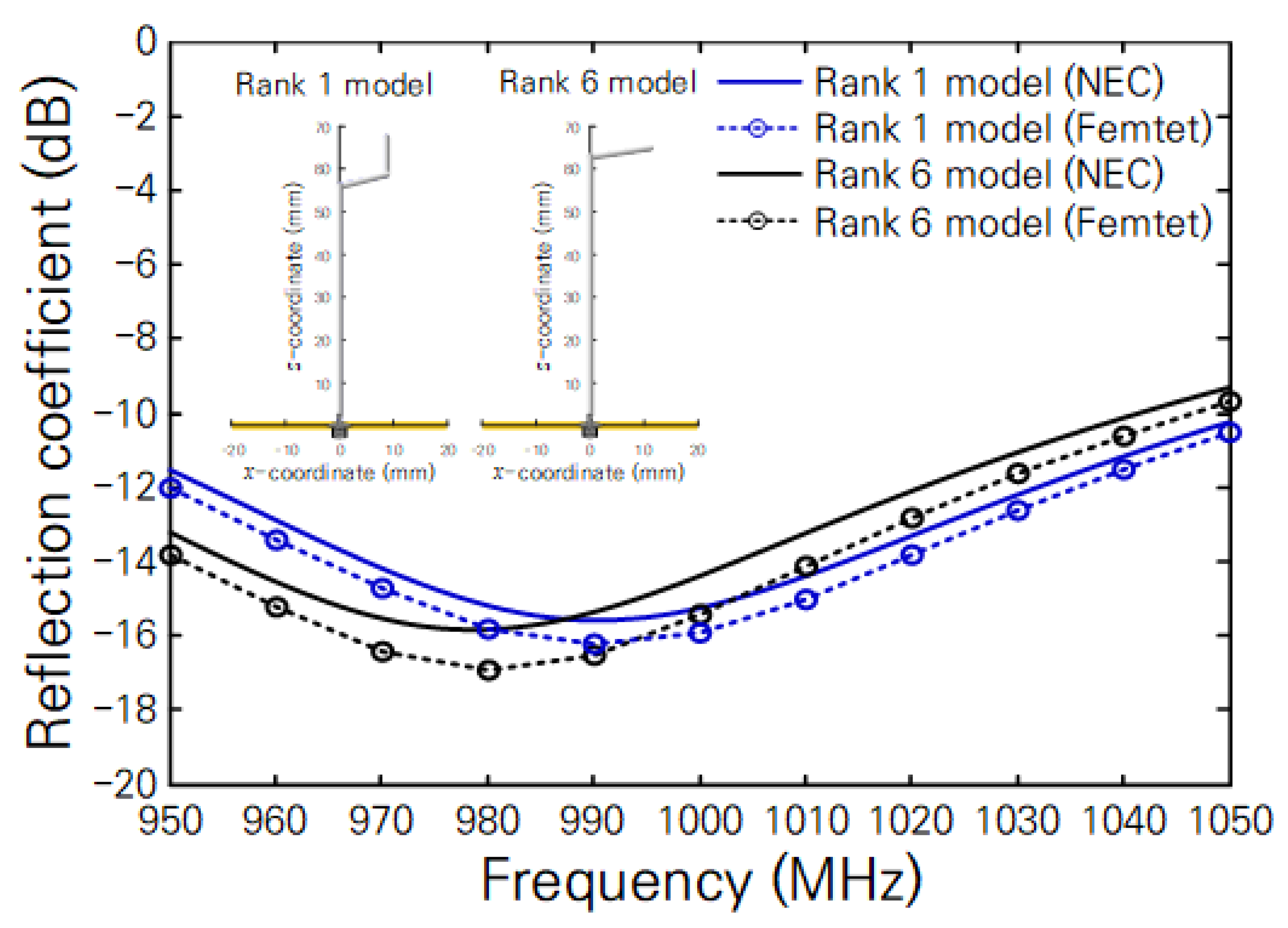
In
Table 6, the resulting antenna models can be divided into two types in geometry: one type is the monopole antenna with a top load such as the inverted-L antenna (the antennas with the ranks 6 and 9 in
Table 6) and the other type is the monopole antenna with a middle load (the antennas with the ranks 1~5, 7~8, and 10 in
Table 6). Thus, to further study two types of antennas, we examined the radiation pattern and the impedance matching characteristics of both types of antennas having the ranks 1 and 6 in
Table 6 using NEC and commercial EM simulators [
45]. From the simulated results, we confirmed that both antennas have a radiation pattern similar to that of an ideal monopole antenna. In addition, we represent the simulated reflection coefficients of both antennas as a function of frequency in
Figure 5, where the configuration of both antennas is illustrated in the insets. Although there is a small discrepancy in reflection coefficient owing to the applied analysis methods (NEC using the moment of method and Femtet using the finite element method), the result of
Figure 5 implies that both types of antennas operate well with small reflection coefficients in the interesting frequency range from 950 to 1050 MHz. This result also validates our ML model that can predict the impedance matching characteristic of the monopole antenna formed by a bent wire.
Based on the geometry depicted in the insets of
Figure 5, we represent the monopole antennas with top load and middle load in
Figure 6 as possible equivalent circuits [
46,
47,
48,
49,
50]. We expressed the vertical and horizontal wire sections as series and parallel RLC circuits, respectively. In addition, we assigned the parallel capacitance (
Ch2) caused by the open end of the antenna arm to the possible equivalent circuit. The series capacitance (
Cv) is negligible due to the current flowing along the vertical wire section. Thus, the parallel capacitances (
Ch1 and
Ch2) derived from the loads and the open end dominantly influence the impedance matching because it cancels out the series inductance (
Lv1) yielded by the vertical wire section. In the case of a monopole antenna with a middle load, we found that the basic operating principle is similar to that of a monopole antenna with a top load. Although the contribution of the second vertical wire section (third wire section) to the antenna impedance is small, we think it may finely control the induced current affecting antenna impedance.


