Abstract
Microseismic monitoring is an important technology used to evaluate hydraulic fracturing, and denoising is a crucial processing step. Analyses of the characteristics of acquired three-component microseismic data have indicated that the vertical component has a higher signal-to-noise ratio (SNR) than the two horizontal components. Therefore, we propose a new denoising method for three-component microseismic data using re-constrain variational mode decomposition (VMD). In this method, it is assumed that there is a linear relationship between the modes with the same center frequency among the VMD results of the three-component data. Then, the decomposition result of the vertical component is used as a constraint to the whole denoising effect of the three-component data. On the basis of VMD, we add a constraint condition to form the re-constrain VMD, and deduce the corresponding solution process. According to the synthesis data analysis, the proposed method can not only improve the SNR level of three-component records, it also improves the accuracy of polarization analysis. The proposed method also achieved a satisfactory effect for field data.
1. Introduction
Microseismic monitoring is a technology used to monitor the subsurface fracturing of rocks due to human activities [1,2,3,4]. This is the first step in recognizing microseismic event signals for microseismic monitoring. However, owing to the characteristics of microseismic event signals (e.g., low energy, high frequency, and short duration) they are easily disrupted by various factors, which increases the difficulty of the subsequent processing and interpretation. Therefore, it is necessary to denoise the monitoring record.
The denoising process for microseismic data is mainly divided into two basic strategies according to the type of data: multi-channel denoising and single-channel denoising [5]. For the multi-channel strategy, microseismic data are denoised by the spatial distribution information of the geophone. Gan et al. [6] used a median filter based on the seismic profile structure to suppress blending noise. Chao et al. [7] used a method based on the correlation between the three components of microseismic to identify the 3D shearlet transform coefficient and effectively remove the noise. Bai et al. [8] established a model based on the least squares method to decompose seismic data using the spatial and temporal relationships among multi-channel seismic data. The single-channel strategy is mainly used for denoising via time-frequency transformation and signal decomposition. Chakrabort et al. [9] used wavelet time-frequency analysis to suppress the seismic noise. Mousavi et al. [10] combined the synchrosqueezed continuous wavelet transform and a detection function to remove noise from the signal.
Noise reduction methods based on decomposition and reconstruction are widely used in single-channel noise reduction [11], such as empirical mode decomposition (EMD) [12,13] which is used to process the real and imaginary parts of the frequency domain of the signal in the time window to reduce random and coherent noise. Chen et al. [14] applied an AR mode to process the results of EMD in the frequency domain to reduce random noise. However, EMD has some drawbacks in practical applications, such as mode mixing [15]. Han et al. [16] used ensemble empirical mode decomposition (EEMD), which was proposed by Wu et al. [17] to overcome the problem of mode mixing and to process the real and imaginary parts of the frequency domain of the signal in the time window to reduce the noise. Chen et al. [18] applied wavelet threshold filtering to process the high-frequency intrinsic mode function (IMF) of the EEMD, and then reconstructed the high frequency and low frequency to reduce the noise. Dong et al. [19] combined the complex curvelet transform and complementary ensemble empirical mode decomposition (CEEMD) which was proposed by Yeh et al. [20] to improve the effect of decomposition. Zuo et al. [21] selected the IMFs of the CEEMD using the self-correlation coefficient, then used the wavelet packet threshold to process the IMFs, and finally reconstructed the IMFs to suppress the noise. Peng et al. [22] selected the EEMD mode by the variance contribution rates (VCRs), which removed the modes with VCR < 0.01 and others retained. Then, each retained mode was constructed as a Hankel matrix, and it was processed by principal component analysis (PCA) to complete denoising.
Compared with EMD, EEMD, and CEEMD, VMD can further decrease the redundant modes and solve the mode-mixing problem, and has a more powerful anti-noise performance [23]. Since then, many studies have applied VMD to reduce noise. Liu et al. [24] used VMD to perform time-frequency analysis of seismic data to suppress noise and highlight the geologic characteristics. Li et al. [25] selected IMFs to reconstruct a signal based on detrended fluctuation analysis (DFA). Huang et al. [26] performed a correlation analysis on the IMFs of the VMD to suppress the noise. Zhou et al. [27] combined VMD and odd spectrum analysis to remove the remaining low-frequency noise of the VMD. Li et al. [28] applied time-frequency peak filtering for the IMFs of VMD and reconstructed the signal to reduce noise. Liu et al. [29] used VMD to suppress ground rolling waves to achieve denoising. Zhang et al. [30] used the Akaike information criterion to judge the results of the VMD and selected the threshold to suppress the noise. In the above application research, most scholars have focused on processing IMFs to achieve a better denoising effect while using VMD. Li et al. [31] applied DFA to determine whether the VMD modes of the water inrush signals were random noise or a valid signal, and eliminated the noise in the mode using DFA.
Analyses of the characteristics of the acquired microseismic data found that the P-wave of the vertical component has a higher SNR than the horizontal components, which is not conducive to polarization analysis [32,33]. Therefore, a noise reduction method for the horizontal component is needed. When the three-component microseismic data are processed by VMD, the horizontal component is more easily affected by noise of similar frequency than the vertical component. This is because the level of random noise of the horizontal component is higher than that of the vertical component. Rodriguez et al. used a redundant dictionary to denoise the three components of microseismic data based on the sparse coefficient distribution of the three components [34]. Therefore, to improve the SNR of the horizontal component, it is assumed that each component consists of multiple IMFs, and there is a linear relationship between the modes of the same center frequency to limit the P-wave of the horizontal component by the vertical component. In this study, we propose a new method that adds a new constraint to the original formulas of VMD.
The proposed method simultaneously processes three-component microseismic data based on the VMD. However, the formulas for processing are different between the vertical component and the horizontal components. Based on the linear relationship among the three components of microseismic data, and the non-linear relationship of the random noise in the three-component data, the vertical component is processed by the original formula of VMD, and the horizontal components are processed by the re-constrained formula of VMD. The aim of this processing is to make the signal amplitude distribution of the horizontal components consistent with that of the vertical component as much as possible.
In the verification phase of the proposed method, a synthetic three-component data is designed in which the SNR horizontal component is relatively low, and that of the vertical component is relatively high. After denoising, the polarization characteristics of the data were analyzed to validate the effectiveness of the proposed method. In the practical phase, field microseismic data were processed based on the proposed method. The corresponding results show that the proposed method can effectively improve the SNR of three-component data as well as the precision of the polarization information.
2. Method
2.1. Variational Mode Decomposition
VMD is a signal decomposition method in which the IMF and corresponding center frequencies are obtained through iteration. The method first assumes that the original signal is decomposed into k mode components. It then takes the minimum Gaussian smoothness of each mode component as the goal. The sum of the modes is equal to the decomposed signal as the constraint for optimization. Finally, the decomposition results are obtained. The VMD expression is defined as follows:
where K is the number of decomposition modes, is the kth IMF, is the center frequency of the kth mode, is the original signal, is the sign of convolution, and is the Dirac delta function which indicates a unit impulse symbol.
The Lagrange multiplier method is used to solve the problem. The Lagrange multiplication operator is introduced to transform the constrained variational problem into an unconstrained variational problem. The updated formula is derived as follows:
where is the penalty factor, is the Fourier transform of the original signal, is the center frequency of the kth IMF of the horizontal component, is the Fourier transform of the kth IMF, and is the Fourier transform of the Lagrangian multipliers.
2.2. Re-Constraint of Variational Mode Decomposition
In the ideal state, the relationship between the three components of the microseismic data can be regarded as a linear relationship:
where and are horizontal components, is the vertical component, and and are coefficients that represent the linear relationships between the components.
Since the center frequencies of the P-wave and S-wave of the same microseismic event are different, this study assumed a linear relationship for the modes of the same (or close to) center frequencies in the VMD decomposition results of different components. Based on this relationship, we re-constrained the VMD and obtained a new formula that adds a new constraint condition:
where is the kth IMF after the decomposition of the vertical component, is the kth IMF after the decomposition of the horizontal component, and is a constant that expresses the linear relationship between the kth IMFs. The third line of Formula (4) is the re-constrained condition, indicating that there is a linear relationship between the modes.
By using the Lagrange multiplier method, we get the corresponding updated formulas:
where is the penalty factor, is the Fourier transform of the original signal, is the center frequency of the kth IMF of the horizontal component, and is the Fourier transform of the kth IMF. and are the Fourier transforms of the Lagrangian multipliers.
Under the noise-free condition, the VMD results for three-component data share the same frequency distributions. However, owing to the influence of various factors, the frequency distributions of the VMD results will be different in field data. Because the characteristic of the SNR of the vertical component is better than that of the horizontal component, we updated the horizontal component IMFs by using the center frequency of the vertical component IMFs in the iteration processing. The premise of using this method to process three-component microseismic data is that the SNR of the vertical component is higher than that of the horizontal components. Thus, we obtained the new updated formulas:
where is the penalty factor, is the Fourier transform of the original signal, is the center frequency of the kth IMF of the vertical component, and is the Fourier transform of the kth IMF. and are the Fourier transforms of the Lagrangian multipliers.
As shown in Figure 1, the processing flow of the re-constrain VMD is as follows:
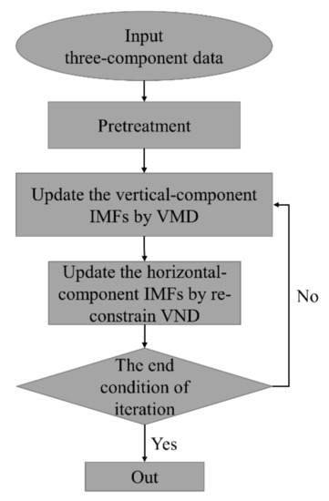
Figure 1.
Flow chart of processing the three-component microseismic data by re-constrain VMD.
- Load the initial three-component microseismic data.
- Expend the data using a mirror image against the boundary effect, and perform the Fourier transform for the original data. The related parameters of the subsequent processing are initialized.
- Update the vertical component variable using VMD updated formulas as Formula (2).
- Update the parameters of the horizontal components using updated re-constrain VMD formula as in Formula (6).
- Judge whether the end condition of iteration is satisfied. The end condition is determined by the maximum number of iterations. If the condition is not satisfied, repeat Step 3.
- Perform the inverse Fourier transform for the previous output, and remove the mirror data. Then, the final result is obtained.
3. Synthetic Data
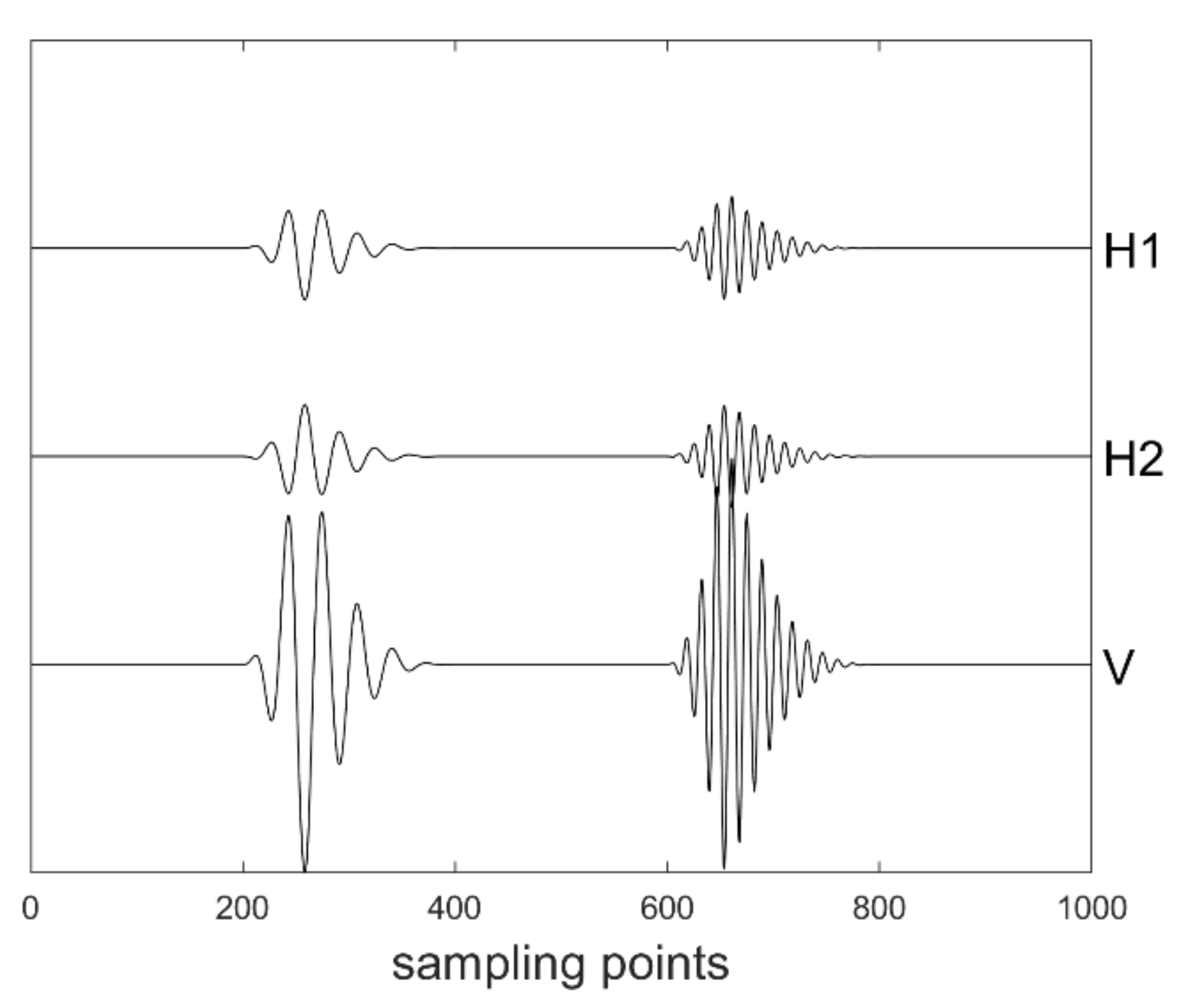
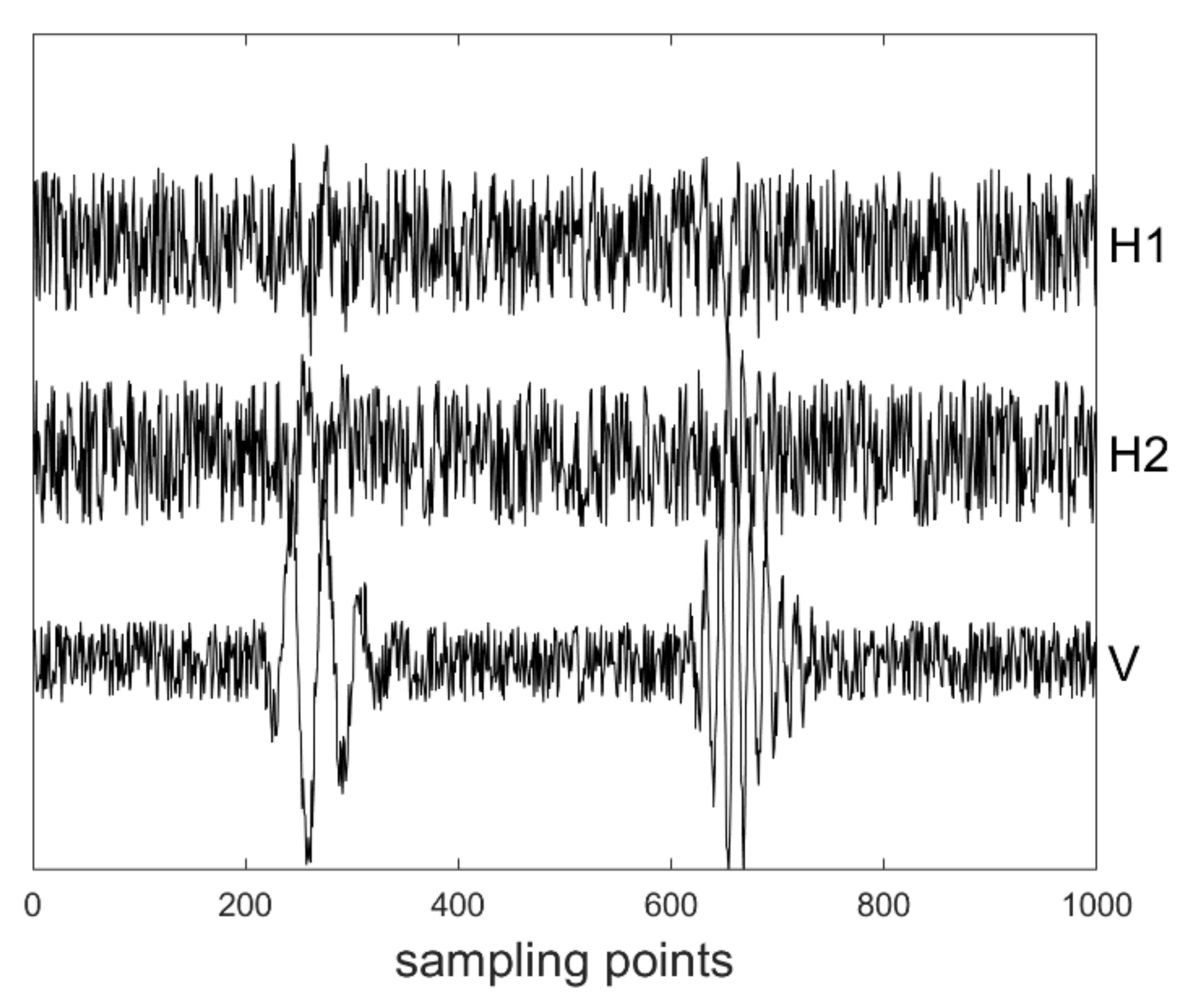
We used an attenuated simple harmonic to verify the effectiveness of this method. Figure 2 shows pure attenuated harmonic three-component data with frequencies of 30 Hz and 70 Hz. Figure 3 shows waves contaminated with random noise. The SNR of the horizontal component is set to −10 dB, and the SNR of the vertical component is set to 5 dB. In this study, we used the SNR, which is defined as:
where is the pure synthetic signal, is random noise, and is the number of sampling points.

Figure 2.
The pure synthetic three-component signal. H1 and H2 denote two horizontal components, V denotes the vertical component.
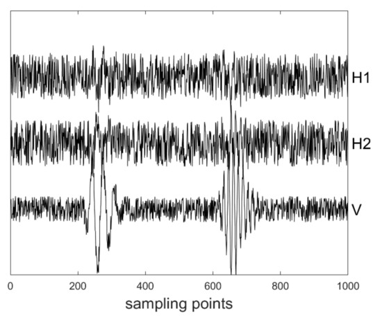
Figure 3.
The synthetic data contaminated with random noise.
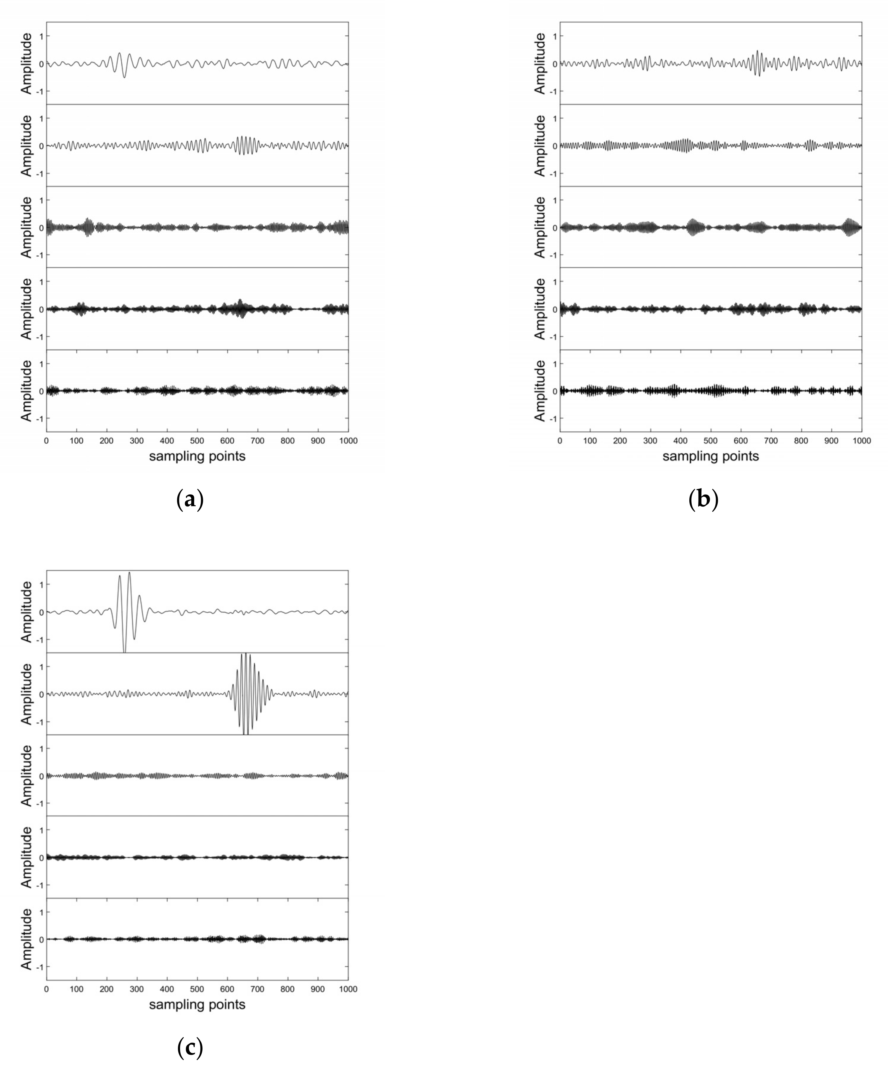
Figure 4 shows the VMD results of three-component data. Since the parameter k of VMD only impacts the frequency representation performance, it has no noticeable impact on the reconstruction performance [24]. In addition, the proposed method only focuses on the frequency representation of the vertical component, which is viewed as a re-constraint condition. Therefore, the parameter k for each component was set to the same value in this study.

Figure 4.
The IMFs of VMD for the synthetic three-component data. (a) The VMD result of the H1 component. (b) The VMD result of the H2 component. (c) The VMD result of the vertical component.
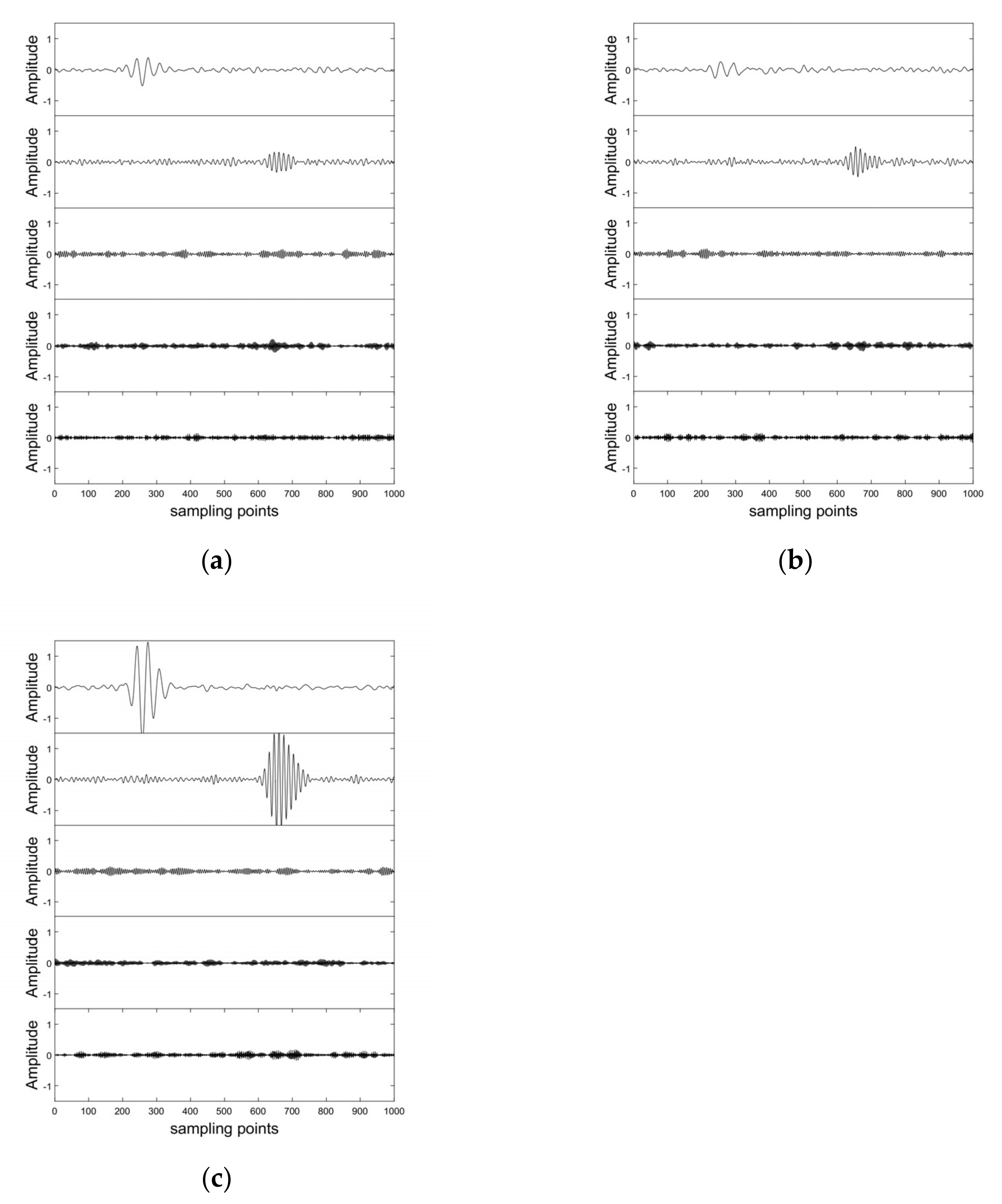
Figure 5 shows the decomposition results of the three-component synthetic data obtained by the re-constrain VMD. As shown in Figure 5, the redundant amplitude of the nonlinear relationship information was removed. The remaining modes were also suppressed because they are all random signals and have no direct correlation.
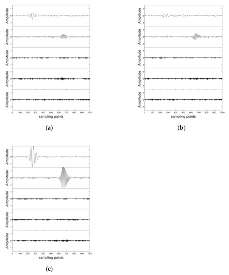
Figure 5.
The IMFs of re-constrain VMD for the synthetic three-component data. (a) The re-constrain VMD result of the H1 component. (b) The re-constrain VMD result of the H2 component. (c) The re-constrain VMD result of the vertical component.
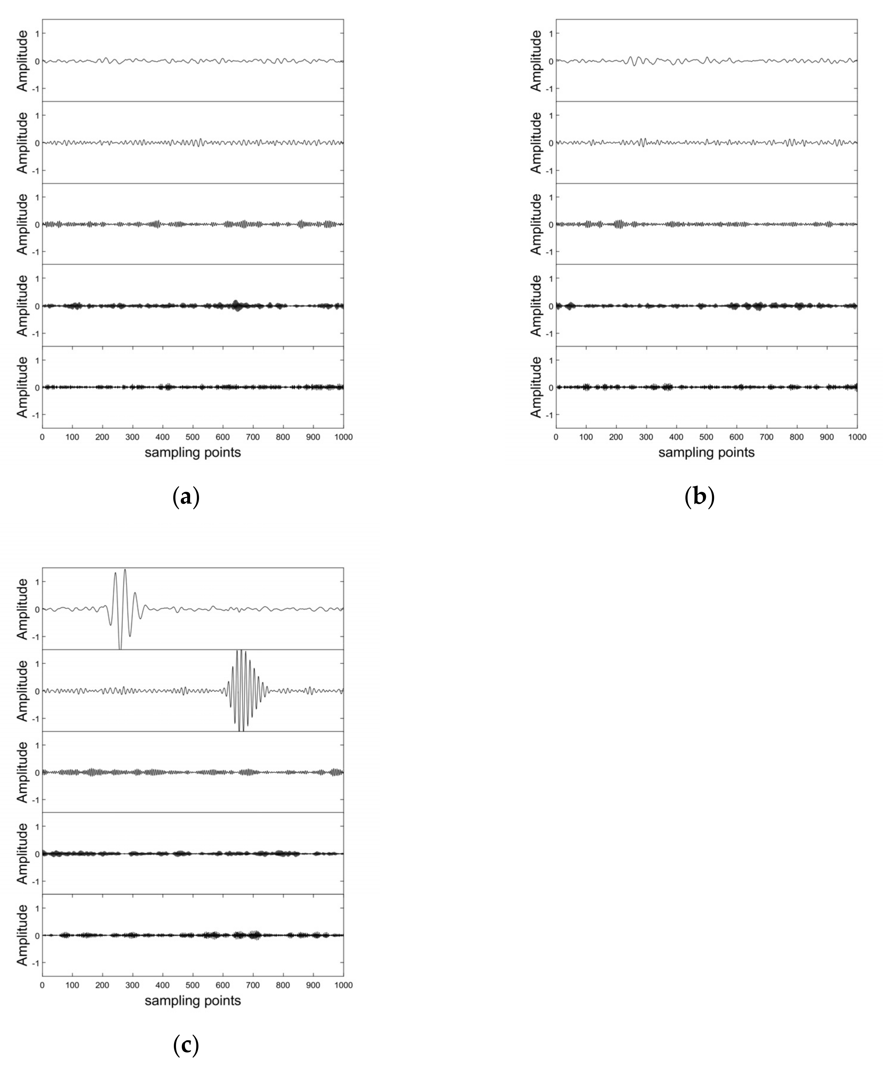
To prevent the re-constrained modes of two horizontal components (of which the SNR is low) from being an illusion of noise fitting (in other words, noise is regarded as an effective component of the signal to participate in the reconstruction processing), we removed the pure synthetic signal and performed the re-constrain VMD for these two components. Figure 6 shows the corresponding results. For the re-constrained modes in the two horizontal components, there was a weak correlation with the vertical component after re-constrained decomposition, indicating that the re-constrained modes of the two horizontal components were also affected by random noise, and the degree of influence was quite limited.
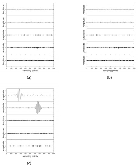
Figure 6.
The IMFs of re-constrain VMD for the three-component data and the horizontal components without pure synthetic data. (a) The re-constrain VMD result of the H1 component without valid data. (b) The re-constrain VMD result of the H2 component without valid data. (c) The re-constrain VMD result of the vertical component with valid data.
The first and second modes were reconstructed as a result of simple noise reduction. In Figure 7, it can be seen that compared with the VMD results, the results of re-constrain VMD could obtain better polarization characteristics and remove more background noise.
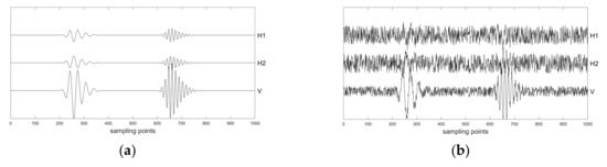
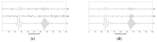
Figure 7.
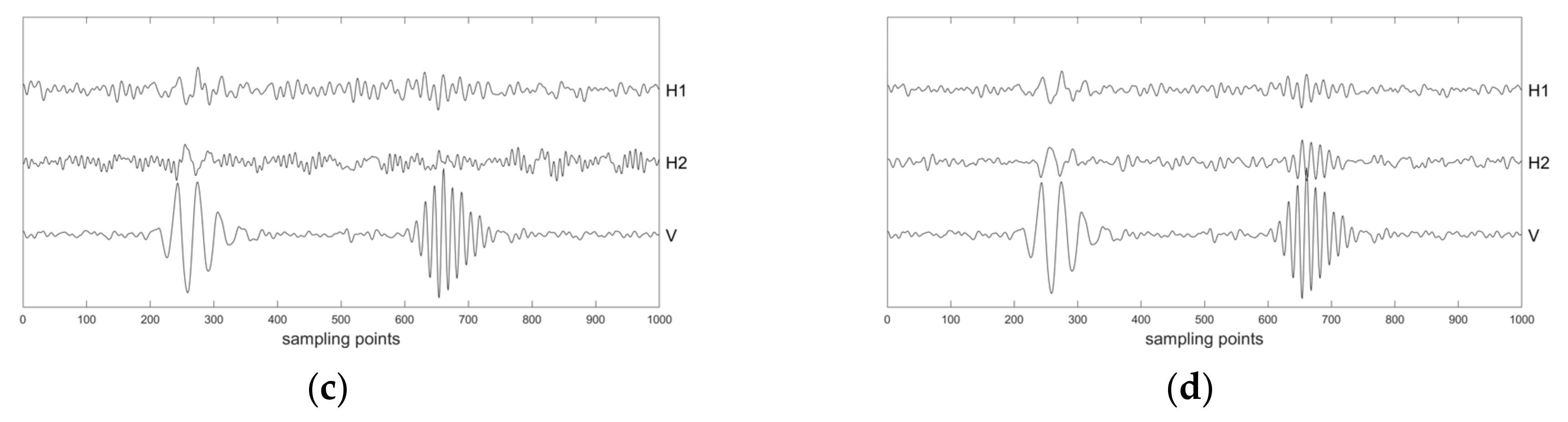
Denoising results of the synthetic microseismic data. (a) The synthetic data without noise. (b) The synthetic data with noise. (c) The denoising result of VMD. (d) The denoising result of re-constrain VMD.
To better evaluate its denoising effect, we analyzed the polarization characteristics of the 30 Hz signal in the three-component data. The length of the selected time window was an entire period, and the 230th sampling point was manually selected as the starting point of this window, as shown in Figure 8.
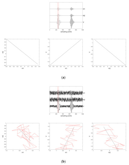
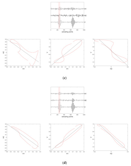
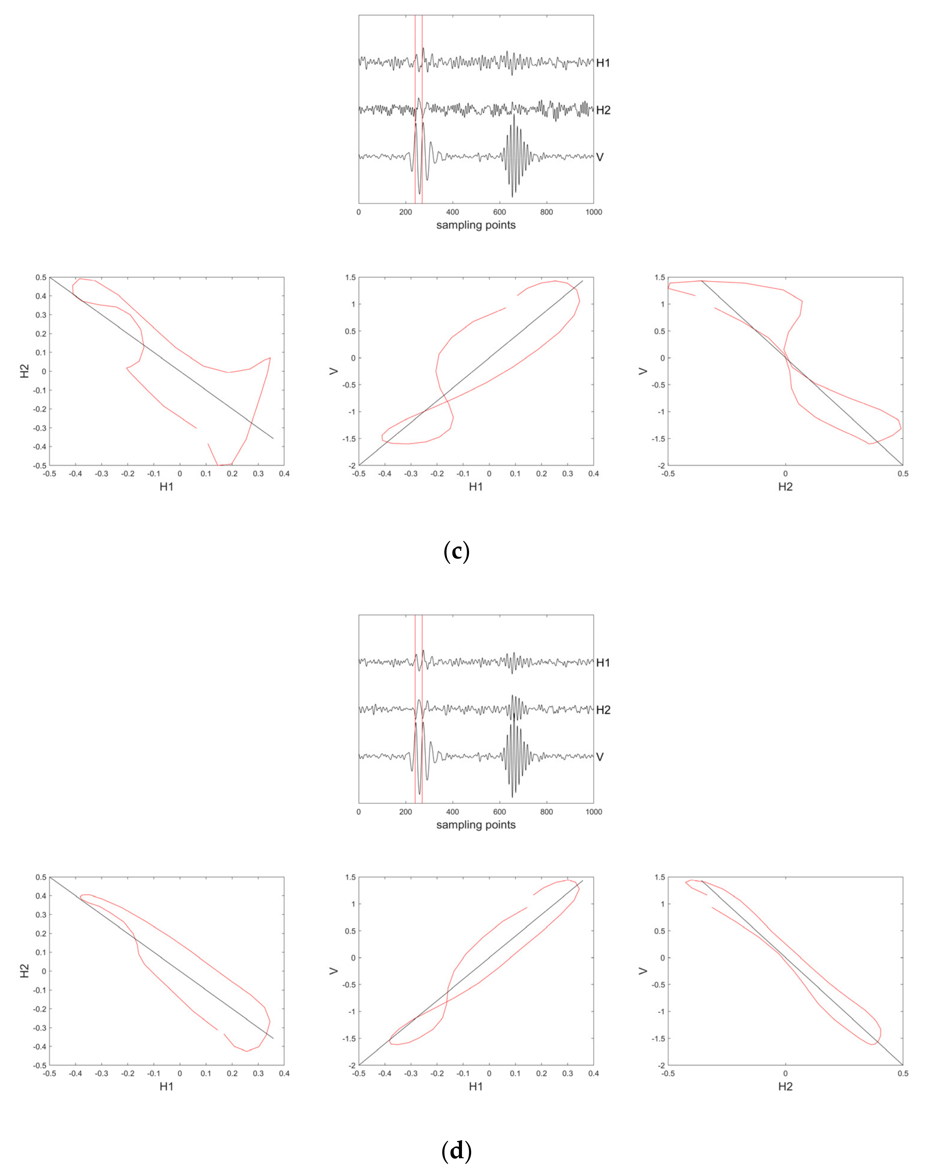
Figure 8.
Comparison of hodogram analysis of the synthetic data. (a) The synthetic data without noise (the two red lines are the time window of the hodograms) and the hodograms of the three-component data. (b) The synthetic data with noise (the two red lines are the time window of the hodograms) and the hodograms of the three-component data (the black lines are hodograms of (a)). (c) The denoising result obtained by using VMD (the two red lines are the time window of the hodograms) and the hodograms of the three-component data (the black lines are hodograms of (a)). (d) The denoising result obtained using re-constrain VMD (the two red lines are the time window of the hodograms) and the hodograms of three-component data (the black lines are the hodograms of (a)).
In the synthetic data in Figure 8, the two red lines indicate the range of the selected windows for polar analysis. It is evident that the polarization directions were changed for the synthetic data contaminated with random noise. After denoising based on VMD and re-constrain VMD, the accuracy of the calculated polarization directions was greatly improved. In addition, the results of hodograms based on re-constrain VMD were more compact than those based on VMD.
4. Field Microseismic Data
The field three-component microseismic event data were acquired in the hydraulic fracturing of a shale gas reservoir. The original waveforms of this microseismic event are shown in the first row of Figure 9. These microseismic data include the P-wave and S-wave of the microseismic event. The range of the P-wave is approximately from the 1000th sampling point to the 1450th sampling point, and the range of S-wave is approximately from the 1450th sampling point to the 2000th sampling point. Because of the formation mechanism of microseismic events, there is a partial overlap between the P-wave and S-wave. The SNR of the vertical component is better than that of the two horizontal components. The noise reduction results obtained using VMD and re-constrain VMD are shown. Comparing the waveforms between the original data and denoising results, the random noise was effectively suppressed by both methods.
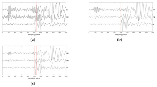
Figure 9.
Comparison of denoising results between VMD and re-constrain VMD. (a) The original waveforms of a three-component microseismic event. (b) The denoising result obtained using VMD. (c) The denoising result obtained using re-constrain VMD.
As shown in Figure 9, these two methods could suppress random noise to a certain extent. According to the original waveform of the horizontal component H1, the SNR of the P-wave is relatively low. Comparing the H1 components of the two groups’ denoising results, it can be seen that the P-wave waveforms of microseismic data were not well recovered using VMD. Correspondingly, the waveforms of the P-wave were more obvious after using re-constrain VMD. It can also be seen that the background noise was better suppressed after using re-constrain VMD, but this effect was controlled by the background noise intensity of the vertical component.
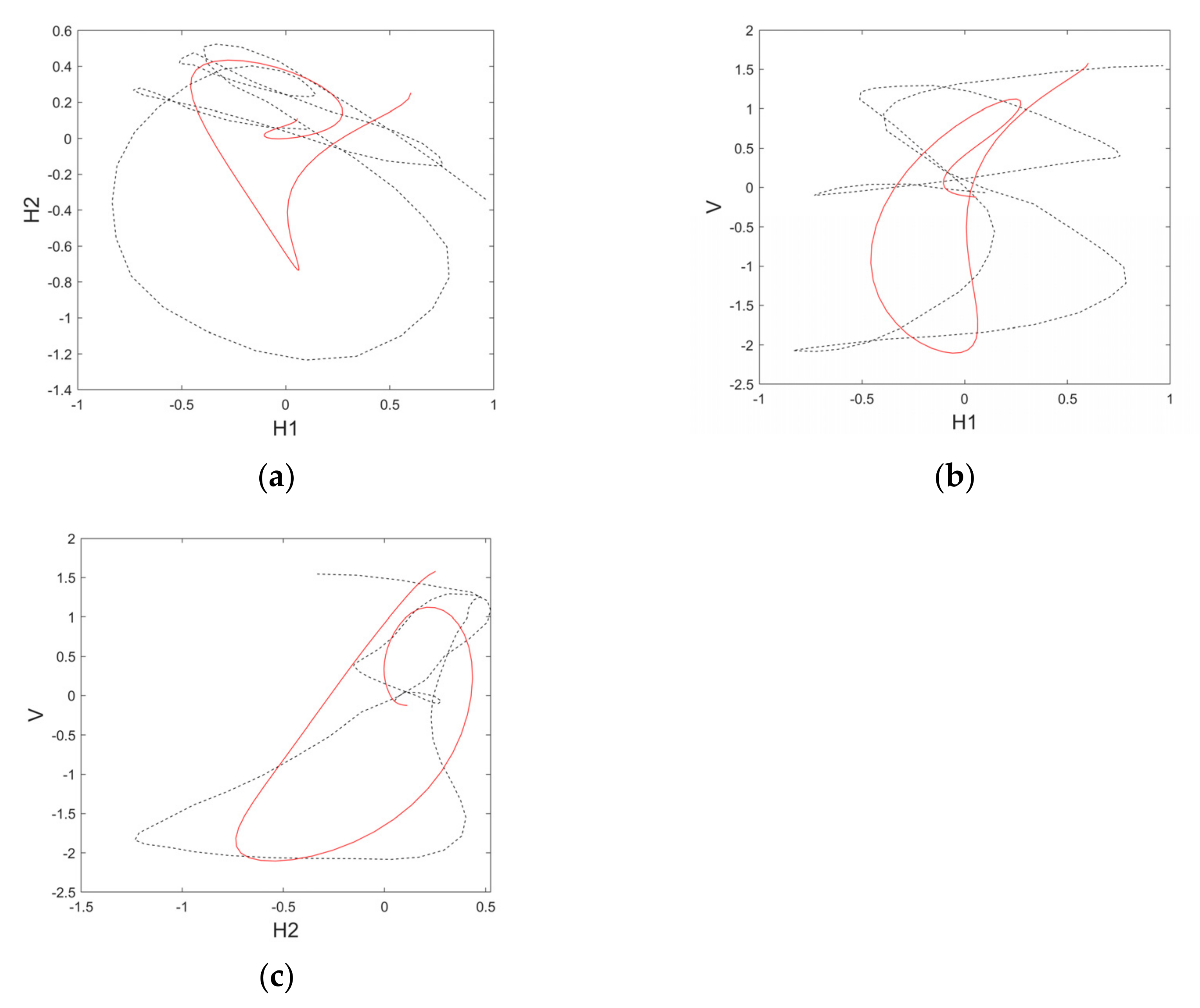
Because the P-wave is commonly used to analyze the polarization direction of microseismic events, we selected from the 1000th point to the 1070th point as the time window range, which is indicated by the red lines in Figure 9. The data in the time window were used to analyze the polarization and to judge the denoising effect. After denoising using VMD and re-constrain VMD, the polarization characteristics of the denoising results are shown in Figure 10 and Figure 11.
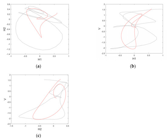
Figure 10.
The hodograms of microseismic event data after denoising using VMD. The black dotted lines represent the polarization characterization before denoising, and the red solid lines represent the polarization characterization after denoising. (a) The horizontal component H1 vs. horizontal component H2 hodogram. (b) The horizontal component H1 vs. vertical component V hodogram. (c) The horizontal component H2 vs. vertical component V hodogram.
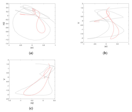
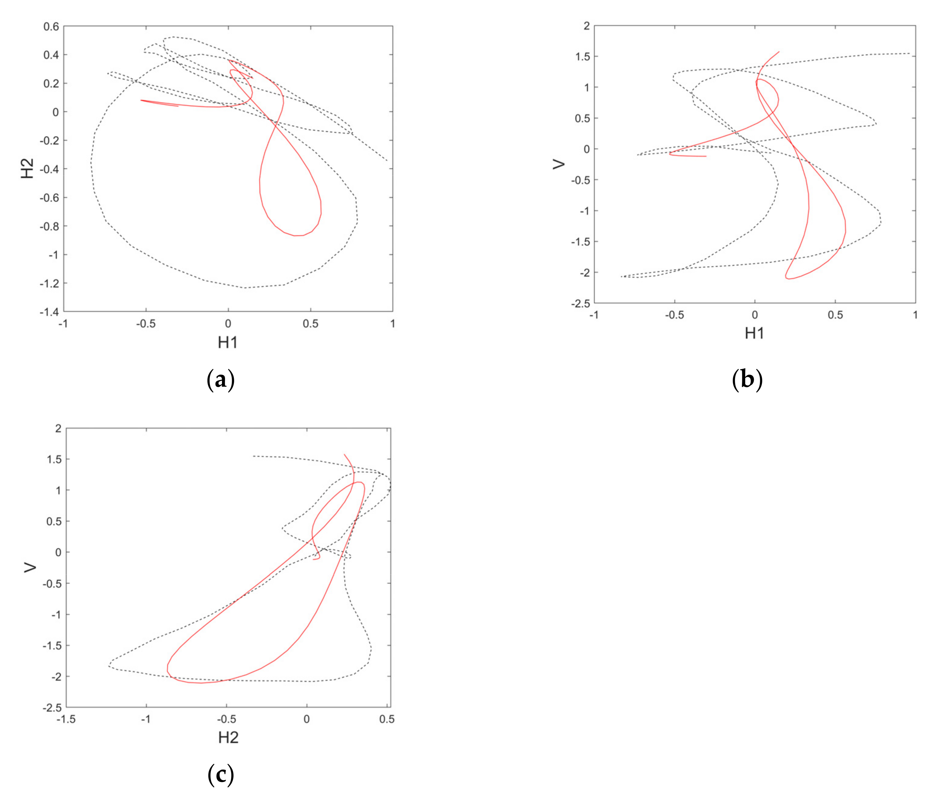
Figure 11.
The hodograms of microseismic event data after denoising using re-constrain VMD. The black dotted lines represent the polarization characterization before denoising, and the red solid lines represent the polarization characterization after denoising. (a) The horizontal component H1 vs. horizontal component H2 hodogram. (b) The horizontal component H1 vs. vertical component V hodogram. (c) The horizontal component H2 vs. vertical component V hodogram.
In this study, the enhancement of polarization information by denoising was evaluated by determining whether the polarization characteristic of the curve of the hodogram was clear, compact, and self-consistent. It was largely straightforward to determine whether the polarization characteristic of the curve was clear, except for the H1–H2 hodogram in Figure 10. Regarding compactness, all hodograms in Figure 11 are better than those in Figure 10. Regarding self-consistency, according to the positive or negative correlation among the three components, the hodograms in Figure 11 are better than those in Figure 10.
5. Conclusions
The proposed method mainly focuses on solving the challenge of low-SNR horizontal components of microseismic data. Among the different components, there is no correlation for random noise, and there is a linear relationship for the signal. For most field three-component microseismic data, the SNR of the vertical component is better than that of the two horizontal components. Therefore, by adding a new constraint to the VMD and modifying the new updated formulas, we propose the re-constrain VMD. The new constraint is used to represent the characteristics of linear relationships for signal and random noise among the three components of the data.
According to the denoising results for the synthetic data and field microseismic data, we found that the proposed method could suppress random noise to a certain extent, and the effect was better than that of VMD. The subsequent polarization analysis also showed that the proposed method could obtain better polarization characteristics.
Author Contributions
Each author contributed to the present paper. P.W. conceived the method and directed the experiments; Z.C. and Q.M. performed the experiments; Z.C. analyzed the data and wrote the article; Z.G. supervised the experiments and the article. All authors have read and agreed to the published version of the manuscript.
Funding
This research was funded by the state key program of National Natural Science Foundation of China, grant No. 42030805 and the Open Fund of Key Laboratory of Exploration Technologies for Oil and Gas Resources (Yangtze University), Ministry of Education, grant No. K2021-19.
Institutional Review Board Statement
Not applicable.
Informed Consent Statement
Not applicable.
Data Availability Statement
Not applicable.
Acknowledgments
Not applicable.
Conflicts of Interest
The authors declare no conflict of interest.
References
- Dyer, B.C.; Schanz, U.; Ladner, F.; Häring, M.O.; Spillman, T. Microseismic imaging of a geothermal reservoir stimulation. Lead. Edge 2008, 27, 856–869. [Google Scholar] [CrossRef]
- Lellouch, A.; Lindsey, N.J.; Ellsworth, W.L.; Biondi, B.L. Comparison between Distributed Acoustic Sensing and Geophones: Downhole Microseismic Monitoring of the FORGE Geothermal Experiment. Seism. Res. Lett. 2020, 91, 3256–3268. [Google Scholar] [CrossRef]
- Liu, X.; Liu, Q.; Liu, B.; Kang, Y. A Modified Bursting Energy Index for Evaluating Coal Burst Proneness and Its Application in Ordos Coalfield, China. Energies 2020, 13, 1729. [Google Scholar] [CrossRef] [Green Version]
- Dwan, F.; Qiu, J.; Zhou, M.; Yuan, R.; Zhang, Z.; Jin, L.; Wang, S.; Li, X.; Lin, M.; Liang, B.; et al. Sichuan Shale Gas Microseismic Monitoring: Acquisition, Processing, and Integrated Analyses. In Proceedings of the International Petroleum Technology Conference, Beijing, China, 26–28 March 2013. [Google Scholar] [CrossRef]
- Wang, H.; Zhang, Q.; Zhang, G.; Fang, J.; Chen, Y. Self-training and learning the waveform features of microseismic data using an adaptive dictionary. Geophysics 2020, 85, KS51–KS61. [Google Scholar] [CrossRef]
- Gan, S.; Wang, S.; Chen, Y.; Chen, X.; Xiang, K. Separation of simultaneous sources using a structural-oriented median filter in the flattened dimension. Comput. Geosci. 2016, 86, 46–54. [Google Scholar] [CrossRef]
- Zhang, C.; Van Der Baan, M. Multicomponent microseismic data denoising by 3D shearlet transform. Geophysics 2018, 83, A45–A51. [Google Scholar] [CrossRef]
- Bai, M.; Chen, W.; Chen, Y. Nonstationary Least-Squares Decomposition With Structural Constraint for Denoising Multi-Channel Seismic Data. IEEE Trans. Geosci. Remote Sens. 2019, 57, 10437–10446. [Google Scholar] [CrossRef]
- Chakraborty, A.; Okaya, D. Frequency-time decomposition of seismic data using wavelet-based methods. Geophysics 1995, 60, 1906–1916. [Google Scholar] [CrossRef] [Green Version]
- Mousavi, S.M.; Langston, C.; Horton, S.P. Automatic microseismic denoising and onset detection using the synchrosqueezed continuous wavelet transform. Geophysics 2016, 81, V341–V355. [Google Scholar] [CrossRef]
- Lv, H. Single-channel and multi-channel seismic random noise suppression based on the regularized non-stationary decomposition. J. Appl. Geophys. 2020, 175, 103986. [Google Scholar] [CrossRef]
- Huang, N.E.; Shen, Z.; Long, S.R.; Wu, M.C.; Shih, H.H.; Zheng, Q.; Yen, N.-C.; Tung, C.C.; Liu, H.H. The empirical mode decomposition and the Hilbert spectrum for nonlinear and non-stationary time series analysis. Proc. R. Soc. London. Ser. A Math. Phys. Eng. Sci. 1998, 454, 903–995. [Google Scholar] [CrossRef]
- Bekara, M.; Van Der Baan, M. Random and coherent noise attenuation by empirical mode decomposition. Geophysics 2009, 74, V89–V98. [Google Scholar] [CrossRef]
- Chen, Y.; Ma, J. Random noise attenuation by f-x empirical-mode decomposition predictive filtering. Geophysics 2014, 79, V81–V91. [Google Scholar] [CrossRef]
- Mandic, D.P.; Rehman, N.U.; Wu, Z.; Huang, N.E. Empirical Mode Decomposition-Based Time-Frequency Analysis of Multivariate Signals: The Power of Adaptive Data Analysis. IEEE Signal Process. Mag. 2013, 30, 74–86. [Google Scholar] [CrossRef]
- Han, J.; van der Baan, M. Microseismic and seismic denoising via ensemble empirical mode decomposition and adaptive thresholding. Geophysics 2015, 80, KS69–KS80. [Google Scholar] [CrossRef] [Green Version]
- Wu, Z.; Huang, N.E. Ensemble empirical mode decomposition: A noise-assisted data analysis method. Adv. Adapt. Data Anal. 2009, 1, 1–41. [Google Scholar] [CrossRef]
- Chen, W.; Zhang, D.; Chen, Y. Random noise reduction using a hybrid method based on ensemble empirical mode decomposition. J. Seism. Explor. 2017, 26, 227–249. [Google Scholar]
- Dong, L.; Wang, D.; Zhang, Y.; Zhou, D. Signal enhancement based on complex curvelet transform and complementary ensemble empirical mode decomposition. J. Appl. Geophys. 2017, 144, 144–150. [Google Scholar] [CrossRef]
- Yeh, J.-R.; Shieh, J.-S.; Huang, N.E. Complementary ensemble empirical mode decomposition: A novel noise enhanced data analysis method. Adv. Adapt. Data Anal. 2010, 2, 135–156. [Google Scholar] [CrossRef]
- Zuo, L.-Q.; Sun, H.-M.; Mao, Q.-C.; Liu, X.-Y.; Jia, R.-S. Noise Suppression Method of Microseismic Signal Based on Complementary Ensemble Empirical Mode Decomposition and Wavelet Packet Threshold. IEEE Access 2019, 7, 176504–176513. [Google Scholar] [CrossRef]
- Peng, K.; Guo, H.; Shang, X. EEMD and Multiscale PCA-Based Signal Denoising Method and Its Application to Seismic P-Phase Arrival Picking. Sensors 2021, 21, 5271. [Google Scholar] [CrossRef] [PubMed]
- Dragomiretskiy, K.; Zosso, D. Variational Mode Decomposition. IEEE Trans. Signal Process. 2013, 62, 531–544. [Google Scholar] [CrossRef]
- Liu, W.; Cao, S.; Chen, Y. Applications of variational mode decomposition in seismic time-frequency analysis. Geophysics 2016, 81, V365–V378. [Google Scholar] [CrossRef]
- Li, F.; Zhang, B.; Verma, S.; Marfurt, K.J. Seismic signal denoising using thresholded variational mode decomposition. Explor. Geophys. 2018, 49, 450–461. [Google Scholar] [CrossRef]
- Huang, Y.; Bao, H.; Qi, X. Seismic Random Noise Attenuation Method Based on Variational Mode Decomposition and Correlation Coefficients. Electronics 2018, 7, 280. [Google Scholar] [CrossRef] [Green Version]
- Zhou, Y.; Zhu, Z. A hybrid method for noise suppression using variational mode decomposition and singular spectrum analysis. J. Appl. Geophys. 2019, 161, 105–115. [Google Scholar] [CrossRef]
- Li, Z.; Gao, J.; Liu, N.; Sun, F.; Jiang, X. Random noise suppression of seismic data by time–frequency peak filtering with variational mode decomposition. Explor. Geophys. 2019, 50, 634–644. [Google Scholar] [CrossRef]
- Liu, W.; Duan, Z. Seismic Signal Denoising Using f-x Variational Mode Decomposition. IEEE Geosci. Remote Sens. Lett. 2019, 17, 1313–1317. [Google Scholar] [CrossRef]
- Zhang, J.; Dong, L.; Xu, N. Noise Suppression of Microseismic Signals via Adaptive Variational Mode Decomposition and Akaike Information Criterion. Appl. Sci. 2020, 10, 3790. [Google Scholar] [CrossRef]
- Li, L.; Jin, H.; Chen, Y.; Cheng, S.; Hu, H.; Wang, S. Noise reduction method of microseismic signal of water inrush in tunnel based on variational mode method. Bull. Eng. Geol. Environ. 2021, 2021, 6497–6512. [Google Scholar] [CrossRef]
- Mukuhira, Y.; Poliannikov, O.V.; Fehler, M.C.; Moriya, H. Low-SNR Microseismic Detection Using Direct P-Wave Arrival Polarization. Bull. Seism. Soc. Am. 2020, 110, 3115–3129. [Google Scholar] [CrossRef]
- Chen, Z. A multi-window algorithm for automatic picking of microseismic events on 3-C data. In Proceedings of the 2005 SEG Annual Meeting, Houston, TX, USA, 6–11 November 2005. [Google Scholar] [CrossRef]
- Vera Rodriguez, I.; Bonar, D.; Sacchi, M. Microseismic data denoising using a 3C group sparsity constrained time-frequency transform. Geophysics 2012, 77, V21–V29. [Google Scholar] [CrossRef]


Publisher’s Note: MDPI stays neutral with regard to jurisdictional claims in published maps and institutional affiliations. |
© 2021 by the authors. Licensee MDPI, Basel, Switzerland. This article is an open access article distributed under the terms and conditions of the Creative Commons Attribution (CC BY) license (https://creativecommons.org/licenses/by/4.0/).