Laboratory Measurements of Zeta Potential in Fractured Lewisian Gneiss: Implications for the Characterization of Flow in Fractured Crystalline Bedrock

Abstract

Despite the broad range of interest and possible applications, the controls on the electric surface charge and the zeta potential of gneiss at conditions relevant to naturally fractured systems remain unreported. There are no published zeta potential measurements conducted in such systems at equilibrium, hence, the effects of composition, concentration and pressure remain unknown. This study reports zeta potential values for the first time measured in a fractured Lewisian gneiss sample saturated with NaCl solutions of various concentrations, artificial seawater and artificial groundwater solutions under equilibrium conditions at confining pressures of 4 MPa and 7 MPa. The constituent minerals of the sample were identified using X-ray diffraction and linked to the concentration and composition dependence of the zeta potential. The results reported in this study demonstrate that the zeta potential remained negative for all tested solutions and concentrations. However, the values of the zeta potential of our Lewisian gneiss sample were found to be unique and dissimilar to pure minerals such as quartz, calcite, mica or feldspar. Moreover, the measured zeta potentials were smaller in magnitude in the experiments with artificial complex solutions compared with those measured with NaCl, thus suggesting that divalent ions (Ca²⁺, Mg²⁺ and SO₄²⁻) acted as potential determining ions. The zeta potential was also found to be independent of salinity in the NaCl experiments, which is unusual for most reported data. We also investigated the impact of fracture aperture on the electrokinetic response and found that surface electrical conductivity remained negligibly small across the range of the tested confining pressures. Our novel results are an essential first step for interpreting field self-potential (SP) signals and facilitate a way forward for characterization of water flow through fractured basement aquifers.

1. Introduction

Fractured crystalline basement aquifers are predominantly made of granites and gneisses are widespread [1] and are locally important for rural water supplies and as a geothermal resource (e.g., [2,3]). They are predominantly made of granites and gneisses and mostly occur in Precambrian shield regions covering large parts of Europe (especially Scandinavia), North and South America, Africa, India, Australia, and in Precambrian orogens such as the Lewisian basement of NW Scotland [3].

Unlike in tropical regions, where deep weathering of crystalline basement rocks produce a porous aquifer (saprolite) with relatively high water storage capacity [4], in temperate/cold regions where weathering has been limited or absent, or scraped by glacier erosion, groundwater flow is mostly restricted to connected fracture networks and, while fracture porosity is generally low, permeability can be relatively high (e.g., [5,6]).

Understanding the fluid flow and storage properties in fractured rocks is challenging due to the discrete nature, heterogeneity and scale effect of fracture systems (e.g., [7,8,9]). It is of major importance to understand fractured systems in terms of hydraulically active fractures (versus hydraulically inactive) controlled by fracture connectivity, and fracture geometry including aperture and direction, which overall results in strong anisotropy in groundwater flow.

Direct characterization of groundwater flow patterns in fractured rock aquifers usually involves borehole studies including hydraulic testing or tracer testing methods, or a combination of both (e.g., [10,11]). Due to low permeability and storativity of fractured aquifers, both methods usually provide information on aquifer and fracture network properties only in the close vicinity of the borehole [12]. It is challenging to extrapolate the information to site- or region-scale due to large, multiscale heterogeneities of fracture systems (e.g., [7,13,14]). Surface geophysical methods are increasingly used to support interpolation to larger scales by providing indirect quantitative information on the heterogeneities of fracture networks and associated equivalent hydrodynamic properties (e.g., [12,15]). Most common geophysical methods used for this purpose are electrical resistivity tomography (ERT, e.g., [16]), ground-penetrating radar (GPR, e.g., [17]), magnetic resonance [18], or a combination of these techniques.

However, these methods are usually applied to provide equivalent isotropic flow/storage properties of the bulk aquifer over a certain volume, or structural information, rather than the flow properties of the fracture networks themselves. They are also expensive to deploy in the field in terms of effort and equipment. More recently, alternative, low-cost surface geophysical methods, such as self-potential (SP), have shown promise to better quantify fracture flow, including anisotropy, in crystalline rock aquifers (e.g., [19,20,21]).

SP arises in response to pressure concentration or temperature gradients associated with the motion of water or aqueous solutions [22]; therefore, any signal acquired from electrode arrays reflects the dynamic behavior of the effective aquifer pore space, i.e., hydraulically active fractures in fractured rock aquifers. The method is passive and can be applied using surface arrays installed into the overlying soil layer (e.g., [23]) or discrete observation boreholes equipped with electrodes (e.g., [24]) and, therefore, provide information at both high spatial and temporal resolution.

A numerical study [25] investigated the potential application of SP to characterize fractured systems, and the authors demonstrated that the simulated SP signal not only accurately predicted preferential orientation of hydraulically active fractures but also identified fracture-matrix fluid exchange. The reported results indicated that the SP signal was primarily sensitive to hydraulically active fractures having matrix-fracture fluid exchange, thus implying that a non-zero porosity and near-zero permeability should be assigned to the matrix, which accommodated a significant volume of water but did not contribute significantly to the flow, and would be required to characterize the flow using SP. Assuming a strictly impervious matrix (zero porosity and zero permeability), resulted in a negligibly small electrokinetic signal. However, the authors assumed their fracture apertures to range between 0.2 mm and 2 mm, thus implying near-zero pressure gradients along the fractures and, therefore, a negligible SP response. In real fractured crystalline rocks, the aperture is expected to be a few orders of magnitude smaller (as discussed below); hence, the SP signal in such systems would be measurable even without matrix-fracture fluid exchange, thus, making the SP method applicable for such systems. In support of our hypothesis, a field SP survey on a crystalline bedrock [20] clearly demonstrated that azimuthal SP gradients tightly correlated with the investigated fracture strike orientation even though the matrix of the studied field site was impermeable and non-porous, consistent with the nature of crystalline bedrocks. Moreover, azimuthal resistivity surveys conducted on the same site showed the expected orientation of high water content, but were completely misaligned with the measured fracture network, thus making the SP method superior for identifying hydraulically active fractures, essential for accurate characterization of groundwater storage and flow.

Other published studies used the SP method to characterize and predict temporal variation of head gradients in a fractured aquifer as the results of diurnal tide cycles [26], and also to characterize saltwater intrusion into freshwater chalk aquifers (e.g., [24,27]). These studies demonstrated that the flow of freshwater and/or seawater through fractures was responsible for observed temporal and spatial variation of the SP measured in an observation borehole, even though the matrix was nearly impermeable. Moreover, the observed SP precursor that preceded seawater breakthrough was demonstrated to result from spatial variability of the so-called exclusion efficiency that was primarily associated with existing anisotropy in mineralogy and permeability of the aquifer. Therefore, not only was the SP method proven to be applicable to fractured systems, but it was also shown to rely on the system’s anisotropies to characterize dynamic behavior of flows.

Another modelling study on heterogeneous hydrocarbon reservoirs (Jackson et al., 2012a) during oil production showed that the SP measured in the production well would successfully predict the shape of the waterfront encroaching on the well, even when it was hundreds of meters away from the well. The study simulated the expected SP response from a mineralogically homogenous reservoir with permeability anisotropy, which did not intercept the well or could not be detected by seismic surveys. Hence, the study reported results from the so-called forward modelling so that a thorough inversion of the SP signal along with information on expected spatial variation of mineralogy would be required to quantify the exact distance of the permeability anisotropy from the well and the expected flow velocities across the reservoir from the measured SP signal. Nonetheless, even without such information, SP was shown to be useful in qualitatively predicting the waterfront shape (e.g., [22,28]) and quantitatively locating it relative to the instrumented well.

However, the inversion of the SP field measurements (as explained above) and gain of both qualitative and quantitative interpretation of the groundwater flow (i.e., preferential flow paths, anisotropy of flow and hydrodynamic properties, pressure gradients, local flow velocities) requires values of a key petrophysical property, termed the zeta potential, which characterizes electrochemical interactions that take place at the mineral-water interface. The zeta potential depends on the aquifer lithology, mineralogy, pore space topology (e.g., [29,30]) as well as on groundwater properties, specifically ionic composition, pH and concentration of aqueous solutions [31].

Numerous studies have reported zeta potentials measured in sandstones (e.g., [31,32,33]), carbonates (e.g., [34]) and granites [35] in contact with aqueous solutions of varying ionic strength and composition. However, no such measurements have been reported for gneissose rocks, which form large parts of crystalline basement regions, and are the focus of this study. Therefore, the aim of this study is to thoroughly investigate the zeta potential of fractured gneiss samples saturated with simple and complex aqueous solutions under a range of confining pressures.

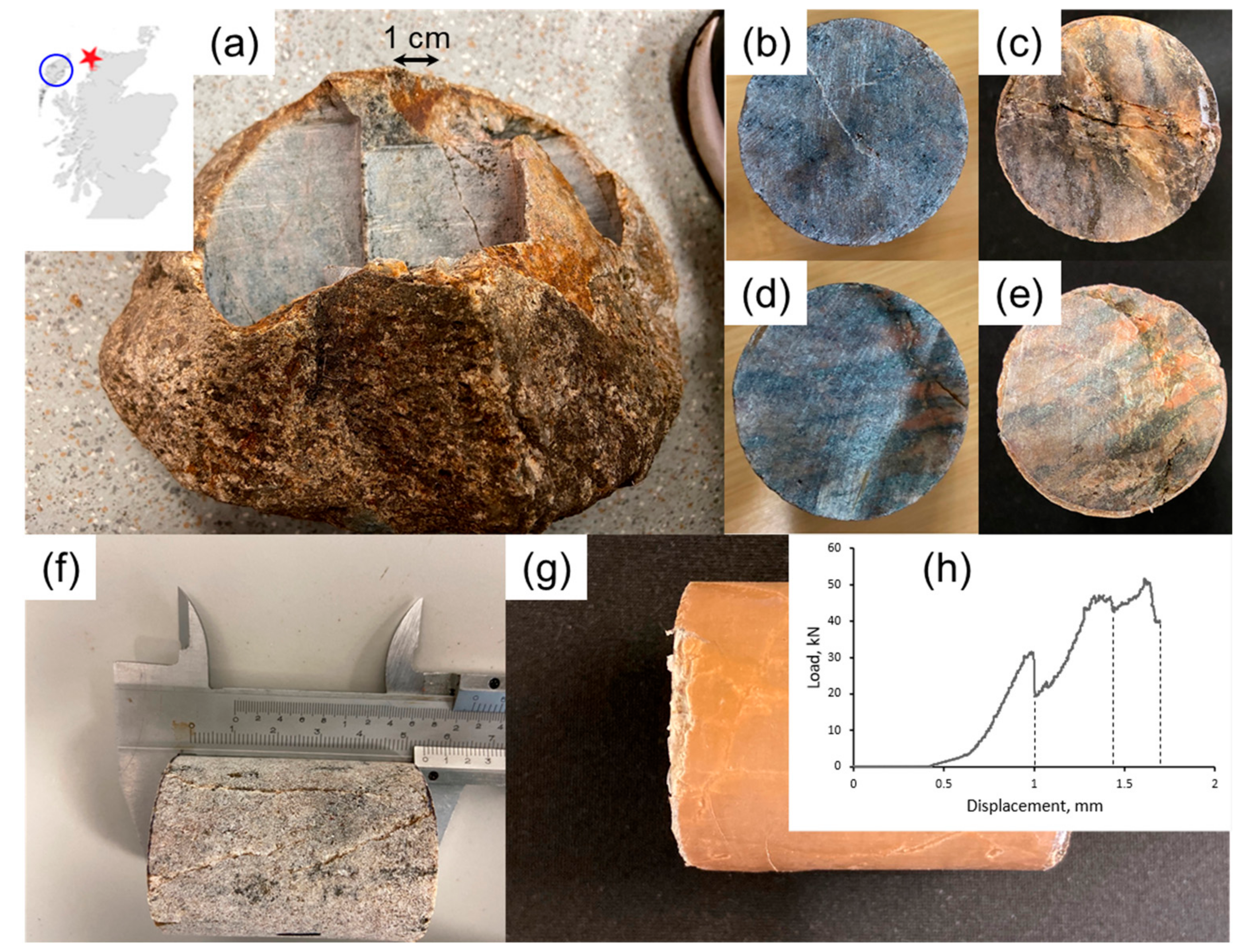
2. Materials and Methods

The rock sample used in this study was cored from a weathered gneiss boulder collected from the Precambrian Lewisian Gneiss Complex in Northwest Scotland, near Clashnessie. The cylindrical rock sample (38 mm diameter, 54 mm length) was subjected to uniaxial loading under controlled stress and artificially fractured along pre-existing cracks. To preserve the cylindrical shape of the sample, it was wrapped in duct tape during the loading. The initial and final state of the sample is shown in Figure 1.

To mimic the fluids expected to saturate the fractured aquifer in similar conditions as encountered at the site where the sample was taken, i.e., in a coastal setting of NW Scotland, we used four aqueous solutions to measure the streaming potential coupling coefficient: (1) the artificial groundwater (AGW) comprising the main salts, consistent with the groundwater chemical composition as reported by BGS [36] for groundwater samples taken from similar Lewisian gneiss on the Isle of Harris (about 50 km West of the site, blue circle in Figure 1a; (2) the artificial seawater (ASW) formulated from the main ionic species; (3) low-salinity NaCl (LS); (4) high-salinity NaCl (HS) solutions. The ionic strength of LS and AGW was 7.35 × 10⁻³ M (M = moL·L⁻¹), while the ionic strength of HS and ASW was 0.7 M, hence the ionic strengths of NaCl and the corresponding complex solution were identical between all low- and all high-salinity experiments. Therefore, the impact of ionic strength on the zeta potential measured with NaCl in comparison with complex solutions was eliminated to isolate the effect of the chemical composition. The ionic composition and equilibrium pH of all solutions used in this study are presented in

Table 1. Chemical composition, equilibrium pH and electrical conductivity of tested solutions. The solution pH was measured using Mettler Toledo FiveGo pH meter, the electric conductivity of all solutions was measured using Jenway 4520 conductivity meter with the corresponding errors reflecting the instrument inaccuracy and measurement repeatability. AGW and LS solutions were prepared from high-salinity stock solutions of 0.735 M ionic strength, hence, errors in molar concentrations of all four tested solutions resulting from inaccuracies in weighing of the constituent salts are estimated at ± 3% of the reported values.

	AGW	LS	ASW	HS
[Na+], M	1.522 × 10−3	7.350 × 10−3	0.512	0.700
[Ca2+], M	1.612 × 10−3	-	0.013	-
[Mg2+], M	0.288 × 10−3	-	0.042	-
[Cl−], M	5.072 × 10−3	7.350 × 10−3	0.577	0.700
[SO42−], M	0.125 × 10−3	-	0.022	-
pH	6.0 ± 0.1	6.5 ± 0.1	6.2 ± 0.1	6.9 ± 0.1
${\sigma }_w$, S∙m−1	0.069 ± 0.001	0.097 ± 0.001	5.83 ± 0.01	6.13 ± 0.01
Ionic strength, M	7.350 × 10−3	7.350 × 10−3	0.700	0.700

.

To characterize the chemistry and mineralogy of the gneiss sample used in our experiments, XRD analysis was carried out on powdered offcuts. Moreover, a chip from the sample was polished to produce a thin section, which was analyzed using scanning electron microscopy (SEM). The main constituent minerals from the SEM analysis were identified to be: quartz (c. 35 wt.%), Na-feldspars (plagioclase including albite, c. 60 wt.% in total) and micas (muscovite and biotite, c. 5 wt.% in total). These mineral proportions are characteristic of felsic Lewisian gneiss, as previously reported (e.g., [37,38]).

Prior to the streaming potential measurements, the rock sample was cleaned using deionized water and methanol following the procedure described by Alroudhan et al. [39]. Note that the cleaning procedure did not have any noticeable effect on the sample, as measurements of the zeta potential and permeability were repeated several times after cleaning and returned the same values within the experimental uncertainty. Subsequently, the sample was saturated with the solution of interest and placed in a vacuum oven for 24 h to establish 100% of water saturation. The saturated rock sample was mounted in a core holder made of PEEK, similar to that described in detail by Vinogradov et al. [31]. The experimental setup used in this study, including a pair of Ag/AgCl external electrodes used to measure the streaming potential, was the same as the one reported in previous studies by Vinogradov and co-workers (e.g., [33]).

We used the paired-stabilized (PS) method [40] to measure the streaming potential coupling coefficient, from which the zeta potential was interpreted using the Helmholtz-Smoluchowski equation (e.g., [41]) and assuming negligible contribution of the surface electrical conductivity to the effective electrical conductivity of the aqueous solution occupying a mm-scale fracture (as discussed in subsequent sections):

$$C_{SP}={\left.\frac{{∆}V}{{∆}P}\right|}_{j=0}=\frac{\epsilon \zeta }{\mu {\sigma }_w}$$

(1)

where C_SP [V/Pa] is the streaming potential coupling coefficient calculated from the measured voltage DV [V] and the pressure difference DP [Pa] across the sample when the total current density j [A/m²] is zero; $\epsilon$ [F/m] is the permittivity of water; $\zeta$ [V] is the zeta potential; $\mu$ [Pa·s] is the dynamic viscosity of water; and ${\sigma }_w$ [S/m] is the electrical conductivity of the aqueous solution. Each measurement of the streaming potential coupling coefficient was carefully analyzed for potential error sources including voltage noise level, stability of voltage during the experiment and repeatability. The resulting cumulative errors are presented by the individual error bars in Figure 2, Figure 3 and Figure 4, as discussed below (all data accompanied by examples of SP experiment and error analysis are provided in S2 of the Supplementary Material).

Figure 2. Zeta potential of gneiss samples compared with published data on other types of rocks. Circles denote NaCl solutions, triangles correspond to AGW and squares are ASW. Filled symbols correspond to confining pressure of 7 MPa. Low ionic strength is denoted by blue symbols while the high ionic strength data corresponds to red symbols. The solid lines that outline domains of reported data for carbonates and sandstones are based on the published data summarized in Table 2.

Figure 2. Zeta potential of gneiss samples compared with published data on other types of rocks. Circles denote NaCl solutions, triangles correspond to AGW and squares are ASW. Filled symbols correspond to confining pressure of 7 MPa. Low ionic strength is denoted by blue symbols while the high ionic strength data corresponds to red symbols. The solid lines that outline domains of reported data for carbonates and sandstones are based on the published data summarized in Table 2.

Table 2. Summary of experimentally measured zeta potential in relevant samples saturated with NaCl and natural solutions. In the table, LS and HS correspond to low-salinity and high-salinity data, SS stands for sandstones, SP corresponds to sand packs, LS refers to limestones, SW is natural seawater from southern UK, TW is tap water and ALSW is artificial low-salinity water. Exact values of ionic strength in the table vary between 0.001 M and 0.01 M for low salinity, and between 0.5 M and 0.75 M for high-salinity data. For details, refer to the cited papers. The data sources are: a—Vinogradov et al. [31]; b—Walker and Glover [32]; c—Jaafar et al. [42]; d—Vinogradov et al. [43]; e—Vinogradov and Jackson [44]; f—Li et al. [45]; g—Tosha et al. [35]; h—Reppert and Morgan [46]; i—Morgan et al. [47]; j—Ishido and Mizutani [48]; k—Al Mahrouqi et al. [34]; l—Jackson et al. [49]; m—Collini et al. [50]; n—Heberling et al. [51]; o—Heberling et al. [52].

Sample; Mineralogy	Solution	Zeta Potential, mV		Source
		LS	HS
Grey shaded area
Fontainebleau SS; >99% quartz	NaCl	−52	−20	a, b
Lochaline SS; >99% quartz	NaCl	−77	−25	b
Stainton SS; 90% quartz, 5% clays and feldspar	NaCl	−26	−16	a
St Bess SS; 90% quartz, <5% clays	NaCl	−31	−16	a, c
St Bees SS; 90% quartz, <5% clays	SW	N/A	−13	a
Doddington SS; 69% quartz, 5% clays	NaCl	−22	−10	e
SP; >99% quartz	TW	−100	N/A	a
SP; >99% quartz	NaCl	−20	−12	d
Berea SS; 90% quartz, up to 4% clays	NaCl	−20	−17	f
Boise SS; 47% quartz, 26% plagioclase, 3% clays	NaCl	−20	−20	b
Inada granite; N/A	KCl	−35	N/A	g
Westerly granite, 38% plagioclase 29% quartz	NaCl	−20	N/A	h
Crushed Westerly granite; N/A	KCl/NaCl	−65	N/A	i
Inada granite; N/A	KNO3	−70	N/A	j
White shaded area
Ketton LS; 97% calcite, 3% dolomite	NaCl	N/A	−6	k
Estaillades LS; 95% calcite, 4% dolomite, 1% anhydrite	NaCl	N/A	−6	k
Portland LS; 96.6% calcite, 3.4% quartz	NaCl	N/A	−9	k
Estaillades LS; 95% calcite, 4% dolomite, 1% anhydrite	SW	N/A	−1.25	l
Reservoir BA LS; N/A	ALSW	−4	N/A	m
Reservoir BD LS; N/A	ALSW	−10	N/A	m
Outcrop TE LS; >99% calcite	Artificial	−15	−2	m
Crushed Iceland spar; 100% calcite	NaCl	−5 [n]	+4 [o]	n, o

Table 2. Summary of experimentally measured zeta potential in relevant samples saturated with NaCl and natural solutions. In the table, LS and HS correspond to low-salinity and high-salinity data, SS stands for sandstones, SP corresponds to sand packs, LS refers to limestones, SW is natural seawater from southern UK, TW is tap water and ALSW is artificial low-salinity water. Exact values of ionic strength in the table vary between 0.001 M and 0.01 M for low salinity, and between 0.5 M and 0.75 M for high-salinity data. For details, refer to the cited papers. The data sources are: a—Vinogradov et al. [31]; b—Walker and Glover [32]; c—Jaafar et al. [42]; d—Vinogradov et al. [43]; e—Vinogradov and Jackson [44]; f—Li et al. [45]; g—Tosha et al. [35]; h—Reppert and Morgan [46]; i—Morgan et al. [47]; j—Ishido and Mizutani [48]; k—Al Mahrouqi et al. [34]; l—Jackson et al. [49]; m—Collini et al. [50]; n—Heberling et al. [51]; o—Heberling et al. [52].

Sample; Mineralogy	Solution	Zeta Potential, mV		Source
		LS	HS
Grey shaded area
Fontainebleau SS; >99% quartz	NaCl	−52	−20	a, b
Lochaline SS; >99% quartz	NaCl	−77	−25	b
Stainton SS; 90% quartz, 5% clays and feldspar	NaCl	−26	−16	a
St Bess SS; 90% quartz, <5% clays	NaCl	−31	−16	a, c
St Bees SS; 90% quartz, <5% clays	SW	N/A	−13	a
Doddington SS; 69% quartz, 5% clays	NaCl	−22	−10	e
SP; >99% quartz	TW	−100	N/A	a
SP; >99% quartz	NaCl	−20	−12	d
Berea SS; 90% quartz, up to 4% clays	NaCl	−20	−17	f
Boise SS; 47% quartz, 26% plagioclase, 3% clays	NaCl	−20	−20	b
Inada granite; N/A	KCl	−35	N/A	g
Westerly granite, 38% plagioclase 29% quartz	NaCl	−20	N/A	h
Crushed Westerly granite; N/A	KCl/NaCl	−65	N/A	i
Inada granite; N/A	KNO3	−70	N/A	j
White shaded area
Ketton LS; 97% calcite, 3% dolomite	NaCl	N/A	−6	k
Estaillades LS; 95% calcite, 4% dolomite, 1% anhydrite	NaCl	N/A	−6	k
Portland LS; 96.6% calcite, 3.4% quartz	NaCl	N/A	−9	k
Estaillades LS; 95% calcite, 4% dolomite, 1% anhydrite	SW	N/A	−1.25	l
Reservoir BA LS; N/A	ALSW	−4	N/A	m
Reservoir BD LS; N/A	ALSW	−10	N/A	m
Outcrop TE LS; >99% calcite	Artificial	−15	−2	m
Crushed Iceland spar; 100% calcite	NaCl	−5 [n]	+4 [o]	n, o

Figure 3. Impact of ionic strength on the zeta potential measured on Lewisian gneiss sample saturated with (a) AGW and ASW, and (b) with NaCl solutions. For comparison, empirical linear regressions for clean sandstones (>95% quartz; [31]) and carbonates saturated with equilibrated NaCl solutions [34] are shown in green and black dashed lines, respectively. Filled symbols correspond to the confining pressure of 7 MPa. Green circles represent zeta potentials measured in Berea sandstone saturated with NaCl solutions and averaged over seven samples (right vertical axis); the black circles correspond to results obtained with Berea sandstones saturated with CaCl₂ solutions and averaged over six samples [45].

Figure 3. Impact of ionic strength on the zeta potential measured on Lewisian gneiss sample saturated with (a) AGW and ASW, and (b) with NaCl solutions. For comparison, empirical linear regressions for clean sandstones (>95% quartz; [31]) and carbonates saturated with equilibrated NaCl solutions [34] are shown in green and black dashed lines, respectively. Filled symbols correspond to the confining pressure of 7 MPa. Green circles represent zeta potentials measured in Berea sandstone saturated with NaCl solutions and averaged over seven samples (right vertical axis); the black circles correspond to results obtained with Berea sandstones saturated with CaCl₂ solutions and averaged over six samples [45].

Figure 4. Impact of the confining pressure on the zeta potentials measured on Lewisian gneiss sample saturated with aqueous solutions of 0.007 M (a) and 0.7 M (b) ionic strength. The dotted horizontal lines demonstrate that the zeta potentials were identical (within the experimental uncertainty) across the salinity range.

Figure 4. Impact of the confining pressure on the zeta potentials measured on Lewisian gneiss sample saturated with aqueous solutions of 0.007 M (a) and 0.7 M (b) ionic strength. The dotted horizontal lines demonstrate that the zeta potentials were identical (within the experimental uncertainty) across the salinity range.

To replicate different depth of fractured gneiss of the aquifer of interest and, hence, different fracture aperture, two different confining pressures were tested with all four solutions: 4 MPa and 7 MPa.

3. Results and Discussion

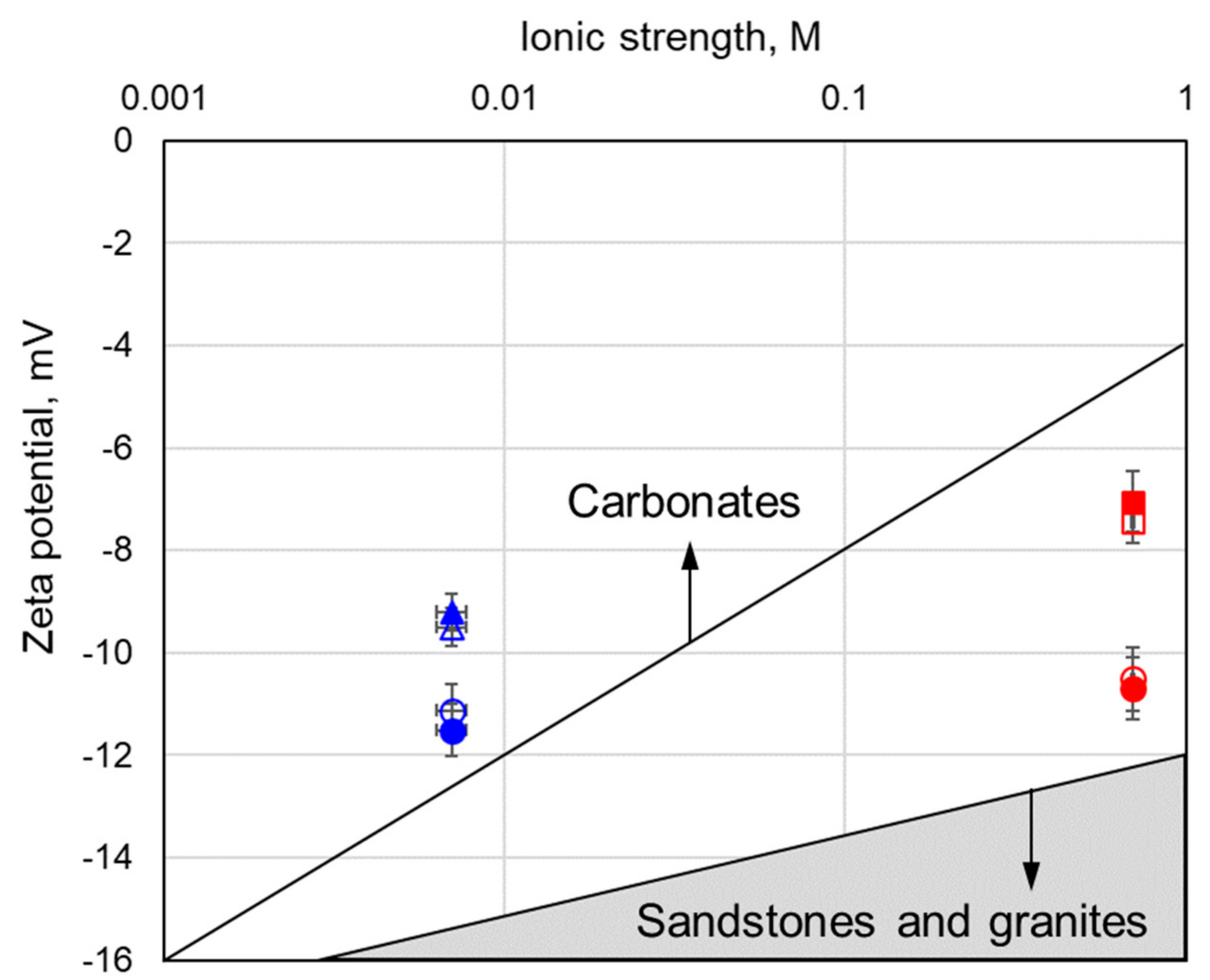
3.1. Effect of Rock Type and Mineralogy

We begin with comparing the zeta potentials measured in the fractured gneiss sample against published data on pure sandstone (>99% quartz), clayey sandstone (2–5% clay content), sand packs (>99% quartz), carbonate (>95% calcite) and granite samples saturated with aqueous solutions of similar ionic strength and composition, and under equilibrium conditions (i.e., rock samples were thoroughly equilibrated with aqueous solutions). The results presented in Figure 2 indicate that the zeta potentials measured with gneiss saturated with high-salinity electrolytes were generally more negative compared with values obtained in carbonates saturated with aqueous solutions of ionic strengths within the range of those tested in this study, and were more positive across the salinity range compared with the data from sand packs, as well as from clean and clayey sandstones. All of our results in Figure 2 are color-coded with red symbols denoting the ionic strength of 0.7 M and the blue symbols corresponding the ionic strength of 7.35 × 10⁻³ M.

The individual data points included in the grey and white shaded areas are summarized in Table 2, for which zeta potentials measured in intact and crushed sandstone, carbonate and granite samples have been reported. To the best of our knowledge, there have been no published data on zeta potentials measured with basement rocks (e.g., granite or gneiss) saturated with high ionic strength electrolytes, hence, the corresponding column is populated with N/A (not available).

The majority of the data detailed in Table 2 indicate that the zeta potentials of gneiss saturated with high-salinity solutions (0.7 M) are negative and larger in magnitude compared with carbonates, but smaller in magnitude compared with sandstones. However, there are two exceptions, with the zeta potential of −10 mV measured in Doddington sandstone saturated with 0.5 M NaCl solution, and the zeta potential of −9 mV measured in Portland limestone saturated with equilibrated 0.5 M NaCl solution, both of which are comparable with the values obtained for the gneiss sample saturated with ASW. We attribute these anomalous reported zeta potentials to a higher clay content in the Doddington sample and quartz inclusion in the Portland limestone, which made these samples’ response to 0.5 M NaCl solutions to be dissimilar to that of pure silica or calcite rocks, but comparable with the signal measured with gneiss.

On the other hand, the zeta potentials in the gneiss sample saturated with low-salinity electrolytes (7.35 × 10⁻³ M) were found to be more positive compared with both sandstone and carbonate samples, with the exception of −5 mV recorded with crushed Iceland spar saturated with 0.01 M NaCl mixed with 1 mM CaCl₂ solution [51], and −4 mV measured in reservoir carbonate sample BA of unknown mineralogy saturated with artificial 0.01 M electrolyte containing Ca²⁺ and Mg²⁺ [50]. The results with Iceland Spar were obtained at an unconfirmed chemical equilibrium with solutions and showed strong dependence on the concentration of added CaCl₂, so that the measured zeta potential varied between −3 mV with 5 mM of CaCl₂ and −14 mV with 0.1 mM of CaCl₂, thus, limiting the applicability of direct comparison between our results and those reported by Heberling et al. [51]. In contrast, the results reported by Collini et al. [50] were obtained under equilibrium conditions, but the solution used by the authors contained a considerable amount of Mg²⁺ (1 mM), Ca²⁺ (0.3 mM) and no SO₄²⁻ in their 0.01 M solution. It is generally agreed that divalent ions act as potential determining ions (PDIs) for clays (e.g., [53]), so that divalent cations make the zeta potential more positive while divalent anions tend to make the zeta potential more negative. Hence, in absence of SO₄²⁻ in the tested low-salinity solution, the presence of Ca²⁺ and Mg²⁺ made the zeta potential more positive compared with pure NaCl and seawater in sandstones, other carbonates or gneiss.

There have been numerous reported measurements of the zeta potential in carbonate samples (e.g., refer to Figure 3 in Jackson et al. [23]) and the values in these studies ranged between −20 mV and +20 mV for low-salinity (ionic strength below 0.01 M) solutions with pH of 7. However, as discussed by Al Mahrouqi et al. [34], none of these measurements were conducted under conditions of thermo-chemical equilibrium between the tested solutions and rock minerals, hence, these data cannot be directly compared with our results.

Moreover, considering the mineralogy of our gneiss sample, we have found a limited number of published studies reporting measurements of the zeta potential of plagioclase [54] including albite [55], muscovite [56] and biotite [57]. None of these studies conducted their electrophoretic mobility measurements under equilibrium conditions, hence, the tested minerals could dissolve during the experiments with single salt aqueous solutions. This situation would be similar to that reported by Alroudhan et al. [39] and Al Mahrouqi et al. [34] for carbonate samples, or the one reported by Reppert and Morgan [46] for granite, all of which observed varying zeta potential during their experiments until it stabilized at the final equilibrium value after hundreds of hours of equilibration. Therefore, the measured zeta potentials of plagioclase, albite, biotite and muscovite systems could not be compared with our data and between each other in any other way, but qualitatively. Furthermore, it is worth noting that the scarce data available for these minerals cannot be utilized for interpreting the SP signal measured in fractured gneiss aquifers, which are expected to be fully equilibrated with aqueous solutions, thus emphasizing the importance of our laboratory results. The reported laboratory data on mica and feldspar minerals generally suggest that the zeta potentials remain negative across the pH range of interest (6–8) but become progressively smaller in magnitude following the order: $\left|{\zeta }_{plagioclase}\right| < \left|{\zeta }_{albite}\right| \cong \left|{\zeta }_{biotite}\right| < \left|{\zeta }_{muscovite}\right|$ with the values reported for plagioclase ranging between −10 mV and +15 mV obtained with 10⁻² M di-sodium tetraborate solution [54].

All in all, our experimental results demonstrated that all zeta potentials of Lewisian gneiss, saturated with low- to high-salinity aqueous solutions consisting of a single salt or a mixture of different salts, were unique. The main constituent minerals of this rock type are quartz, feldspar and mica, so the electrochemical response to ionic species in tested solutions is expected to reflect the individual contribution of each mineral. Since there are no reported zeta potential measurements of feldspars and micas in contact with various aqueous solutions at equilibrium conditions, we hypothesize that the electric surface charge on these complex minerals is controlled by multi-valent PDIs, similar to the mechanism of the surface charge development on calcite surface (e.g., [58]). Therefore, the resulting surface charge and the corresponding zeta potential of gneiss-hosted feldspars in our experiments caused the zeta potential to become less negative compared with pure quartz systems. Micas in contact with aqueous solutions ([55,56]) were reported to produce more negative zeta potential compared with feldspars ([54,57]). At the same time, the negative zeta potentials measured with micas were smaller in magnitude compared with negative values on silica surface, consistent with a published study of silica and mica minerals in contact with 10⁻³ M KCl solution [56]. Moreover, previously published studies also reported a shift in the zeta potentials towards more positive values with solutions containing divalent cations relative to NaCl/KCl measurements for all types of minerals, with a more pronounced shift reported with micas [59] and feldspars (comparing the results obtained with albite in contact with 10⁻³ M NaCl in Gülgönül et al. [60] vs. 10⁻³ M CaCl₂ in Demir et al. [61]) compared with pure quartz (e.g., [62]). Hence, the zeta potential in our experiments responded to changes in chemical composition in a fashion similar to that of calcite/mica/feldspar and became more positive with divalent cations, while the electric charge on the gneiss-hosted quartz surface sites was mostly controlled by pH, thus, remaining insensitive to changes in the electrolyte composition. Moreover, the uniqueness of the gneiss zeta potentials was demonstrated by the impact of varying ionic strength, which appeared to be less pronounced than that obtained with either carbonates or pure sandstones (>95% quartz). Both the impact of composition and ionic strength on the zeta potential in gneiss samples will be discussed in more detail in the subsequent section.

3.2. Effect of the Ionic Strength and Chemical Composition

It is generally agreed that zeta potential decreases in magnitude with increasing ionic strength as a result of a collapse of the electrical double layer (e.g., [63]) and our results with ASW and AGW, as shown in Figure 3a, were consistent with this behavior. The measured zeta potentials of these systems remained negative but became smaller in magnitude with increasing ionic strength. In contrast, the zeta potentials measured with NaCl solutions remained constant within the experimental uncertainty with increasing salinity, as demonstrated by the horizontal dash-dotted line in Figure 3b. Our results are denoted by the red and blue symbols in Figure 3.

As shown in Figure 3a, the rate at which the zeta potential decreases in magnitude with increasing salinity in gneiss samples (blue and red symbols) is significantly lower than that reported for clean sandstones (green dashed line) and carbonates (black dashed line) saturated with NaCl solutions. However, a recent study [45] reported an anomalous salinity dependence of the zeta potential in clayey Berea samples. In this study the zeta potential obtained with NaCl solutions varied from −18.3 mV at 0.005 M to −21.4 mV at 0.5 M (green circles in Figure 3), thus, indicating much weaker and reversed concentration dependence compared with that of clean sandstones. At the same time, the magnitude of zeta potential in Berea NaCl experiments remained significantly larger compared with our gneiss results. In contrast, the zeta potentials of approximately −7 ± 0.3 mV measured in Berea-CaCl₂ systems (black circles in Figure 3) remained unchanged between ionic strength of 0.008 M and 0.8 M. In this sense, the independant of salinity zeta potential in the clayey sandstones saturated with CaCl₂ was qualitatively similar to the observed trend in the gneiss sample saturated with NaCl, but the magnitude of the latter was consistently larger.

The zeta potentials in our gneiss sample saturated with aqueous solutions of complex composition became more negative with decreasing salinity and was consistently more positive compared with the results obtained with NaCl. Moreover, the zeta potential of −7.2 ± 0.2 mV obtained with ASW (0.7 M) were comparable with those measured in Berea samples saturated with CaCl₂ (−7.0 ± 0.3 mV; [45]) and Portland limestone saturated with equilibrated NaCl (−8.0 ± 0.5 mV; [34]).

Figure 3 clearly indicates that zeta potentials of Lewisian gneiss saturated with aqueous solutions are unique in their response to varying ionic strength and brine composition. These observations suggest that gneiss mineralogy affects the zeta potential that strongly responds to presence of divalent ions, hence Ca²⁺, Mg²⁺ and SO₄²⁻ are PDIs for this rock type, similar to the generally agreed feature of carbonates (Al-Mahrouqi et al. [34]), feldspars (Demir et al. [61]) and micas (Adamczyk et al. [59]). Therefore, accurate laboratory measurements of the zeta potential in gneiss should be carried out prior to attempting interpretation of filed SP data.

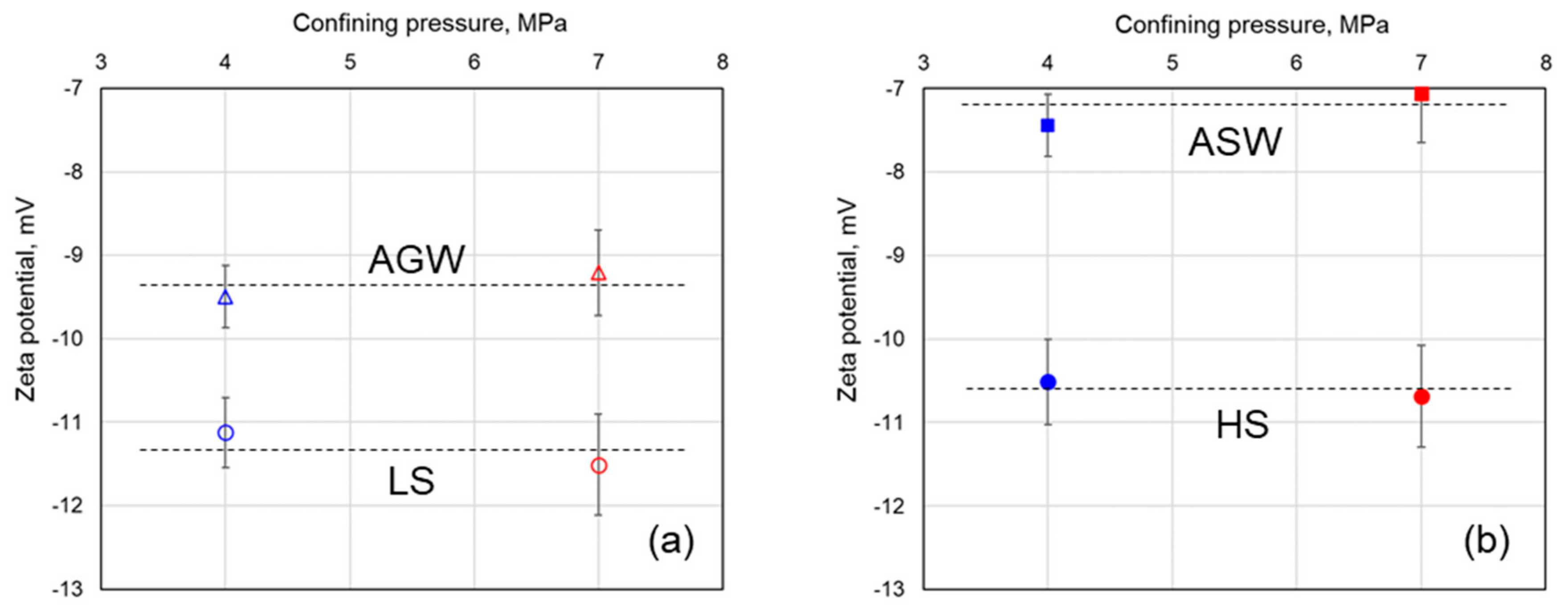
3.3. Effect of Confining Pressure

In all of our experiments, we observed the zeta potentials to be independent of the confining pressure (Figure 4). The increasing confining pressure applied to the fractured rock sample resulted in a decrease of the apparent permeability from 51 mD ($1 \mathrm{mD}\cong {10}^{-15} {\mathrm{m}}^2$) at 4 MPa to 43 mD at 7 MPa. The observed decrease in the permeability corresponds to a closure of the fracture, thus potentially leading to an increased effect of the surface electrical conductivity.

To quantify the effect of the confining pressure on the measured streaming potential coupling coefficient, zeta potential and the fracture aperture, we considered the following geometry of the investigated rock sample (Figure 5).

All our streaming potential experiments were conducted under steady-state fluid flow conditions and the induced flow through the fracture was consistent with the direction of the rock sample. Therefore, for the geometry described in Figure 5 and the experimental conditions, the Navier–Stokes equations simplify to 1-D flow in the Cartesian coordinate system as follows:

$$\mu \frac{d^2{v}_x}{d{y}^2}=\frac{{∆}P}{L}$$

(2)

where $v_x\left(y\right)$ is the fluid velocity in x-direction inside the fracture. Applying the no-slip boundary conditions at both fracture walls, the fluid velocity profile is given by:

$$V_x=\frac{1}{2\mu }\frac{{∆}P}{L}\left(y^2-w^2\right)$$

(3)

Multiplying Equation (3) by the cross-section area to the flow, $2wH$, and integrating across the fracture aperture (between −w and +w) yields the well-known cubic law [64] for the total volumetric flow rate, Q:

$$Q=-\frac{2H{w}^3}{3\mu }\frac{{∆}P}{L}$$

(4)

Now, equating the flow rate given by Equation (4) with that from the Darcy’s law, $Q=-\frac{2kHw}{\mu }\frac{{∆}P}{L}$, the effective permeability is expressed as:

$$k=\frac{w^2}{3}$$

(5)

Equation (5) is consistent with a recently published study [65] in the limit of a single fracture, and it implies that for a decrease of approximately 16% in sample’s permeability (from 51 mD to 43 mD), the corresponding expected decrease in fracture aperture (2w) will be around 8% (from 0.782 mm at 4 MPa to 0.718 mm at 7 MPa). Decreasing fracture aperture implies a smaller distance of separation between the fracture walls, and as such, a higher confining pressure can potentially have an impact on the electrical properties of hydraulically active fractures via an increased impact of the surface electrical conductivity and the zeta potential.

To investigate the impact of fracture aperture on the electrokinetic properties of the sample, we consider the streaming current under the steady state experimental conditions and for geometry described in Figure 5:

$$I_s=2\underset{0}{\overset{w}{{\displaystyle \int }}}\Sigma \left(y\right)v_x\left(y\right)Hdy$$

(6)

where $\Sigma$ [C/m³] is the volumetric charge density. The flow of mobile excess counter-ions that contribute to the streaming current is confined to the diffuse part of the electrical double layer (EDL), which has a thickness of approximately 3 nm for 7.35 × 10⁻³ M and an even smaller thickness for higher salinity, so that the thickest expected EDL will still be two orders of magnitude smaller than the estimated fracture aperture. Therefore, we can use this condition to linearize the flow velocity that contributes to the streaming current in the region adjacent to the fracture walls, where $y\approx w$:

$$V_x=\frac{1}{2\mu }\frac{{∆}P}{L}\left(y^2-w^2\right)\approx \frac{1}{2\mu }\frac{{∆}P}{L}2w\left(y-w\right)$$

(7)

Introducing a new variable $\theta =y-w$, using Poisson equation for the charge density, $\Sigma =-\epsilon \frac{d^{2}V}{d{y}^2}$ (where V is the electric potential and $\epsilon$ is the permittivity of the aqueous solution), substituting Equation (7) into Equation (6), and integrating by parts yields an expression for the streaming current through the fracture:

$$I_s=-\frac{2wH\epsilon \zeta }{\mu }\frac{{∆}P}{L}$$

(8)

where $\zeta$ is the zeta potential at $y=\pm w$. We now apply the boundary conditions of zero net current coming in or out of the fracture, and no charge separation along the fracture. In such case, the streaming current must be balanced by the conduction current of equal magnitude and opposite direction. The conduction current is given by Ohm’s law:

$$I_c=2wH{\sigma }_w\frac{{∆}V}{L}+2H{\sigma }_s\frac{{∆}V}{L}=2wH\frac{{∆}V}{L}\left[{\sigma }_b+\frac{{\sigma }_s}{w}\right]$$

(9)

where ${∆}V$ is the electric potential difference (voltage) across the fracture, ${\sigma }_w$ [S/m] is the electrical conductivity of the bulk aqueous solution and ${\sigma }_s$ [S] is the surface electrical conductivity due to the presence of EDL. Using the condition of electro-neutrality, $I_s=-I_c$, the streaming potential coupling coefficient can be expressed:

$$C_{SP}=\frac{{∆}V}{{∆}P}=\frac{\epsilon \zeta }{\mu \left[{\sigma }_w+\frac{{\sigma }_s}{w}\right]}$$

(10)

Note that Equation (10) explicitly expresses the effective electrical conductivity of brine with the contribution of the surface conductivity, but becomes equal to the Helmholtz-Smoluchowski equation (Equation (1)) when the surface conductivity is negligibly small. The zeta potential can now be expressed from the measured streaming potential coupling coefficient as:

$$\zeta =\frac{C_{SP}\mu \left[{\sigma }_w+\frac{{\sigma }_s}{w}\right]}{\epsilon }$$

(11)

For the two tested ionic strengths of 7.35 × 10⁻³ M and 0.7 M, the permittivity and viscosity of the NaCl solutions can be calculated using the approach described in Saunders et al. [28], while C_SP and the electric conductivity of the solutions were directly measured during the experiments. Rock, fluid and electrokinetic properties for all our NaCl experiments are summarized in

Table 3. Rock, fluid and electrokinetic properties of NaCl experiments at 7.35 × 10⁻³ M (LS) and 0.7 M (HS) ionic strengths. The confining pressure is denoted by P in the table and k is the measured absolute permeability. The fracture aperture (2w) is interpreted using Equation (5).

ID	P, MPa	$\mathit{\mu }$, Pa·s	$\mathit{\epsilon }$ F·m−1	${\mathit{C}}_{\mathit{S}\mathit{P}},\mathbf{mV}·{\mathbf{MPa}}^{-1}$	$\mathit{\zeta }$	k, mD	2w, nm
LS	4	9.33 × 10−4	7.00 × 10−10	−86.4	−11.12	51 ± 1	782
LS	7	9.33 × 10−4	7.00 × 10−10	−89.5	−11.51	43 ± 1	718
HS	4	9.89 × 10−4	6.97 × 10−10	−1.21	−10.52	51 ± 1	782
HS	7	9.89 × 10−4	6.97 × 10−10	−1.23	−10.69	43 ± 1	718

along with estimates of fracture aperture made using Equation (5).

The fracture aperture estimated from the sample permeability is consistent with the experimentally measured values reported for artificially fractured granite sample [66]. In their study, Luo et al. [66] reported the hydraulic aperture of order of 200 mm, which is three orders of magnitude larger than the values estimated for our sample using Equation (5). However, the values of hydraulic conductivity of 13 cm/s measured by Lou et al. [66], which translates into the permeability of c. 13 × 10⁶ mD, is identical to that predicted by Equation (5), thus validating our approach and estimates.

To assess the effect of the surface conductivity on the zeta potential, we used a model of the zeta potential of silica-NaCl systems [67], for which the expected surface conductivities for the two ionic strengths tested in our experiments were evaluated to be 3.0 × 10⁻⁹ S for 7.35 × 10⁻³ M, and 4.5 × 10⁻⁹ S for 0.7 M solution. To characterize the impact of the surface conductivity on the zeta potential, we used the dimensionless Dukhin number (Du), defined by $Du=\frac{{\sigma }_s}{w{\sigma }_w}$ for the fracture geometry described in Figure 5 [7]:

$$Du=\frac{{\sigma }_s}{w{\sigma }_w}$$

(12)

From the estimates of the fracture aperture and surface conductivity, and measured bulk solution conductivities, Du translates to 7.9 × 10⁻² for 7.35 × 10⁻³ M solutions at 4 MPa of confining pressure; 8.6 × 10⁻² for 7.35 × 10⁻³ M solutions at 7 MPa; 1.9 × 10⁻³ for 0.7 M solutions at 4 MPa and 2.0 × 10⁻³ for 0.7 M solutions at 7 MPa. All estimated Du for our experimental conditions clearly satisfied the condition for a negligibly small contribution of the surface conductivity to the total effective conductivity of an aqueous solution, hence, a negligible effect on the zeta potential: $Du\ll 1$. Therefore, for all tested solutions, the surface electrical conductivity could be neglected, and Equation (1) was appropriate for interpreting the zeta potential from the measured streaming potential coupling coefficient.

To evaluate the aquifer depths at which surface conductivity becomes significant, we considered a study [66] that reported a near-linear correlation between the confining pressure and the hydraulic aperture of an artificially fractured granite sample. Thus, using estimates of the surface conductivity value for low-salinity solutions (Table 3), we were able to evaluate the confining pressure and the corresponding aquifer depth, at which the surface conductivity becomes significant, satisfying the condition of $Du\approx 0.1$. The aperture that satisfies $Du=0.1$ was calculated to be 310 nm using Equation (12), and the corresponding confining pressure was found to be 3.8 MPa, corresponding to an aquifer depth of 380 m, which is significantly deeper than the typical useful (from a resource point of view) depth of fractured gneiss aquifers, which varies between a few meters and a few hundred meters. At these depths, the impact of the surface conductivity on the zeta potential becomes substantial, hence, appropriate care should be taken to interpret the SP and ERT field data.

Future experimental work will aim at acquiring additional zeta potential values in systems comprising other specimens of the Lewisian gneiss and confining pressures higher than 7 MPa. These experiments will complement the data reported here and expand the range of tested conditions not covered in this work, thus, further improving our understanding of the zeta potential at the gneiss-water interfaces under conditions relevant to naturally fractured systems. The results will also be used to inform future surface complexation and molecular dynamics simulation studies aimed at describing gneiss-water systems under realistic conditions.

4. Conclusions

We report measurements of the zeta potential carried out for the first time on a fractured Lewisian gneiss sample saturated with NaCl solutions, artificial groundwater (AGW), artificial seawater (ASW) and under 4 MPa and 7 MPa of confining pressure. The results show that:

• Zeta potentials of gneiss are unique and dissimilar to sandstones, carbonates and even to individual gneiss constitutive minerals, i.e., mica and feldspar.
• The negative zeta potential decreases with increasing salinity when the sample is saturated with AGW and ASW, but the rate of the decrease is smaller compared to any other mineral.
• The negative zeta potential is independent of salinity when using NaCl; this feature is similar to what was observed with clayey sandstone [45] but the zeta potential of gneiss was found to be more positive compared with clayey sandstones saturated with NaCl.
• Significant amounts of feldspar and mica present in our gneiss sample were found to be responsible for the high sensitivity of the sample to the presence of divalent ions (Ca²⁺, Mg²⁺ and SO₄²⁻) compared with quartz. Therefore, these ions were identified as PDIs for gneiss, making the sample respond to compositional and concentration variations in a fashion similar to that of carbonate samples.
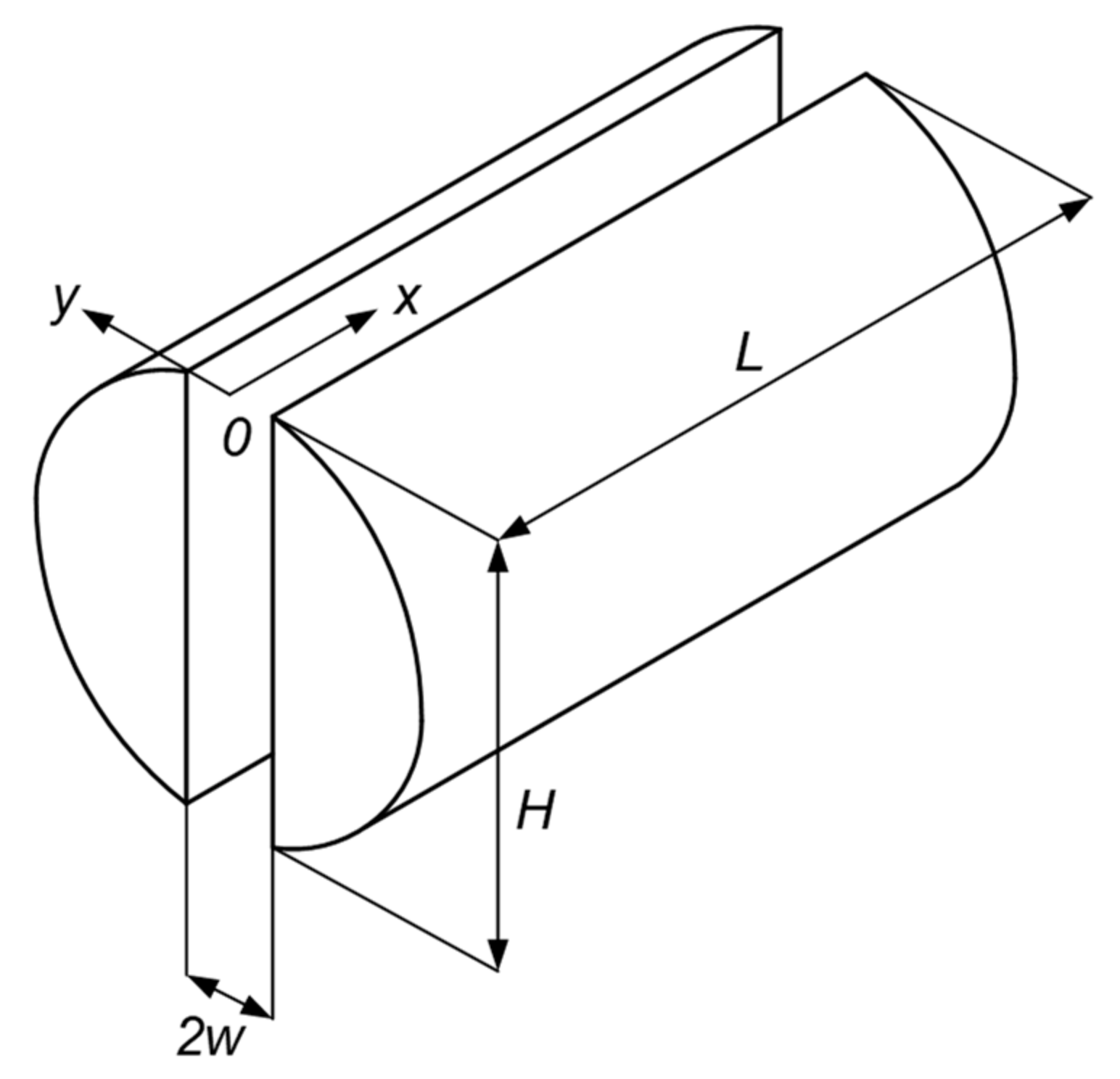
• The reported values of gneiss C_SP remained independent of the confining pressure, thus, suggesting that the surface electrical conductivity in gneiss aquifers could be neglected. A simple fracture model was developed to evaluate depths, and resulting in situ confining pressures, until which fracture aperture would remain large enough to neglect the surface electrical conductivity; this depth was found to be 380 m, which is much deeper than most water resources applications.

The reported dependence of the fractured gneiss zeta potential on confining pressure, composition and salinity of aqueous solutions can be used to identify newly formed fractures along naturally weathered pre-existing clacks from the measured signal, thus paving a way to a novel passive non-intrusive method of quantitative characterization of fracture network in crystalline rocks.

The above results suggest that interpretation of SP field data requires knowledge of the zeta potential values, which should be used to calculate C_SP using Equation (1). Subsequently, using the computed values of C_SP and voltages measured in the field, the expected pressure gradients can be quantified without any requirement of accounting for surface electrical conductivity. Finally, the obtained values of the pressure gradients will provide essential information on hydraulically active fractures (zero SP response results in zero pressure gradient, hence, implies no flow in that direction) and average fracture permeability (higher pressure gradients correspond to lower average fracture permeability).

References

1. Gustafson, G.; Krásný, J. Crystalline Rock Aquifers: Their Occurrence, Use And Importance. Hydrogeol. J. 1994, 2, 64–75. [Google Scholar] [CrossRef]
2. Ofterdinger, U.; MacDonald, A.M.; Comte, J.C.; Young, M.E. Groundwater in fractured bedrock environments: Managing catchment and subsurface resources–an introduction. Geol. Soc. Lond. Spec. Publ. 2019, 479, 1–9. [Google Scholar] [CrossRef] [Green Version]
3. Lachassagne, P.; Dewandel, B.; Wyns, R. Review: Hydrogeology of weathered crystalline/hard-rock aquifers—Guidelines for the operational survey and management of their groundwater resources. Hydrogeol. J. 2021, 29, 2561–2594. [Google Scholar] [CrossRef]
4. Bianchi, M.; MacDonald, A.M.; Macdonald, D.M.J.; Asare, E.B. Investigating the productivity and sustainability of weathered basement aquifers in tropical Africa using numerical simulation and global sensitivity analysis. Water Resour. Res. 2020, 56, e2020WR027746. [Google Scholar] [CrossRef]
5. Comte, J.-C.; Cassidy, R.; Nitsche, J.; Ofterdinger, U.; Pilatova, K.; Flynn, R. The typology of Irish hard-rock aquifers based on an integrated hydrogeological and geophysical approach. Hydrogeol. J. 2012, 20, 1569–1588. [Google Scholar] [CrossRef]
6. Roques, C.; Bour, O.; Aquilina, L.; Dewandel, B. High-yielding aquifers in crystalline basement: Insights about the role of fault zones, exemplified by Armorican Massif, France. Hydrogeol. J. 2016, 24, 2157–2170. [Google Scholar] [CrossRef]
7. Neuman, S.P. Trends, prospects and challenges in quantifying flow and transport through fractured rocks. Hydrogeol. J. 2005, 13, 124–147. [Google Scholar] [CrossRef]
8. Le Borgne, T.; Bour, O.; Paillet, F.; Caudal, J.-P. Assessment of preferential flow path connectivity and hydraulic properties at single-borehole and cross-borehole scales in a fractured aquifer. J. Hydrol. 2006, 328, 347–359. [Google Scholar] [CrossRef]
9. Krásný, J.; Sharp, J.M. Hydrogeology of fractured rocks from particular fractures to regional approaches: State-of-the-art and future challenges. In Groundwater of Fractured Rocks; Taylor and Francis: London, UK, 2007; pp. 1–32. [Google Scholar]
10. Becker, M.W.; Shapiro, A. Interpreting tracer breakthrough tailing from different forced-gradient tracer experiment configurations in fractured bedrock. Water Resour. Res. 2003, 39. [Google Scholar] [CrossRef] [Green Version]
11. Illman, W.A.; Liu, X.; Takeuchi, S.; Yeh, T.-C.J.; Ando, K.; Saegusa, H. Hydraulic tomography in fractured granite: Mizunami Underground Research site, Japan. Water Resour. Res. 2009, 45. [Google Scholar] [CrossRef] [Green Version]
12. Comte, J.-C.; Ofterdinger, U.; Legchenko, A.; Caulfield, J.; Cassidy, R.; González, J.A.M. Catchment-scale heterogeneity of flow and storage properties in a weathered/fractured hard rock aquifer from resistivity and magnetic resonance surveys: Implications for groundwater flow paths and the distribution of residence times. Geol. Soc. Lond. Spec. Publ. 2019, 479, 35–58. [Google Scholar] [CrossRef] [Green Version]
13. Hsieh, P. Scale Effects in Fluid Flow through Fractured Geologic Media. In Scale Dependence and Scale Invariance in Hydrology; Sposito, G., Ed.; Cambridge University Press: Cambridge, UK, 1998; pp. 335–353. [Google Scholar] [CrossRef]
14. Shapiro, A.M.; Ladderud, J.A.; Yager, R.M. Interpretation of hydraulic conductivity in a fractured-rock aquifer over increasingly larger length dimensions. Hydrogeol. J. 2015, 23, 1319–1339. [Google Scholar] [CrossRef]
15. Day-Lewis, F.D.; Slater, L.D.; Robinson, J.; Johnson, C.D.; Terry, N.; Werkema, D. An overview of geophysical technologies appropriate for characterization and monitoring at fractured-rock sites. J. Environ. Manag. 2017, 204, 709–720. [Google Scholar] [CrossRef]
16. González, J.A.M.; Comte, J.C.; Legchenko, A.; Ofterdinger, U.; Healy, D. Quantification of groundwater storage heterogeneity in weathered/fractured basement rock aquifers using electrical resistivity tomography: Sensitivity and uncer-tainty associated with petrophysical modelling. J. Hydrol. 2021, 593, 125637. [Google Scholar] [CrossRef]
17. Olsson, O.; Falk, L.; Forslund, O.; Lundmark, L.; Sandberg, E. Borehole radar applied to the characterization of hy-draulically conductive fracture zones in crystalline rock. Geophys. Prospect. 1992, 40, 109–142. [Google Scholar] [CrossRef]
18. Vouillamoz, J.; Lawson, F.; Yalo, N.; Descloitres, M. The use of magnetic resonance sounding for quantifying specific yield and transmissivity in hard rock aquifers: The example of Benin. J. Appl. Geophys. 2014, 107, 16–24. [Google Scholar] [CrossRef]
19. Wishart, D.N.; Slater, L.; Gates, A.E. Self potential improves characterization of hydraulically-active fractures from azimuthal geoelectrical measurements. Geophys. Res. Lett. 2006, 33. [Google Scholar] [CrossRef]
20. Wishart, D.N.; Slater, L.D.; Gates, A.E. Fracture anisotropy characterization in crystalline bedrock using field-scale azimuthal self potential gradient. J. Hydrol. 2008, 358, 35–45. [Google Scholar] [CrossRef]
21. Hasan, M.; Shang, Y.-J.; Jin, W.-J.; Akhter, G. Investigation of fractured rock aquifer in South China using electrical resistivity tomography and self-potential methods. J. Mt. Sci. 2019, 16, 850–869. [Google Scholar] [CrossRef]
22. Jackson, M.; Gulamali, M.Y.; Leinov, E.; Saunders, J.H.; Vinogradov, J. Spontaneous Potentials in Hydrocarbon Reservoirs During Waterflooding: Application to Water-Front Monitoring. SPE J. 2012, 17, 53–69. [Google Scholar] [CrossRef]
23. Jackson, M.; Butler, A.P.; Vinogradov, J. Measurements of spontaneous potential in chalk with application to aquifer characterization in the southern UK. Q. J. Eng. Geol. Hydrogeol. 2012, 45, 457–471. [Google Scholar] [CrossRef]
24. MacAllister, D.; Jackson, M.D.; Butler, A.P.; Vinogradov, J. Remote Detection of Saline Intrusion in a Coastal Aquifer Using Borehole Measurements of Self-Potential. Water Resour. Res. 2018, 54, 1669–1687. [Google Scholar] [CrossRef] [Green Version]
25. Roubinet, D.; Linde, N.; Jougnot, D.; Irving, J. Streaming potential modeling in fractured rock: Insights into the identi-fication of hydraulically active fractures. Geophys. Res. Lett. 2016, 43, 4937–4944. [Google Scholar] [CrossRef] [Green Version]
26. MacAllister, D.J.; Jackson, M.D.; Butler, A.P.; Vinogradov, J. Tidal influence on self-potential measurements. J. Geophys. Res. 2016, 121, 8432–8452. [Google Scholar] [CrossRef] [Green Version]
27. Graham, M.T.; MacAllister, D.; Vinogradov, J.; Jackson, M.D.; Butler, A.P. Self-Potential as a Predictor of Seawater Intrusion in Coastal Groundwater Boreholes. Water Resour. Res. 2018, 54, 6055–6071. [Google Scholar] [CrossRef] [Green Version]
28. Saunders, J.H.; Jackson, M.; Gulamali, M.; Vinogradov, J.; Pain, C. Streaming potentials at hydrocarbon reservoir conditions. Geophys. 2012, 77, E77–E90. [Google Scholar] [CrossRef] [Green Version]
29. Jackson, M.D.; Leinov, E. On the validity of the “thin” and “thick” double-layer assumptions when calculating streaming currents in porous media. Int. J. Geophys. 2012, 2012, 897807. [Google Scholar] [CrossRef] [Green Version]
30. MacAllister, D.; Graham, M.T.; Vinogradov, J.; Butler, A.P.; Jackson, M.D. Characterizing the Self-Potential Response to Concentration Gradients in Heterogeneous Subsurface Environments. J. Geophys. Res. Solid Earth 2019, 124, 7918–7933. [Google Scholar] [CrossRef] [Green Version]
31. Vinogradov, J.; Jaafar, M.Z.; Jackson, M. Measurement of streaming potential coupling coefficient in sandstones saturated with natural and artificial brines at high salinity. J. Geophys. Res. Space Phys. 2010, 115. [Google Scholar] [CrossRef] [Green Version]
32. Walker, E.; Glover, P.W.J. Measurements of the Relationship Between Microstructure, pH, and the Streaming and Zeta Potentials of Sandstones. Transp. Porous Media 2017, 121, 183–206. [Google Scholar] [CrossRef] [Green Version]
33. Hidayat, M.; Sarmadivaleh, M.; Derksen, J.; Vega-Maza, D.; Iglauer, S.; Vinogradov, J. Zeta potential of CO2-rich aqueous solutions in contact with intact sandstone sample at temperatures of 23 °C and 40 °C and pressures up to 10.0 MPa. J. Colloid Interface Sci. 2021, 607, 1226–1238. [Google Scholar] [CrossRef]
34. Al Mahrouqi, D.; Vinogradov, J.; Jackson, M.D. Zeta potential of artificial and natural calcite in aqueous solution. Adv. Colloid Interface Sci. 2017, 240, 60–76. [Google Scholar] [CrossRef] [PubMed] [Green Version]
35. Tosha, T.; Matsushima, N.; Ishido, T. Zeta potential measured for an intact granite sample at temperatures to 200 °C. Geophys. Res. Lett. 2003, 30, 1295. [Google Scholar] [CrossRef]
36. BGS. Final report on groundwater investigations on Harris. In British Geological Survey Commissioned Report Cr/01/69; BGS: Nottingham, UK, 2001. [Google Scholar]
37. Weaver, B.L.; Tarney, J. Lewisian gneiss geochemistry and Archaean crustal development models. Earth Planet. Sci. Lett. 1981, 55, 171–180. [Google Scholar] [CrossRef]
38. Macdonald, J.M.; Magee, C.; Goodenough, K. Dykes as physical buffers to metamorphic overprinting: An example from the Archaean–Palaeoproterozoic Lewisian Gneiss Complex of NW Scotland. Scott. J. Geol. 2017, 53, 41–52. [Google Scholar] [CrossRef] [Green Version]
39. Alroudhan, A.; Vinogradov, J.; Jackson, M. Zeta potential of intact natural limestone: Impact of potential-determining ions Ca, Mg and SO4. Colloids Surf. A Physicochem. Eng. Asp. 2016, 493, 83–98. [Google Scholar] [CrossRef] [Green Version]
40. Vinogradov, J.; Jackson, M. Multiphase streaming potential in sandstones saturated with gas/brine and oil/brine during drainage and imbibition. Geophys. Res. Lett. 2011, 38. [Google Scholar] [CrossRef]
41. Jouniaux, L.; Pozzi, J.-P. Streaming potential and permeability of saturated sandstones under triaxial stress: Consequences for electrotelluric anomalies prior to earthquakes. J. Geophys. Res. Space Phys. 1995, 100, 10197–10209. [Google Scholar] [CrossRef]
42. Jaafar, M.Z.; Vinogradov, J.; Jackson, M.D. Measurement of streaming potential coupling coefficient in sandstones saturated with high salinity NaCl brine. Geophys. Res. Lett. 2009, 36. [Google Scholar] [CrossRef]
43. Vinogradov, J.; Jackson, M.D.; Chamerois, M. Zeta potential in sandpacks: Effect of temperature, electrolyte pH, ionic strength and divalent cations. Colloids Surf. A Physicochem. Eng. Asp. 2018, 553, 259–271. [Google Scholar] [CrossRef]
44. Vinogradov, J.; Jackson, M.D. Zeta potential in intact natural sandstones at elevated temperatures. Geophys. Res. Lett. 2015, 42, 6287–6294. [Google Scholar] [CrossRef] [Green Version]
45. Li, S.; Collini, H.; Jackson, M.D. Anomalous Zeta Potential Trends in Natural Sandstones. Geophys. Res. Lett. 2018, 45, 11068–11073. [Google Scholar] [CrossRef]
46. Reppert, P.M.; Morgan, F.D. Temperature-dependent streaming potentials: 2. Laboratory. J. Geophys. Res. Space Phys. 2003, 108. [Google Scholar] [CrossRef]
47. Morgan, F.D.; Williams, E.R.; Madden, T.R. Streaming potential properties of westerly granite with applications. J. Geophys. Res. 1989, 94, 12449–12461. [Google Scholar] [CrossRef]
48. Ishido, T.; Mizutani, H. Experimental and theoretical basis of electrokinetic phenomena in rock-water systems and its applications to geophysics. J. Geophys. Res. Solid Earth 1981, 86, 1763–1775. [Google Scholar] [CrossRef]
49. Jackson, M.D.; Al-Mahrouqi, D.; Vinogradov, J. Zeta potential in oil-water-carbonate systems and its impact on oil recovery during controlled salinity water-flooding. Sci. Rep. 2016, 6, 37363. [Google Scholar] [CrossRef] [Green Version]
50. Collini, H.; Li, S.; Jackson, M.D.; Agenet, N.; Rashid, B.; Couves, J. Zeta potential in intact carbonates at reservoir conditions and its impact on oil recovery during controlled salinity waterflooding. Fuel 2020, 266, 116927. [Google Scholar] [CrossRef]
51. Heberling, F.; Trainor, T.P.; Lützenkirchen, J.; Eng, P.; Denecke, M.; Bosbach, D. Structure and reactivity of the calcite–water interface. J. Colloid Interface Sci. 2011, 354, 843–857. [Google Scholar] [CrossRef]
52. Heberling, F.; Klačić, T.; Raiteri, P.; Gale, J.D.; Eng, P.J.; Stubbs, J.E.; Gil-Díaz, T.; Begović, T.; Lützenkirchen, J. Structure and Surface Complexation at the Calcite(104)–Water Interface. Environ. Sci. Technol. 2021, 55, 12403–12413. [Google Scholar] [CrossRef]
53. Jackson, M.; Vinogradov, J.; Hamon, G.; Chamerois, M. Evidence, mechanisms and improved understanding of controlled salinity waterflooding part 1: Sandstones. Fuel 2016, 185, 772–793. [Google Scholar] [CrossRef] [Green Version]
54. Nyabeze, W.; McFadzean, B. Adsorption of copper sulphate on PGM-bearing ores and its influence on froth stability and flotation kinetics. Miner. Eng. 2016, 92, 28–36. [Google Scholar] [CrossRef]
55. Jie, Z.; Weiqing, W.; Jing, L.; Yang, H.; Qiming, F.; Hong, Z. Fe (III) as an activator for the flotation of spodumene, albite, and quartz minerals. Miner. Eng. 2014, 61, 16–22. [Google Scholar] [CrossRef]
56. Nishimura, S.; Tateyama, H.; Tsunematsu, K.; Jinnai, K. Zeta potential measurement of muscovite mica basal plane-aqueous solution interface by means of plane interface technique. J. Colloid Interface Sci. 1992, 152, 359–367. [Google Scholar] [CrossRef]
57. Bray, A.; Benning, L.G.; Bonneville, S.; Oelkers, E.H. Biotite surface chemistry as a function of aqueous fluid composition. Geochim. Cosmochim. Acta 2014, 128, 58–70. [Google Scholar] [CrossRef]
58. Vinogradov, J.; Hidayat, M.; Sarmadivaleh, M.; Derksen, J.; Vega-Maza, D.; Iglauer, S.; Jougnot, D.; Azaroual, M.; Leroy, P. Predictive surface complexation model of the calcite-aqueous solution interface: The impact of high concentration and complex composition of brines. J. Colloid Interface Sci. 2021; in press. [Google Scholar] [CrossRef] [PubMed]
59. Adamczyk, Z.; Zaucha, M.; Zembala, M. Zeta potential of mica covered by colloid particles: A streaming potential study. Langmuir 2010, 26, 9368–9377. [Google Scholar] [CrossRef] [PubMed]
60. Gülgönül, I.; Karagüzel, C.; Çınar, M.; Çelik, M.S. Interaction of Sodium Ions with Feldspar Surfaces and Its Effect on the Selective Separation of Na- and K-Feldspars. Miner. Process. Extr. Met. Rev. 2012, 33, 233–245. [Google Scholar] [CrossRef]
61. Demir, C.; Bentli, I.; Gülgönül, I.; Çelik, M. Effects of bivalent salts on the flotation separation of Na-feldspar from K-feldspar. Miner. Eng. 2003, 16, 551–554. [Google Scholar] [CrossRef]
62. Yukselen-Aksoy, Y.; Kaya, A. A study of factors affecting on the zeta potential of kaolinite and quartz powder. Environ. Earth Sci. 2010, 62, 697–705. [Google Scholar] [CrossRef]
63. Hunter, R.J. Zeta Potential in Colloid Science: Principles and Applications; Academic Press: New York, NY, USA, 1981. [Google Scholar]
64. Neuzil, C.E.; Tracy, J.V. Flow through fractures. Water Resour. Res. 1981, 17, 191–199. [Google Scholar] [CrossRef]
65. Thanh, L.; Jougnot, D.; Do, P.; Hue, D.; Thuy, T.; Tuyen, V. Predicting Electrokinetic Coupling and Electrical Conductivity in Fractured Media Using a Fractal Distribution of Tortuous Capillary Fractures. Appl. Sci. 2021, 11, 5121. [Google Scholar] [CrossRef]
66. Luo, J.; Zhu, Y.; Guo, Q.; Tan, L.; Zhuang, Y.; Liu, M.; Zhang, C.; Xiang, W.; Rohn, J. Experimental investigation of the hydraulic and heat-transfer properties of artificially fractured granite. Sci. Rep. 2017, 7, 39882. [Google Scholar] [CrossRef] [PubMed] [Green Version]
67. Leroy, P.; Devau, N.; Revil, A.; Bizi, M. Influence of surface conductivity on the apparent zeta potential of amor-phous silica nanoparticles. J. Colloid Interface Sci. 2013, 410, 81–93. [Google Scholar] [CrossRef] [PubMed] [Green Version]
Figure 1. Rock sample used in this study was cut from the weathered outcrop boulder (a) collected from the Clashnessie area denoted by the red star on the inset map (refer to the geological map of the area, S1, in the supplementary material); the core sample was naturally fractured as demonstrated by the top (b), bottom (d) and side (f) views; the sample was loaded along the longitudinal axis resulting in at least one fracture that extended from the top face (c) to the bottom one (e); to preserve its cylindrical shape during uniaxial loading, the sample was wrapped in duct tape (g) and experienced fracturing that corresponded to bulk displacements of 1 mm, 1.4 mm and 1.7 mm, as demonstrated by the load [kN] vs. displacement [mm] graph (h).
Applsci 12 00180 g001
Figure 5. The tested fractured rock sample is assumed to have a single fracture of aperture 2w, height H and length L.
Applsci 12 00180 g005