Abstract
Time series classification (TSC) task is one of the most significant topics in data mining. Among all methods for this issue, the deep-learning-based shows superior performance for its good adaption to raw series data and automatic extraction of features. However, rare eyes are kept on composing ensembles of these superior individual classifiers to achieve further breakthroughs. The existing deep learning ensembles NNE did a heavy work of combining 60 individuals but did not maximize the deserving improvement, since it merely pays attention to the diversity of individuals but ignores their accuracy. In this paper, we propose to construct an ensemble of Full Convolutional Neural Networks (FCN) by Random Subspace Method (RSM), named RSM-FCN. FCN is a simple but outstanding individual classifier and RSM is suitable for high dimensional data such as time series, but there are few instances. Thus, the combination of these strengths, RSM-FCN provides a highly cost-effective approach to yield promising results. Experiments on the UCR dataset demonstrate the effectiveness and reasonability of the proposed method.
1. Introduction
Time series classification (TSC) has attracted great attention, for it exists in a wide variety of fields [1], such as recognition and diagnosis problems in many industries, such as finance and medicine. Meanwhile, it is deemed as a challenging problem of data mining [2], due to its high dimensionality and nonalignment. These two drawbacks make it difficult to find distinctive features from time series.
To tackle this issue, hundreds of novel methods are proposed, including distance-based [3], feature-based, deep-learning-based [4] and ensemble-based. Wherein, methods based on deep learning shows impressive performance, as they have certain tolerance for the unaligned time series and be able to perceive the features benefiting for classification task automatically. An intuitional example is: Z. Wang [5], who evaluates some simple end-to-end deep learning benchmarks, which are Multilayer Perceptions (MLP), Residual Network (ResNet) and Fully Convolutional Network (FCN). The comparisons of experiment results show that FCN and ResNet outperform several complicated non-deep-learning TSC methods. The two winners, FCN and ResNet, are two specific forms of a Convolutional Neural Network (CNN). CNN is indeed the most highly regarded deep learning model in TSC field [4], and FCN is one of its common application forms. Ismail F. et al. [6] are attracted by the robustness and good performance of FCN, so that use it as the classifier to execute transfer learning experiments among datasets in UCR archive. Karim F et al. [7] employ FCN to perceive spatial features of time series curves, and augment it by adding LSTM module to extract time features simultaneously. Their proposed LSTM-FCN actually achieved the state-of-the-art performance at that time, while Elsayed N. et al. [8] use GRU module to realize the extraction of time-related features, and the GRU-FCN shows accurate results, as well. In fact, RNN modules like LSTM and GRU is not suitable for solving TSC problems alone [9], such superior results are mainly based on the contribution of FCN. Moreover, MFCN [10] is the proposed on the basis of FCN to learn multi-scale features of time series, and it also achieve improved performance. The successes of above models have repeatedly demonstrated the excellence of FCN for TSC problem.
Ensemble learning is an approach to achieve further improve the accuracy when basic model reaches its bottleneck. COTE [11] and PROP [12] are the representative in TSC field. One uses a total of 35 weak classifiers which trained by information from four domain to construct a strong one, the other integrates 11 kinds of classifiers which evaluates similarity by different distance measures. Except methods like those above, which combine different existing TSC techniques, classical ensemble learning ideas which provide heuristic rules for constructing diversity individual classifiers with given dataset are also employed. Ji Cv et al. [13] propose an XG-SF based on XGBoost algorithm and Shapelet features. Raza A. et al. [14] construct ensemble classifiers called EnRS-Bagging and EnRS-Boosting in a classical Boosting and Bagging manner, respectively. As we all know, the basic individual classifiers within ensemble model should be fine and diverse, whereas most of the mentioned methods employed the inferior decision tree or distance-based models, so that they cannot compete with state-of-the-art results, though achieve some improvements in accuracy. Furthermore, there is no method focuses on constructing deep neural network ensembles, until NNE [15] is proposed in 2019. NNE compose an ensemble of total 60 different neural networks that are generated by 6 kinds of models and 10 initial weights of each kind. It does pay attention to the diversity of individual classifiers but is not wise to involve the ones with more complex structure but less accurate judgment than FCN, such as Time-CNN [16] and MCD-CNN [17]. Which leads the achieved improvements not deserve the devoted efforts. Though NNE exceeds COTE [11] in accuracy under the contribution of huge amount basic classifiers, it does not maximally play the role of ensemble. In addition, approaches like XG-SF and EnRS are imperfect in another aspect that they did not choose the appropriate data perturbation method for time series. Methods such as Bagging will further lose the training instances and Boosting will be complex in fusion phase for multi-class problems, especially facing the datasets with dozens of categories.
Based on the above analysis, we propose to employ the simple-structure but excellent FCN and the classical data perturbation manner Random Subspace Method (RSM) [18] to build a deep learning ensemble. RSM, which samples in attributes subspaces, is appropriate for time series with high dimensionality except for a few instances. A classic example of RSM is the Machine Learning algorithm called Random Forest [18]. Other applications such as creating different subsets of the same features [19] or dataset [20] for sentiment classification and image classification support our task as well. However, differently than those discrete attributes or sets, the value-continuous and order-dependent time series cannot be randomly selected. Fortunately, the feature-based TSC solution Shapelet offers an inspiration. Shapelet views a high-dimensional time series as a combination of multiple shape primitives [21] and it learns several most discriminative primitives rather than whole series. Many Shapelet-based studies are proposed and achieve successes in TSC field, such as Shapelet Transformation [22], Logical Shapelet [23], as well as the COTE, XG-SF and EnRS, as mentioned before. Thus, it makes sense to only focus on the discriminative local information of time series. Despite its advantages, the brute force approach of Shapelet has a huge time complexity of O() [21], so we simulated but discarded the Shapelet method. Thus, in our method, the equally-divided time series intervals are regard as primitives.
Therefore, in this paper, a lightweight RSE-FCN (Random Subspace Ensembles of FCN) is designed to tackle the challenging TSC problem, where the equally-divided time series intervals are regarded as candidate subsequences, and Top-K ones with significantly discriminative feature are screened out by evaluation model, then with Random Subspace Method deploying on the Top-K and the superior FCN serving as individual classifier, the neural network ensembles RSE-FCN can be constructed. Through processes of screening and random selection, dimension of input can be reduced without losing discriminative features, so that FCN focusing on the key task-related information will be well trained. The basic classifier FCN has superior performance and the ensemble built by RSM will make a further breakthrough. Thus, promising results can be expected.
2. FCN Ensemble Built by Random Subspace Method
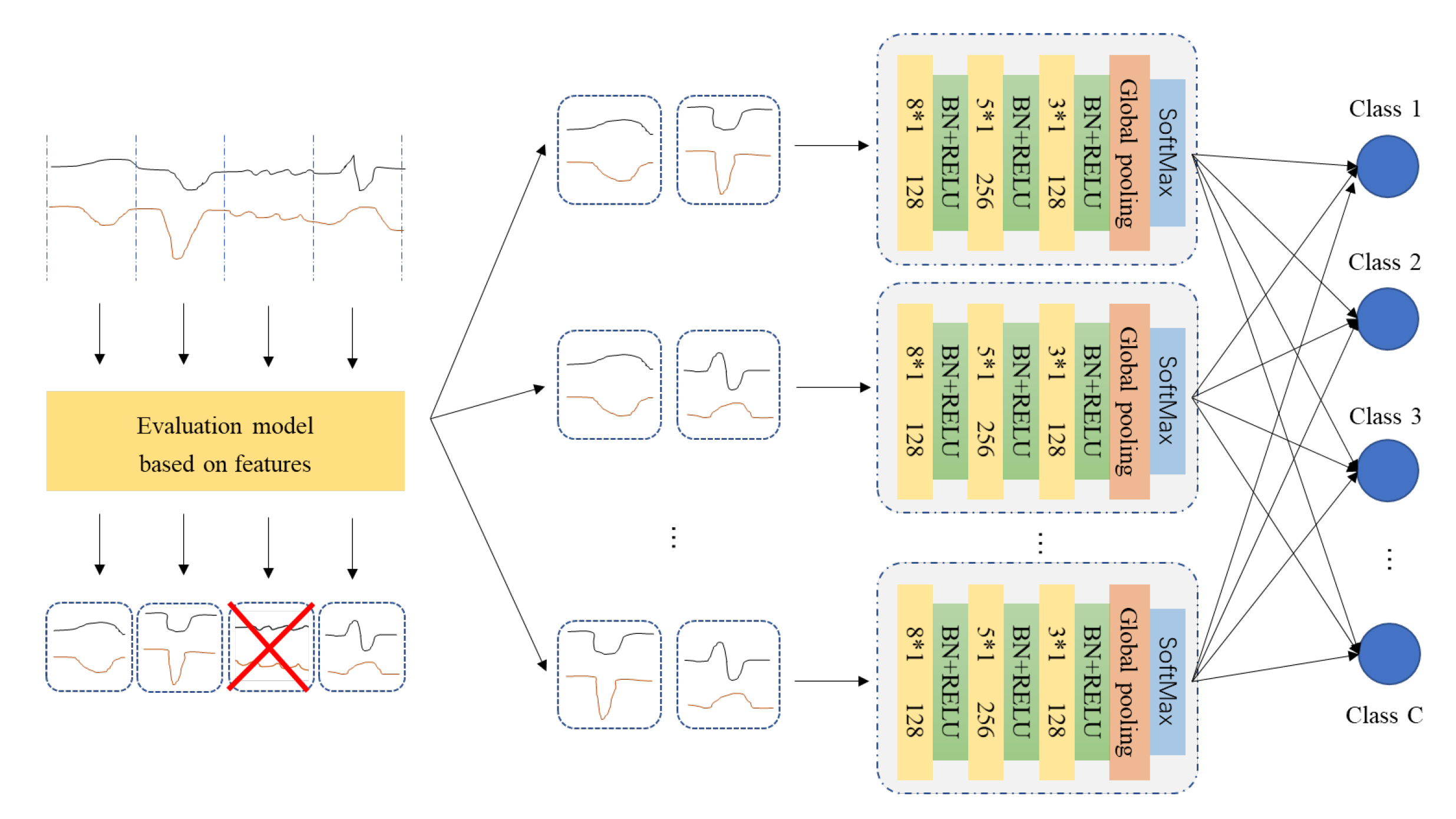
FCN has proven to be an effective vehicle for TSC problems. Ensemble learning is able to make further improvement from the accuracy level of single classifier. Furthermore, RSM prepares diverse individuals for ensemble by offering various combination of inputs. Meanwhile, classification model trained on the low-dimensional key features via screening, usually has good performance. This work proposes a Random Subspace Ensemble of FCN (RSE-FCN), combining the strength of above all, in order to yield promising TSC results. It converts raw continuous time series into discriminative subsequences, then deploys Random Subspace Method on these subsequences with FCN classifier. The overview of RSE-FCN is shown in Figure 1. In this section, we will first introduce the computationally less expensive converting method established by simulating Shapelet discovery, and then give a description of the precise working of proposed RSE-FCN.
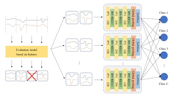
Figure 1.
The overall structure of RSE-FCN.
The procedure of Shapelet discovery can be summarized in four stages: enumerate candidate subsequences, evaluate candidates and form the Shapelet binary tuple, screen and re-rank. The converting operation adopted in our method generally follows the logic of Shapelet discovery. However, we rather to roughly eliminate part of irrelevant and redundant subsequences than to accurately search out K most representative primitives as Shapelet. As shown in Algorithm 1, first, N equally-divided intervals of time series are viewed as N candidate subsequences. Then, with classification accuracy as score, each subsequence is evaluated by a simple feature-based classifier. Here, roughly trained FCN are leveraged as the evaluator. Finally, K subsequences who have the highest score will be retained for Random Subspace Method.
| Algorithm 1. GetTopKBestSubsequences ( D, T, , , N, K). |
|
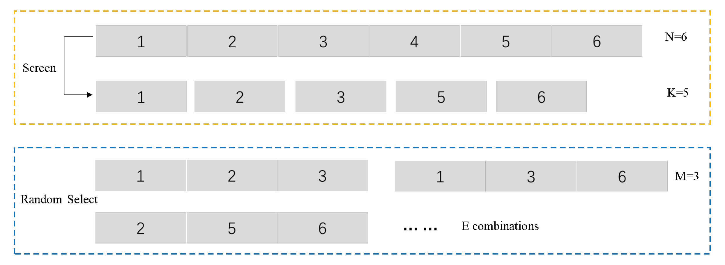
This ensemble framework requires four structural hyperparameters, they are: number of intervals to be divided N, number of optimal subsequences K, subsequences number M received by classifier and number of basic classifiers E. They directly correspond to the performance of proposed method. Figure 2 gives an example with hyperparameter value. A big N will lead each subsequence too short to be learned. The diversity of subsequence selections is positively related to N and the amount of individual classifiers E is also positively related to that diversity, so we think N and E within 10 is enough. Furthermore, obviously, M should be less than or equal to K. Moreover, M/N > 1/2 should be guaranteed, since above discovery process of key discriminative subsequence is rough, on the basis, retaining too little proportion as inputs may miss some beneficial features which hides in the discard ones.
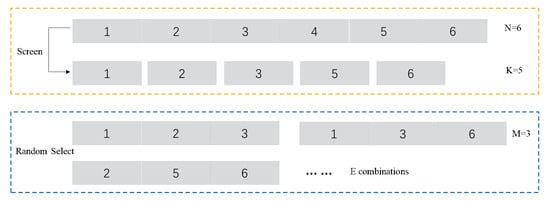
Figure 2.
Explanatory diagrams of the four hyperparameters.
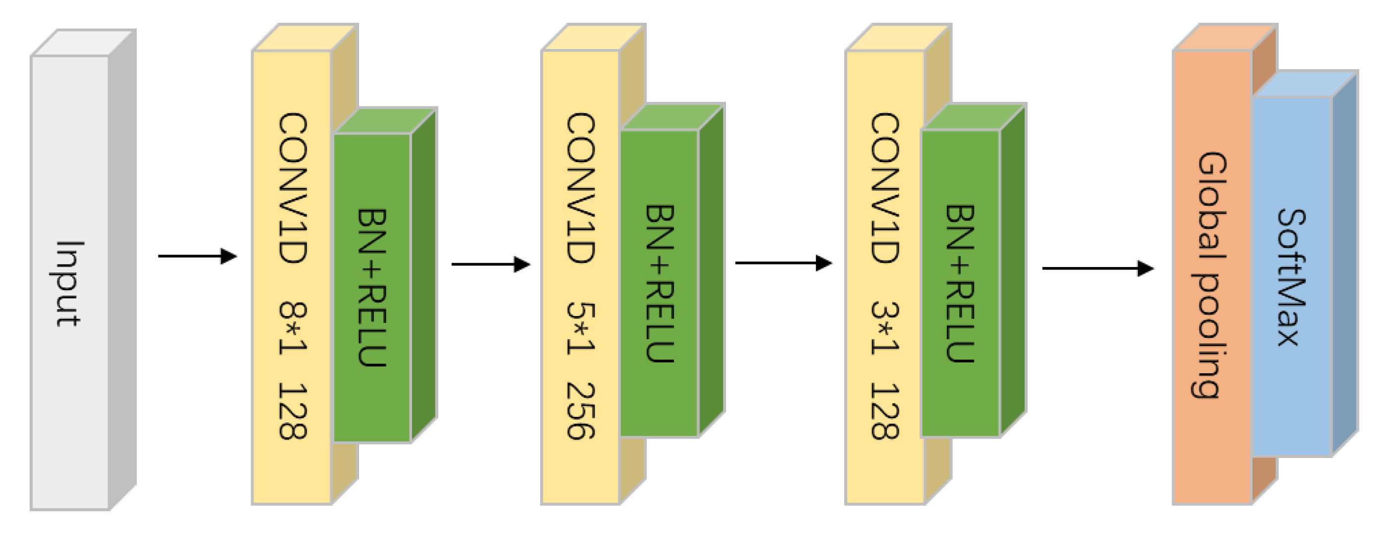
In the ensemble phase, Random Subspace Method is deployed on FCNs (Figure 3), which keeps the same structure with that found in another paper [5]. FCNs are trained by different combinations selected from top-K discriminative subsequences. Finally, the soft classification scores given by each individual classifier will be combined by soft voting.
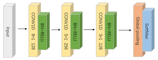
Figure 3.
The commonly used structure of FCN in TSC field.
Based on above settings and descriptions, the details of RSE-FCN can be presented in Algorithm 2. First, by GetTopKBestSubsequences method (Algorithm 1), KBestId, the set of ordinal number corresponding to K optimal intervals, can be obtained. The sets of N intervals Ds and Ts, which the train set D and test set T are divided into, should be reserved. Second, M ordinal numbers RsID are randomly selected out from KBestId every time and this operation should be repeated for E times. Next, according to Ds, Ts and current RsID, new training set D’ and test set T’ can be generated. To preserves the features which stretch over division nodes, the subsequences combining order should be in accordance with the number-ascending order rather than the selection order. Or reversely, we can get rid of the subsequences whose ordinal number not in the selected M ones from the interval sets of whole time series. Then, FCN is trained by current dataset D’, to yield the judgment for the test set T’. Finally, the classification results of E individual FCN classifiers are integrated by soft voting, thus the ensemble decision for test set T can be obtained.
| Algorithm 2. Random Subspace Ensembles of FCN. |
|
3. Experiments
The 44 datasets in the UCR archives [24], adopted by Wangs work [5], are employed by the most existing methods. In this scope, we consider the ones that fit our background question, which are picked from the following aspects: the number of training instances, number of their categories and their time step. Thus, validation experiments are carried out on 26 datasets.
The training iteration of evaluator FCN in Algorithm 1 is set as 300 and that of the classifier FCN is 1600. The four hyper-parameters N, K, M and E in the method are up to specific dataset. Towards the special dataset ItPwDmd with only 24 dimensions, K = N is taken, that means no elimination in time step. Settings of other hyper-parameters for the experiment are given in Table 1.

Table 1.
Hyperparameters of RSE-FCN validation experiment.
Comparisons will be conducted between RSE-FCN and related benchmarks, including: (1) classical single modal deep learning TSC methods [5] FCN, ResNet and MLP, (2) the multimodal neural network MCNN [25] and MFCN [10], (3) non-deep-learning and deep-learning ensemble model: SE (Shaplet Ensemble), COTE [11] and NNE. In terms of the authors of the UCR archive also noted that “beating the performance of DTW on some data sets should be considered a necessary”, we select the classical DTW [26] and an elastic -distance based ensemble PROP [12]. In addition, we conduct another sets of comparison among RSE-FCN, ENSR [14] and XG-BF [13] on several common datasets as well, since they are all the ensemble classifier built by learning different local discriminative information.
Four evaluation metrics are adopted in above comparisons, they are the average accuracy, the times of wins, the win times excluding ties and the average ranking of each algorithm. Further, the average ranking with a critical distance (CD) given by hypothesis testing [27] could measure the performance difference.
Table 2.
Comparison between RSE-FCN and all benchmarks.
Table 3.
Comparison on common datasets with the models based on shapelets information.
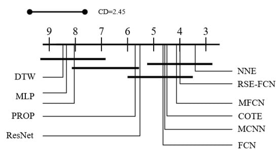
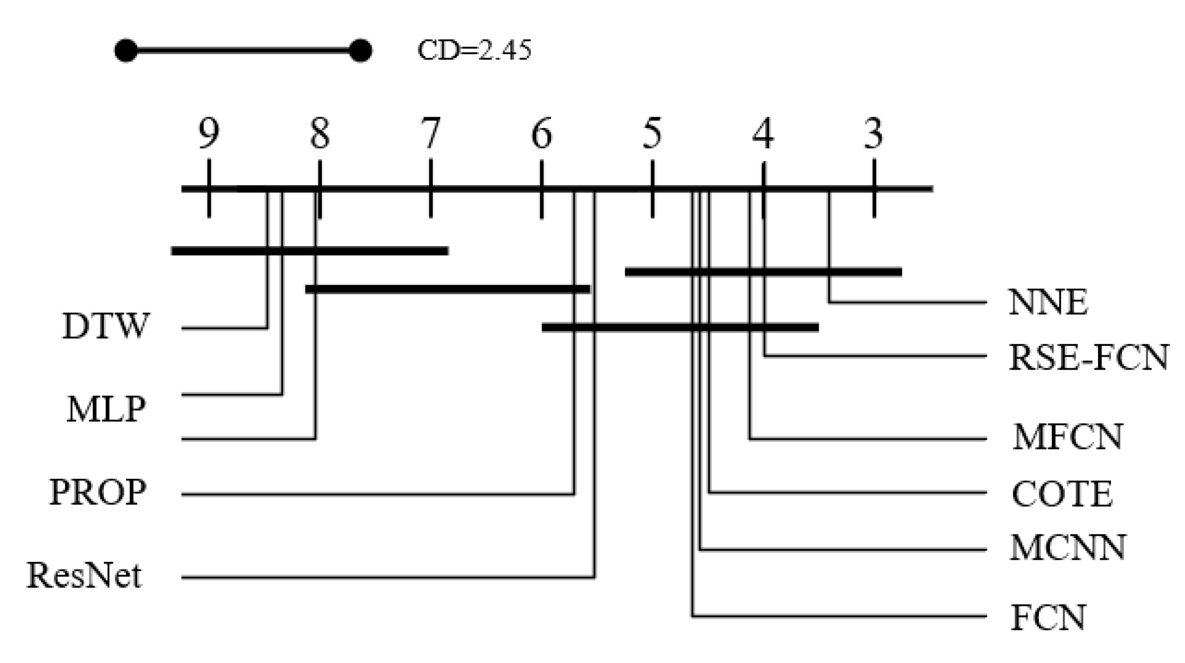
Figure 4.
Critical difference diagram of models involved in comparison.
Observation shows that RSE-FCN is in the leading position among all models within comparison. Its performance is slightly better than NNE, the 60 deep learning classifier ensembles, and much better than FCN, COTE and all the other methods. Figure 4 shows most ensemble learning methods and deep learning methods are in the first level and they have no significant difference. However, RES-FCN ranks high in this group of methods, and exceeds the competitors in other specific metrics, and it is on a par with NNE. Through further comparative analysis, it can be concluded that:
- -
- According to the three metrics in Table 1, the proposed lightweight RSE-FCN consisted within 10 FCN is at the same level as NNE which constructed by 60 neural networks, even if excluding the judgment accident of NNE on dataset DiaSizeRed (Then, the average accuracy of NNE on 25 datasets will be approximately 0.892). Furthermore, if take that dataset into consideration, RES-FCN has an obvious advantage over NNE in accuracy and robustness. This is because the superior individual FCN employed in our method establishes more accurate results than that in NNE, and it has stable performance. The ensemble built by them makes further breakthrough from this basis.
- -
- RSE-FCN outperforms three single modal neural networks and multimodal neural networks MCNN and MFCN. This illustrates building neural network ensembles by RSM manner is an effective way to solve TSC problem. RSM offers various combinations as input and thus trains many FCN classifiers which focus on different features. Compared with the multimodal neural networks like MCNN and MFCN, RSE-FCN can integrate more comprehensive information, so it is no wonder that overwhelming performance can be achieved. RSE-FCN is also more competitive than the notable non-deep-learning ensemble model COTE, showing the advantage of employing powerful deep learning method as individuals.
- -
- RSE-FCN achieves higher accuracy and more winning times than COTE and EnRS. XG-SF gives more top result than RSE-FCN but has less average accuracy, which also means it is not as robust as RSE-FCN. The three ones are methods which learn Shapelets information. Consequently, it suggests our method makes use of discriminative local information successfully, as well. Although simple and rough the converting process is, it retains the key subsequences and eliminates the information weakly related to TSC task.
After witnessing the experimental results, we briefly analyze the running time of the model. It should be note that currently in the TSC field, in order to make fair comparisons, FCN will be trained for 2000 times conventionally, since Wangs did so in the initial experiment. For other deep learning models, a fixed number of training periods are kept as well. We assume that NNE also follow this default rule. In our RSE-FCN, the feature picking and basic model training process of RSE-FCN is approximately equivalent to totally construct eight FCNs. In FCN, only a single model needs to be trained, while NNE integrated 60 models. According to the volume of these models, within the same hardware condition, the time consumption of RSE-FCN is about 6–10 times of that of single FCN, and will be 1/6–1/10 of that of NNE.
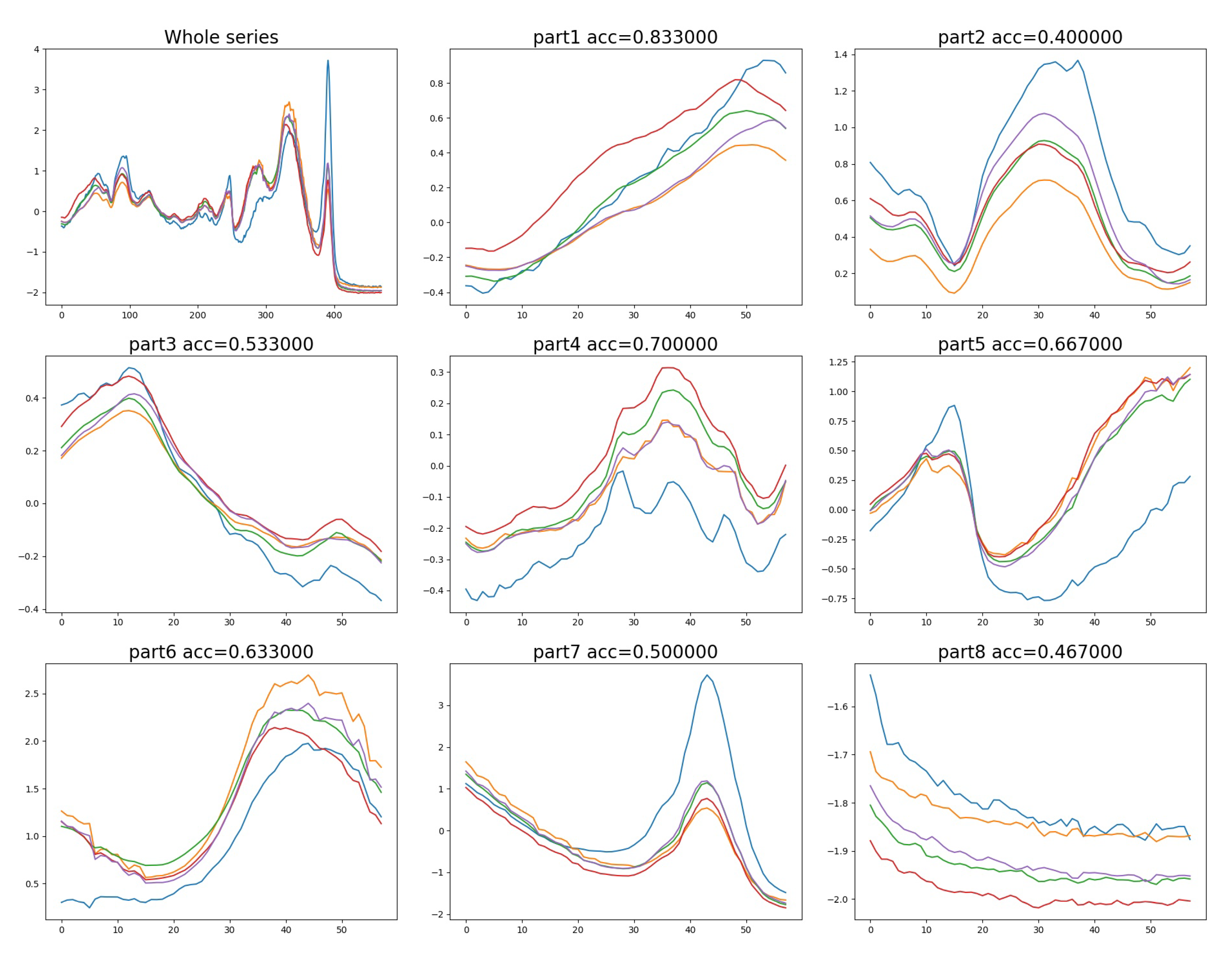
Above comparison establish the significance of our proposed RSE-FCN. Furthermore, its mechanism is analyzed by the representative dataset Beef with balanced class and middle-level time steps. Instances in Beef have dimensionality of 470 and categories of 5. Taking N = 8 as an example, as given in Figure 5, the first image in the upper left corner is the complete curve of the five categories instances. Images from 2 to 9 show the 8 equally divided intervals and their evaluating accuracy.
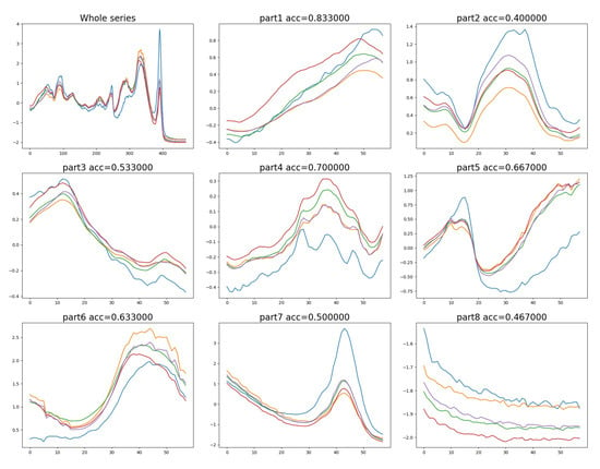
Figure 5.
Curves of time series instances of Beef dataset and the corresponding accuracy given by candidates evaluation model.
It can be seen from Figure 5 that in the second, seventh and eighth intervals, all curves mainly differ in amplitude. Furthermore, though there exists some fluctuations, compared with that in the others, they are tiny and irregular, which may be caused by noise and not category-related. Thus, in these intervals, all instances produce similar activation values when perform convolution operations with the filter matrix, making themselves to be indistinguishable, while in the rest intervals, differences appear in aspects of amplitude, change tendency, fluctuations, etc., thus they can be distinguished more easily and achieve higher accuracies. During the converting procedure of RSE-FCN, some intervals with weak discriminative feature will be discarded, so that all the random combinations will involve key information and FCNs trained by them will give fine judgment. Actually, on this dataset, some individual models which receive the discriminative local information generated by RSM did achieve higher accuracies than that based on whole series. This result proves our application of time series is reasonable and provides certain interpretability for the success of RSE-FCN.
4. Conclusions
Deep-learning-based methods show impressive performance for TSC task. However, few studies pay attention to building neural network ensembles, and the only existing NNE are not cost-effective. This paper proposes a method called RSE-FCN using Random Subspace Method to integrate the simple but outstanding FCN. It combines the strengths of learning key local information, employing superior classifier FCN and bringing promotion by ensemble. Firstly, time series are equally divided into subsequences and the top-K discriminative ones can be obtained via evaluating and screening. In that process, the main features of raw time series retain when its dimension are reduced. Then, individual models are generated with RSM deploying on the reversed subsequences and FCN serving as classifier. Finally, ensembles can be built by voting.
In experiments on UCR datasets, the lightweight RSE-FCN within 10 individuals shows same competitive with the heavy NNE, outperforming the other benchmarks. The well-trained FCNs establish a superior performance basis, the ensemble purely built by them makes further breakthrough, thus promising results can be achieved. Further analysis indicate that our usage of time series can indeed retain discriminative feature and eliminate the less relevant information, which contributes to generating strong individual classifiers. Furthermore, Random Subspace Method remains an effective manner to build good ensemble by deploying on time series subsequences.
Author Contributions
Y.Z. and C.M. came up with the creation and methodology of the models, provided the design of experiment and wrote the initial draft; J.M. participated in the programming phase and the analysis of the experimental data; L.Z. supervised the research activity planning and execution and was also responsible for ensuring that the descriptions are accurate and agreed upon by all authors. All authors have read and agreed to the published version of the manuscript.
Funding
This research received no external funding.
Acknowledgments
This work is supported by National Science Foundation of China under Grants 61871013, 71671009, 61906030, Consulting Project of China Academy of Engineering 2021XY39, the Fundamental Research Funds for the Central Universities DUT20RC(4)009 and the Natural Science Foundation of Liaoning Province 2020-BS-063.
Conflicts of Interest
The authors declare no conflict of interest.
References
- Bagnall, A.J.; Lines, J.; Bostrom, A.; Large, J.; Keogh, E.J. The great time series classification bake off: A review and experimental evaluation of recent algorithmic advances. Data Min. Knowl. Discov. 2017, 31, 606–660. [Google Scholar] [CrossRef] [PubMed] [Green Version]
- Yang, Q.; Wu, X. 10 Challenging Problems in Data Mining Research. Int. J. Inf. Technol. Decis. Mak. 2006, 5, 597–604. [Google Scholar] [CrossRef] [Green Version]
- Abanda, A.; Mori, U.; Lozano, J.A. A review on distance based time series classification. Data Min. Knowl. Discov. 2019, 33, 378–412. [Google Scholar] [CrossRef] [Green Version]
- Fawaz, H.I.; Forestier, G.; Weber, J.; Idoumghar, L.; Muller, P. Deep learning for time series classification: A review. Data Min. Knowl. Discov. 2019, 33, 917–963. [Google Scholar] [CrossRef] [Green Version]
- Wang, Z.; Yan, W.; Oates, T. Time series classification from scratch with deep neural networks: A strong baseline. In Proceedings of the 2017 International Joint Conference on Neural Networks, IJCNN 2017, Anchorage, AK, USA, 14–19 May 2017; IEEE: Piscataway, NJ, USA, 2017; pp. 1578–1585. [Google Scholar] [CrossRef] [Green Version]
- Fawaz, H.I.; Forestier, G.; Weber, J.; Idoumghar, L.; Muller, P. Transfer learning for time series classification. In Proceedings of the IEEE International Conference on Big Data, Big Data 2018, Seattle, WA, USA, 10–13 December 2018; IEEE: Piscataway, NJ, USA, 2018; pp. 1367–1376. [Google Scholar] [CrossRef] [Green Version]
- Karim, F.; Majumdar, S.; Darabi, H.; Chen, S. LSTM Fully Convolutional Networks for Time Series Classification. IEEE Access 2018, 6, 1662–1669. [Google Scholar] [CrossRef]
- Elsayed, N.; Maida, A.S.; Bayoumi, M.A. Gated Recurrent Neural Networks Empirical Utilization for Time Series Classification. In Proceedings of the 2019 International Conference on Internet of Things (iThings) and IEEE Green Computing and Communications (GreenCom) and IEEE Cyber, Physical and Social Computing (CPSCom) and IEEE Smart Data (SmartData), iThings/GreenCom/CPSCom/SmartData 2019, Atlanta, GA, USA, 14–17 July 2019; IEEE: Piscataway, NJ, USA, 2019; pp. 1207–1210. [Google Scholar] [CrossRef]
- Ma, Q.; Shen, L.; Chen, W.; Wang, J.; Wei, J.; Yu, Z. Functional echo state network for time series classification. Inf. Sci. 2016, 373, 1–20. [Google Scholar] [CrossRef]
- Zhou, W.; Hao, K.; Tang, X.; Xiao, Y.; Wang, T. Time Series Classification Based on FCN Multi-scale Feature Eensemble Learning. In Proceedings of the 2019 IEEE 8th Data Driven Control and Learning Systems Conference (DDCLS), Dali, China, 24–27 May 2019; pp. 901–906. [Google Scholar] [CrossRef]
- Bagnall, A.J.; Lines, J.; Hills, J.; Bostrom, A. Time-series classification with COTE: The collective of transformation-based ensembles. In Proceedings of the 32nd IEEE International Conference on Data Engineering, ICDE 2016, Helsinki, Finland, 16–20 May 2016; pp. 1548–1549. [Google Scholar] [CrossRef]
- Lines, J.; Bagnall, A.J. Time series classification with ensembles of elastic distance measures. Data Min. Knowl. Discov. 2015, 29, 565–592. [Google Scholar] [CrossRef]
- Ji, C.; Zou, X.; Hu, Y.; Liu, S.; Lyu, L.; Zheng, X. XG-SF: An XGBoost Classifier Based on Shapelet Features for Time Series Classification. In Proceedings of the 2018 International Conference on Identification, Information and Knowledge in the Internet of Things, IIKI 2018, Beijing, China, 19–21 October 2018; Elsevier: Amsterdam, The Netherlands, 2018; Volume 147, pp. 24–28. [Google Scholar] [CrossRef]
- Raza, A.; Kramer, S. Ensembles of Randomized Time Series Shapelets Provide Improved Accuracy while Reducing Computational Costs. arXiv 2017, arXiv:1702.06712. [Google Scholar]
- Fawaz, H.I.; Forestier, G.; Weber, J.; Idoumghar, L.; Muller, P. Deep Neural Network Ensembles for Time Series Classification. arXiv 2019, arXiv:1903.06602. [Google Scholar]
- Zhao, B.; Lu, H.; Chen, S.; Liu, J.; Wu, D. Convolutional neural networks for time series classification. J. Syst. Eng. Electron. 2017, 28, 162–169. [Google Scholar] [CrossRef]
- Zheng, Y.; Liu, Q.; Chen, E.; Ge, Y.; Zhao, J.L. Time Series Classification Using Multi-Channels Deep Convolutional Neural Networks. In Web-Age Information Management, Proceedings of the 15th International Conference, WAIM 2014, Macau, China, 16–18 June 2014; Lecture Notes in Computer Science; Springer: Amsterdam, The Netherlands, 2014; Volume 8485, pp. 298–310. [Google Scholar] [CrossRef]
- Ho, T.K. The Random Subspace Method for Constructing Decision Forests. IEEE Trans. Pattern Anal. Mach. Intell. 1998, 20, 832–844. [Google Scholar] [CrossRef] [Green Version]
- Kotsiantis, S.B. A random subspace method that uses different instead of similar models for regression and classification problems. Int. J. Inf. Decis. Sci. 2011, 3, 173–188. [Google Scholar] [CrossRef]
- Wang, G.; Zhang, Z.; Sun, J.; Yang, S.; Larson, C.A. POS-RS: A Random Subspace method for sentiment classification based on part-of-speech analysis. Inf. Process. Manag. 2015, 51, 458–479. [Google Scholar] [CrossRef]
- Ye, L.; Keogh, E.J. Time series shapelets: A new primitive for data mining. In Proceedings of the 15th ACM SIGKDD International Conference on Knowledge Discovery and Data Mining, Paris, France, 28 June–1 July 2009; IV, J.F.E., Fogelman-Soulié, F., Flach, P.A., Zaki, M.J., Eds.; ACM: New York, NY, USA, 2009; pp. 947–956. [Google Scholar] [CrossRef]
- Hills, J.; Lines, J.; Baranauskas, E.; Mapp, J.; Bagnall, A.J. Classification of time series by shapelet transformation. Data Min. Knowl. Discov. 2014, 28, 851–881. [Google Scholar] [CrossRef] [Green Version]
- Mueen, A.; Keogh, E.J.; Young, N.E. Logical-shapelets: An expressive primitive for time series classification. In Proceedings of the 17th ACM SIGKDD International Conference on Knowledge Discovery and Data Mining, San Diego, CA, USA, 21–24 August 2011; Apté, C., Ghosh, J., Smyth, P., Eds.; ACM: New York, NY, USA, 2011; pp. 1154–1162. [Google Scholar] [CrossRef]
- Dau, H.A.; Bagnall, A.J.; Kamgar, K.; Yeh, C.M.; Zhu, Y.; Gharghabi, S.; Ratanamahatana, C.A.; Keogh, E.J. The UCR Time Series Archive. arXiv 2018, arXiv:1810.07758. [Google Scholar] [CrossRef]
- Cui, Z.; Chen, W.; Chen, Y. Multi-Scale Convolutional Neural Networks for Time Series Classification. arXiv 2016, arXiv:1603.06995. [Google Scholar]
- Rakthanmanon, T.; Campana, B.J.L.; Mueen, A.; Batista, G.E.A.P.A.; Westover, M.B.; Zhu, Q.; Zakaria, J.; Keogh, E.J. Searching and mining trillions of time series subsequences under dynamic time warping. In Proceedings of the The 18th ACM SIGKDD International Conference on Knowledge Discovery and Data Mining, KDD ’12, Beijing, China, 12–16 August 2012; Yang, Q., Agarwal, D., Pei, J., Eds.; ACM: New York, NY, USA, 2012; pp. 262–270. [Google Scholar] [CrossRef] [Green Version]
- Demsar, J. Statistical Comparisons of Classifiers over Multiple Data Sets. J. Mach. Learn. Res. 2006, 7, 1–30. [Google Scholar]
Publisher’s Note: MDPI stays neutral with regard to jurisdictional claims in published maps and institutional affiliations. |
© 2021 by the authors. Licensee MDPI, Basel, Switzerland. This article is an open access article distributed under the terms and conditions of the Creative Commons Attribution (CC BY) license (https://creativecommons.org/licenses/by/4.0/).