Quantitative Description for Sand Void Fabric with the Principle of Stereology

Abstract

Based on the principle of stereology to describe void fabric, the fabric tensor is redefined by the idea of normalization, and a novel quantitative description method for the orthotropic fabric of granular materials is presented. The scan line is described by two independent angles in the stereo space, and the projection of the scan line on three orthogonal planes is used to determine the plane tensor. The second-order plane tensor can be described equivalently by two invariants, which describe the degree and direction of anisotropy of the material, respectively. In the three-dimensional orthogonal space, there are three measurable amplitude parameters on the three orthogonal planes. Due to the normalized definition of tensor in this paper, there are only two independent variations of the three amplitude parameters, and any two amplitude parameters can be used to derive the three-dimensional orthotropic fabric tensor. Therefore, the same orthorhombic anisotropy structure can be described by three fabrics, which enriches the theoretical description of orthotropy greatly. As the geometric relationship of the stereoscopic space scan line changes, the three sets of orthotropic fabrics degenerate into different forms of transversely isotropic and isotropic fabrics naturally and have a clear physical meaning. The novel fabric tensor is quantitatively determined based on mathematical probability and statistics. The discrete distribution of voids in space is projected as a scalar measurable parameter on a plane. This parameter is related to the macroscopic constitutive relationship directly and can be used to describe the effect of microscopic voids on the macroscopic phenomenon of materials.

1. Introduction

The void ratio is one of the most important, earliest, and most widely used material parameters for controlling the mechanical response of the soil. In critical state soil mechanics, it is the only material physical parameter that describes the critical state. However, Li and Dafalias [1], Zhao and Guo [2] and Abouzar et al. [3] have recently confirmed that the critical state of soil was not unique due to the existence of fabric anisotropy, i.e., the relationship between the void ratio of critical state and hydrostatic pressure was not unique, which was a challenge to the uniqueness hypothesis for the critical state theory of soil mechanics. According to the anisotropic characteristics of soil meso-structure, Chow et al. [4] studied the meso-structure of particles under one-dimensional consolidation conditions and found that the particle structure had a horizontal arrangement trend, and the void structure showed a similar orientation trend. Sun et al. [5] and Zheng et al. [6] found that the void fabric tensor and particle sphericity, relative density, and coordination number have a strong functional relationship through the image analysis of loose and dense sand specimens. Hu et al. [7] presented a fabric tensor-based bounding surface model accounting for the anisotropic behavior of granular materials. Zhang et al. [8] established the relations between the macroscopic volumetric strain, shear strain, and void fabric combined with the micromechanics theory, and linked with void fabric tensor. Zhao et al. [9] considered the effects of initial anisotropy, porosity, stress ratio, loading direction, and intermediate principal stress ratio, and established the anisotropic evolution law for fabric. Although the void fabric has a substantial impact on the mechanical properties of sand, the relative lag in the development of mesoscopic testing technology, experiment and description theory of void fabric has led to a lack of understanding of void fabric and has restricted the study of the mechanical properties by the method of macro and micro combination.

The three main causes of the meso-fabric of sand are the anisotropic distribution of contact normal particles, void space, and the arrangement of the nonspherical particles [10]. It is difficult to consider the three causes simultaneously because they have different physical and geometric meanings and applications. Therefore, the different fabric theories and their description methods have been formed. For example, Oda [10] and Tobita [11] defined the fabric tensor by considering the arrangement direction of the long axes of sand particles and the distribution of contact stress, which laid the foundation of the fabric theory and has been widely applied. However, the determination of single-particle direction and the direction of contact normal between particles has always puzzled scholars, who believed that these two factors were hardly measured accurately [12,13]. Thus, there are more qualitative studies than quantitative studies for fabric, which is the biggest obstacle to be applied to soil constitutive relationships. In the author’s work of establishing strength criterion [14], constitutive model [15] and potential theory [16] with fabric to describe anisotropy, the fabric description has always been at the core of thinking. Comparatively speaking, the description of void in three kinds of fabric is more intuitive and easier to accept, but the bottleneck is the development of its theory and measurement technology. Void fabric is a mathematical relationship describing the spatial distribution of voids in soil and there are three main theories to describe void fabric. First, Oda [17] proposed the 2D void fabric theory and its measurement method; then Bhatia and Soliman [18] used it in an experimental study. This method was difficult to popularize because it involved segmentation and image recognition, such as the center of gravity, boundary, shape, arrangement, and movement of particles. Second, Bagi [19] proposed a dual geometric system to describe the effects of particles and voids; however, the difficulty in defining the 3D void space was its application. Based on Bagi’s study [19], Li and Li [20] modified the theoretical expression of fabric. Using the modified expression, Fu and Dafalias [21] obtained 2D linear relationships of a different fabric caused by discrete element simulation. Nevertheless, there were still similar problems in the quantitative determination of Oda’s fabrics [17]. Third, the void fabric was determined by the stereology theory. Hilliard [22] first established the mathematical framework and determined the void distribution in different planes and spaces with scan lines quantitatively. Later, Kanatani [23,24,25] extended the Hilliard method to the form of Cartesian coordinate tensor, and for the first time unified the Hilliard method to solve different problems into a unique mathematical framework. Buffon transformed and derived the inverse transform of Buffon transform that determined the fabric tensor with the scan line directly. Based on the work of Kanatani [23,24,25], Kuo et al. [26] and Shiva et al. [27] conducted quantitative detection of the void tensor for sand. Ghedia et al. [28] and Theocharis et al. [29] used scan lines to quantify the void in granular materials. The results showed that the method can quantify the anisotropy and 3D evolution of void fabric adequately. Through DEM analysis, it was found that the method was adapted to the existing quantification methods of the void fabric. All the above studies show the rationality of using scan lines to quantify the void of granular materials, but there are relatively few theoretical and experimental results. To sum up, the third theoretical basis is dependable, and the test analysis is simple.

According to the theoretical description of the particle arrangement fabric and the quantitative detection of the plane amplitude parameters, authors [30,31] presented a quantitative detection method of the plane parameters for the sand void fabric by stereology [32]. Based on this method, there was also a better effect on the quantitative determination of rock fracture fabrics [33,34]. Hence, for the shortcomings of the existing void fabric theory in the measurement process, the authors redefined the theoretical expression of the void fabric. On the basis of plane quantitative measurement for void fabric, the method was extended to 3D space, and theoretical expressions of void fabric for different 3D fabric were derived by using quantitative measurement parameters on three orthogonal planes, i.e., the 3D fabric expressions of orthotropic and transversely isotropic. In this paper, the physical and geometric significance was analyzed in detail to popularize and apply quantitative determination technology of void fabric.

2. Existing Theories of the Void Fabric Tensors

The distribution equation of void space is determined based on the principle of stereology. The equation is determined by the average porosity (scalar) and the symmetric fabric tensor that trace is 0 [35]. Tobita [35] used the REV (Representative Element Volume) method to detect the void fabric distribution quantitatively. As shown in Figure 1, the first step is to select a sample space with enough particles to perform mathematical statistics. The second step is to determine a measurement sphere. Finally, the length L in the sphere is the scan line, and the length of the scan line truncated by the void is the measured void length. By rotating the scan line throughout the sphere, the void distribution in the sphere is measured. Therefore, the void distribution in spherical coordinates is l_l(α,β) = ∑l_i(α,β), and the ratio of scan lines to void is as follows:

$$L_{\mathrm{L}}(\alpha ,\beta )=\frac{l_l(\alpha ,\beta )}{L}=\frac{l_l(\alpha ,\beta )}{2R}$$

(1)

where L_L(α, β) is the porosity of the scan line. L is the length of the scan line. R is the radius. α and β are independent integral variables of the integral interval.

Then, the average porosity in a unit sphere is as follows:

$$n_m=\frac{1}{4\pi }{\displaystyle {\int }_0^{2\pi }{\displaystyle {\int }_0^{\pi }{L}_{\mathrm{L}}(\alpha ,\beta )}}\sin \alpha \mathrm{d}\alpha \mathrm{d}\beta$$

(2)

where n_m is the average porosity per unit measured through the m-th scan line. Equation (2) expresses in the Cartesian coordinate system as follows:

$$n_m=\frac{{\displaystyle \int {\displaystyle {\int }_{Syz}{l}_x\mathrm{d}y\mathrm{d}z}}+{\displaystyle \int {\displaystyle {\int }_{Szx}{l}_y\mathrm{d}z\mathrm{d}x}}+{\displaystyle \int {\displaystyle {\int }_{Sxy}{l}_z\mathrm{d}x\mathrm{d}y}}}{8\pi }$$

(3)

where l_x, l_y, and l_z are the distribution functions of the void density on the corresponding coordinate plane, respectively. s_yz, s_zx, and s_xy are the integral intervals on the corresponding plane, respectively.

The void distribution equation is expressed as average porosity and a symmetric fabric tensor that’s trace is 0 [23,24,25] and reads:

$$N(\overrightarrow{n})=n_m(1+N_{ij}{n}_i{n}_j+N_{ijkl}{n}_i{n}_j{n}_k{n}_l+\cdots )$$

(4)

where $N\left(\overrightarrow{n}\right)$ is the average void distribution function, $\overrightarrow{n}$ is the unit vector, $N_{i_1{i}_2\dots i_n}$ is a void tensor that’s trace is 0 and is reads:

$$N_{i_1{i}_2\dots i_n}=\frac{2n+1}{2^n}\left(\begin{array}{c}2n\\ n\end{array}\right){\mathsf{\Omega }}_{i_1{i}_2\dots i_n}$$

(5)

where ${\mathsf{\Omega }}_{i_1{i}_2\dots i_n}$ is the tensor defined by Kanatani [23,24,25] and reads:

$${\mathsf{\Omega }}_{i_1{i}_2\dots i_n}=\frac{1}{4\pi n_m}{\displaystyle {\int }_{\mathsf{\Omega }}{n}_{i_1{i}_2\dots i_n}{n}_{in}{L}_{\mathrm{L}}(\alpha ,\beta )}\mathrm{d}\overrightarrow{n}$$

(6)

The key of Equation (4) to describe the void distribution is how to measure n_m and $N_{i_1{i}_2\dots i_n}$.

3. Novel Void Fabric Tensors Definitions

Based on the description theory of void tensors in the principle of stereology and the theoretical research results of existing void tensors, a novel test method for fabric tensor is presented in this paper.

3.1. Definition of Void Fabric

The void fabric describes the distribution form of the three orthogonal planes where the value of trace is equal to 1. Thus, according to the characteristic and combining with normalized ideas, the equation of the void fabric tensor is defined and reads:

$$M_{i_1{i}_2\dots i_n}=\frac{{\displaystyle {\int }_{\mathsf{\Omega }}{n}_{i_1{i}_2\dots i_n}{n}_{in}{L}_{\mathrm{L}}(\alpha ,\beta )}\mathrm{d}\overrightarrow{n}}{{\displaystyle {\int }_{\mathsf{\Omega }}{L}_{\mathrm{L}}(\alpha ,\beta )}\mathrm{d}\overrightarrow{n}}$$

(7)

where $M_{i_1{i}_2\dots i_n}$ is the void fabric tensor, which is used for the microscopic quantitative detection of the void tensor directly.

The tensor determined by Equation (7) accurately describes the variation of void space distribution in theory. However, in practice, the second-order fabric tensor has been able to describe the variation of void distribution. Hence, the influence of higher-order tensors is ignored. Equation (7) describes the second-order tensor as follows.

$$M_{ij}=\frac{{\displaystyle \int L_{\mathrm{L}}({\alpha }_m,{\beta }_m)n_i{n}_j\mathrm{d}\overrightarrow{n}}}{{\displaystyle \int L_{\mathrm{L}}({\alpha }_m,{\beta }_m)\mathrm{d}\overrightarrow{n}}}$$

(8)

where M_ij is the second-order symmetric fabric tensor. α_m and β_m are the description angles of the m-th scan line. n_in_j is the direction component of the second-order fabric tensor.

According to Equation (5), a tensor that’s trace is 0 is obtained directly and reads:

$$N_{ij}=\frac{15}{2}(M_{ij}-\frac{1}{3}{\delta }_{ij})$$

(9)

where N_ij is the symmetric fabric tensor that’s trace is 0 describing the void distribution. δ_ij is the Kronecker tensor.

According to Equation (4), the void distribution equation of the second-order tensor is as follows.

$$N(\overrightarrow{n})=n_m(1+N_{ij}{n}_i{n}_j)$$

(10)

where n_m is the form described by Equation (2).

From Equation (8), the description method in this paper improved the fabric definition. According to the definition of measurement voids, the measurement process is expressed as the following equation by series.

$$M_{ij}=\frac{{\displaystyle \sum _{m=0}^{N-1}\frac{L_{\mathrm{L}}({\alpha }_m,{\beta }_m)n_i{n}_j}{N}}}{{\displaystyle \sum _{m=0}^{N-1}\frac{L_{\mathrm{L}}({\alpha }_m,{\beta }_m)}{N}}}=\frac{{\displaystyle \sum _{m=0}^{N-1}{L}_{\mathrm{L}}({\alpha }_m,{\beta }_m)n_i{n}_j}}{{\displaystyle \sum _{m=0}^{N-1}{L}_{\mathrm{L}}({\alpha }_m,{\beta }_m)}}$$

(11)

From Figure 2, the components of the unit vector $\overrightarrow{n}$ in the three orthogonal directions are $n_1=\cos \alpha$, $n_2=\sin \alpha \sin \beta$, and $n_3=\sin \alpha \cos \beta$, i.e., the tensor defined by Equation (11) is the following equation.

$$M_{ij}=\left[\begin{array}{ccc}{M}_{11}& M_{12}& M_{13}\\ M_{21}& M_{22}& M_{23}\\ M_{31}& M_{32}& M_{33}\end{array}\right]$$

(12)

From Equations (11) and (12), the trace of the novel void tensor M_ij is equal to 1, so the trace of the tensor described in Equation (9) is equal to 0, which provides great convenience for the derivation of the void distribution equation and the determination of the test tensor.

3.2. A Novel Definition of 2D Void Fabric

As shown in the unit test sphere in Figure 1, the spatial distribution of voids cannot be obtained directly by spatial scan line but can be obtained by plane image analysis of void distribution and then can be carried out reasonably in 3D modeling. The void projection distribution on three orthogonal planes is obtained by plane image analysis, and the detailed quantitative method is shown in the reference [35]. Then the void projection described in Figure 1 on the three orthogonal planes is measured by the actual image, i.e., the fabric tensor on the three orthogonal planes x₁-x₃, x₁-x₂, and x₂-x₃. According to Equation (12), the tensor on the plane x₁-x₃ is the following equation.

$$M_{ij}^{1-3}=\left[\begin{array}{cc}{M}_{11}& M_{13}\\ M_{31}& M_{33}\end{array}\right]$$

(13)

From Equation (11), N_ij is the partial tensor of M_ij, then $N_{ij}^{1-3}$ is described equivalently by the second invariant and component angle of $M_{ij}^{1-3}$, and reads:

$$\begin{array}{l}{b}_1=\sqrt{J_2}=\begin{array}{c}\sqrt{{\left[\frac{{\displaystyle \sum _{m=0}^{N-1}{L}_{\mathrm{L}}({\alpha }_m,{\beta }_m)\left({\cos }^2{\alpha }_m-{\sin }^2{\alpha }_m{\cos }^2{\beta }_m\right)}}{{\displaystyle \sum _{m=0}^{N-1}{L}_{\mathrm{L}}({\alpha }_m,{\beta }_m)}}\right]}^2+{\left(\frac{{\displaystyle \sum _{m=0}^{N-1}{L}_{\mathrm{L}}({\alpha }_m,{\beta }_m)\sin 2{\alpha }_m\cos {\beta }_m}}{{\displaystyle \sum _{m=0}^{N-1}{L}_{\mathrm{L}}({\alpha }_m,{\beta }_m)}}\right)}^2}\end{array}\\ {\theta }_1=\frac{1}{2}\arctan \frac{2M_{13}}{M_{11}-M_{33}}\end{array}\}$$

(14)

where b₁ is the void amplitude parameter and is the second invariant of the void tensor in plane x₁-x₃, which is a scalar and describes the anisotropic degree. θ₁ is the angle between the major direction of the void fabric and the direction of the coordinate axis, which describes the plane direction of the void fabric anisotropic degree.

Similarly, the invariants and directions in the planes x₁-x₂ and x₂-x₃ are the following equations.

$$\begin{array}{l}{b}_2=\sqrt{J_2}=\begin{array}{c}\sqrt{{\left[\frac{{\displaystyle \sum _{m=0}^{N-1}{L}_{\mathrm{L}}({\alpha }_m,{\beta }_m)\left({\cos }^2{\alpha }_m-{\sin }^2{\alpha }_m{\sin }^2{\beta }_m\right)}}{{\displaystyle \sum _{m=0}^{N-1}{L}_{\mathrm{L}}({\alpha }_m,{\beta }_m)}}\right]}^2+{\left(\frac{{\displaystyle \sum _{m=0}^{N-1}{L}_{\mathrm{L}}({\alpha }_m,{\beta }_m)\sin 2{\alpha }_m\sin {\beta }_m}}{{\displaystyle \sum _{m=0}^{N-1}{L}_{\mathrm{L}}({\alpha }_m,{\beta }_m)}}\right)}^2}\end{array}\\ {\theta }_2=\frac{1}{2}\arctan \frac{2M_{12}}{M_{11}-M_{22}}\end{array}\}$$

(15)

$$\begin{array}{l}{b}_3=\sqrt{J_2}=\begin{array}{c}\sqrt{{\left[\frac{{\displaystyle \sum _{m=0}^{N-1}{L}_{\mathrm{L}}({\alpha }_m,{\beta }_m){\sin }^2{\alpha }_m\cos 2{\beta }_m}}{{\displaystyle \sum _{m=0}^{N-1}{L}_{\mathrm{L}}({\alpha }_m,{\beta }_m)}}\right]}^2+{\left(\frac{{\displaystyle \sum _{m=0}^{N-1}{L}_{\mathrm{L}}({\alpha }_m,{\beta }_m){\sin }^2{\alpha }_m\sin 2{\beta }_m}}{{\displaystyle \sum _{m=0}^{N-1}{L}_{\mathrm{L}}({\alpha }_m,{\beta }_m)}}\right)}^2}\end{array}\\ {\theta }_3=\frac{1}{2}\arctan \frac{2M_{23}}{M_{22}-M_{33}}\end{array}\}$$

(16)

where b₂ and b₃ are the void amplitude parameters on planes of x₁-x₂ and x₂-x₃, which describes the anisotropic degree. θ₂ and θ₃ are the angles of the two corresponding planes.

According to Equation (12), the distribution of the void tensor on three orthogonal planes is described by its invariant.

$$N_i(n_m^{2D},{\theta }_m)=n_m^{2D}(1+b_i\cos 2({\theta }_m-{\theta }_i))$$

(17)

where θ_m is the angle of the unit vector in the plane coordinate system. $n_m^{2D}$ is the average porosity of the plane, which is determined directly by image analysis. b_i (i = 1,2,3) are the void amplitude parameters defined in Equations (14)–(16), respectively. θ_i (i = 1,2,3) are the angle invariants defined by the corresponding equation. Due to M_kk = 1, the values of all three amplitude parameters are between 0 and 1. When b_i = 0, the voids are distributed evenly and the specimen is isotropic. When b_i = 1, the voids are distributed ideally in a fixed direction. θ_i represents the anisotropic direction of the void distribution.

4. Novel Void Fabric Tensors Definitions

According to the novel fabric definition of the normalized ideas, i.e., M_kk = 1, there are only two independent variables in the amplitude parameters of b₁, b₂, and b₃. Hence, as long as the amplitude parameters on any two orthogonal planes are measured in theory, the fabric tensor is determined uniquely. Then it is deduced that any two amplitude parameters are used to describe the void fabric tensor.

4.1. Orthotropic Void Fabrics

The void amplitude parameter (b₁, b₂ and b₃) obtained by Equations (14)–(16) in 2D space is not equal to the principal value (M₁, M₂ and M₃) in 3D space, but proportional to it. Therefore, the following void fabric equation is established and reads:

$$M_{ij}=\left[\begin{array}{ccc}{M}_1& 0& 0\\ 0& M_2& 0\\ 0& 0& M_3\end{array}\right]$$

(18)

According to M_kk = 1 and any two parameters from b₁, b₂, and b₃, the orthotropic fabric tensor is obtained, and the detailed derivative process is shown in reference [31]. The three equations of orthotropic fabric tensor are as follows:

$$\begin{array}{l}{M}_1=\frac{(1+b_1)(1+b_2)}{3+b_1+b_2-b_1{b}_2}\\ M_2=\frac{(1+b_1)(1-b_2)}{3+b_1+b_2-b_1{b}_2}\\ M_3=\frac{(1-b_1)(1+b_2)}{3+b_1+b_2-b_1{b}_2}\end{array}\}$$

(19)

$$\begin{array}{l}{M}_1=\frac{(1+b_1)(1-b_3)}{3-b_1-b_3-b_1{b}_3}\\ M_2=\frac{(1-b_1)(1+b_3)}{3-b_1-b_3-b_1{b}_3}\\ M_3=\frac{(1-b_1)(1-b_3)}{3-b_1-b_3-b_1{b}_3}\end{array}\}$$

(20)

$$\begin{array}{l}{M}_1=\frac{(1+b_2)(1+b_3)}{3-b_2+b_3+b_2{b}_3}\\ M_2=\frac{(1-b_2)(1+b_3)}{3-b_2+b_3+b_2{b}_3}\\ M_3=\frac{(1+b_2)(1-b_3)}{3-b_2+b_3+b_2{b}_3}\end{array}\}$$

(21)

Equation (19) is the three principal value parameters M₁, M₂ and M₃ of the orthotropic void fabric tensor, which are calculated by the void amplitude parameters b₁ and b₂ of the surface x₁-x₃ and surface x₁-x₂. Similarly, Equation (20) is the three principal value parameters M₁, M₂ and M₃ of the orthotropic void fabric tensor, which are calculated by the void amplitude parameters b₁ and b₃ of the surface x₁-x₃ and surface x₂-x₃. Equation (21) is the three principal value parameters M₁, M₂ and M₃ of the orthotropic void fabric tensor, which are calculated by the void amplitude parameters b₂ and b₃ of the surface x₁-x₂ and surface x₂-x₃.

Therefore, as long as any two void invariants of the three orthogonal planes are obtained through experiments, the orthogonal anisotropic fabric is determined by Equation (18). Equations (19)–(21) not only provided more options for the theoretical description of M_ij but also provided more flexible methods for the orthotropic experimental measurement of void fabric for sand.

4.2. Transversely Isotropic Void Fabrics

In this paper, the definition of orthotropic void fabric is based on the measurement method of stereology, which describes the orthotropic distribution of voids. When the scan line distribution meets certain geometric conditions, it is simplified into the form of transversely isotropy and isotropy naturally.

In Equations (14) and (15), when β_m = π/4, then b₁ = b₂, i.e., the void parameters in the two directions are equal. At this point, the material shows as transversely isotropic, and Equation (19) is simplified into 3D fabric and reads:

$$M_{ij}=\frac{1}{3-b}\left[\begin{array}{ccc}1+b& 0& 0\\ 0& 1-b& 0\\ 0& 0& 1-b\end{array}\right]$$

(22)

where:

$$b=\sqrt{{\left[\frac{{\displaystyle \sum _{m=0}^{N-1}{L}_{{}_{\mathrm{L}}}({\alpha }_m,{\beta }_m)({\cos }^2{\alpha }_m-\frac{1}{2}{\sin }^2{\alpha }_m)}}{{\displaystyle \sum _{m=0}^{N-1}{L}_{\mathrm{L}}({\alpha }_m,{\beta }_m)}}\right]}^2+\frac{1}{2}{\left(\frac{{\displaystyle \sum _{m=0}^{N-1}{L}_{\mathrm{L}}({\alpha }_m,{\beta }_m)\sin 2{\alpha }_m}}{{\displaystyle \sum _{m=0}^{N-1}{L}_{\mathrm{L}}({\alpha }_m,{\beta }_m)}}\right)}^2}$$

(23)

where b is the amplitude parameter of the transversely isotropic void tensor, and its theoretical value range is [0,1], which is obtained by solving the invariant of the planar void fabric tensor from any one of the two homogeneous planes. b₁ = b₂ = b indicates that the void tensor invariants of the two planes are equal. Equation (22) is used to describe the transversely isotropy of the voids in the sand by an amplitude parameter. The physical geometric meaning of transversely isotropy is legible.

According to Equations (9) and (22), N_ij is obtained and reads:

$$N_{ij}=\frac{5}{3-b}\left[\begin{array}{ccc}2b& 0& 0\\ 0& -b& 0\\ 0& 0& -b\end{array}\right]$$

(24)

The average porosity n_m in Equation (9) is easy to determine. Thus, when N_ij is determined, the distribution of transversely isotropic void space is determined.

Similarly, when α_m = π/2 in Equation (14) and β_m = 0 in Equation (16), then b₁ = b₃ and Equation (20) is simplified into the form of transversely isotropy and reads:

$$M_{ij}=\frac{1}{3+b}\left[\begin{array}{ccc}1+b& 0& 0\\ 0& 1+b& 0\\ 0& 0& 1-b\end{array}\right]$$

(25)

where b is the following:

$$b=\sqrt{{\left[\frac{{\displaystyle \sum _{m=0}^{N-1}{L}_{\mathrm{L}}({\alpha }_m,{\beta }_m)\cos 2{\alpha }_m}}{{\displaystyle \sum _{m=0}^{N-1}{L}_{\mathrm{L}}({\alpha }_m,{\beta }_m)}}\right]}^2+{\left(\frac{{\displaystyle \sum _{m=0}^{N-1}{L}_{\mathrm{L}}({\alpha }_m,{\beta }_m)\sin 2{\alpha }_m}}{{\displaystyle \sum _{m=0}^{N-1}{L}_{\mathrm{L}}({\alpha }_m,{\beta }_m)}}\right)}^2}$$

(26)

where b is the parameter of transversely isotropic fabric. The variable of Equation (14) after degenerating is β_m. The variable of Equation (16) after degenerating is α_m. For convenience, the variable α_m is used here.

When β_m = π/2 in Equation (15) and α_m = 0 in Equation (16), then b₂ = b₃. Equation (19) is simplified into the following equation.

$$M_{ij}=\frac{1}{3+b^2}\left[\begin{array}{ccc}{(1+b)}^2& 0& 0\\ 0& 1-b^2& 0\\ 0& 0& {(1-b)}^2\end{array}\right]$$

(27)

where the equation of b is the same as the form of Equation (26), but the variable β_m is different. Although the amplitude parameter is simplified into a transversely isotropic form, the simplified fabric tensor (Equation (27)) is orthotropic.

To sum up, when the orthotropic void fabrics are simplified into transversely isotropy, Equation (22) is applied to the detection and application of transversely isotropy void fabric directly. Although Equation (25) has some contradictions in the degradation process, it is consistent with the description results of the existing void fabric. Hence, under certain conditions, Equation (25) still has certainly applicable scope. Equation (27) is still in the orthotropic form after degradation and cannot describe transversely isotropic materials. However, whether it is used as an amplitude parameter to describe the orthotropic properties of materials under certain simplified conditions remains to be studied.

5. Image Analysis of Void Fabric

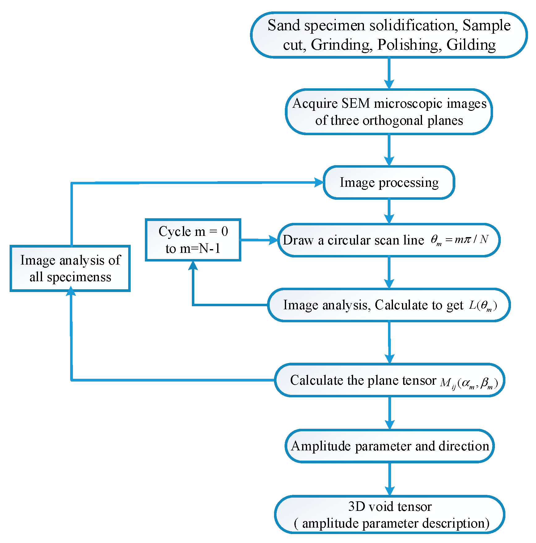
5.1. Analysis Procedure and Method

According to the theoretical determination method of void tensor presented in this paper, an image analysis program is compiled with Matlab, and the program frame diagram is presented in Figure 3, which shows the whole process of fabric determination. Since the major purpose of this study is to determine the orthotropy of the void tensor, cube specimens are required for specimen collection and preparation.

The calculation program in Figure 3 is composed of two parts. The first part is the Matlab program of image processing, which aims to reduce the interference of environmental factors and to obtain a clear binary image for image analysis. The second part is the Matlab program of image analysis, which is the most critical part of the process. To obtain the probability statistic law of the void distribution in three orthogonal directions, the program has to perform statistical analysis on the void distribution of multiple pictures from different orthogonal directions, and there are two cyclic programs to accomplish this task. Finally, the void distribution extracted by image analysis is used to calculate the void amplitude parameters, direction, and spatial distribution of the void plane.

5.2. Parallel Scan Line Analysis Method

According to the principle of stereology, the scan line is the key to the test of void fabric. The void is the sum of all pixels with a value 0 in a binary image. Porosity is the ratio of the voids to the total pixels of the scan line, this definition is different from the soil mechanics, while their spatial distribution is the same and can be interchangeable.

In the image analysis, the scan line and the image processing diagram of specimens are operated with “&”, and the intersection image of the scan line and void is obtained, then void data is extracted. Figure 4 shows the calculation results of image analysis with parallel scan lines. Figure 4a is the diagram of the scan line (60°). Figure 4b is the binary image. Figure 4c is the result measured by the 60° scan line and Figure 4d is the result measured by the 30° scan line. The number of scan lines is 180.The scan line is drawn by AutoCAD. Figure 4c,d show that the calculated image will better describe the void distribution.

Before test verification, the influence of scan line density and angle needs to be analyzed. Two examples are designed for the same image. One is to analyze the image with different scan line densities and the same angle. The other is to analyze the image with different scan lines at the same density and different angles. Figure 5 shows the influence of scan line density on test results, and the relationship between porosity and scan line density is obtained by increasing the number of scan lines with a fixed angle of the scan line. The images adopt three orthogonal planes of sand specimens from Kuo et al. [26].

As is presented in Figure 5, the fewer the number of test lines, the greater the impact on the porosity. However, as the number of scan lines increases, the fluctuation tends to be stable and nearly constant. When the number of scan lines is more than 100, the porosity fluctuation is ignored. Therefore 230 scan lines were used in this test. Figure 6 shows the relationship between the angle of parallel scan lines and porosity. The angle of the scan lines varied from 0° to 180° with an angle interval of 10°. Figure 6a shows that the porosity varies little with the angle of the scan line and is close to a constant value. Figure 6b intuitively shows that the plane porosity measured by parallel scan lines is an invariant, which cannot reflect the plane distribution of voids.

To sum up, the average porosity fluctuated greatly when the number of scan lines was small, but after reaching a certain number, the value tends to be constant. The average porosity is a scalar, which is independent of the direction. Thus, parallel scan lines can measure the average porosity, but cannot measure the distribution of voids.

5.3. Analysis Method with Annular Scan Line

To obtain the distribution of voids, an annular scan line has to be used. Figure 7a shows the drawing of the annular scan line, which is a method used by some scholars such as Kuo and Frost [26], i.e., RECs (representative element circles) method. The RECs method is used to measure the planar distribution of sand voids with an annular scan line. According to the results of reference [26], when R₁ is greater than 35 pixels points and R₂ is less than 240 pixels points, stable void distribution is obtained. The size of the scan line used in this test is as follows: R₁ is equal to 40 pixels points, R₂ is equal to 230 pixels points, and the number of scan lines is 180. Figure 7b shows the specimen picture of Kuo et al. [26]. Figure 7c shows the distribution of the scan line. Figure 7d shows the image analysis effect of 90 scan lines.

6. Determination and Application Analysis of Void Fabric

The experimental determination involves the acquisition method and image processing of the orthogonal fabric image from the sand specimens, identification technology, and quantitative analysis technology. This test aims to present a fabric equation that can be applied to macroscopic constitutive equations directly. For the methods of image acquisition of sand specimens, please refer to the author’s article [32].

6.1. The Fabric of Orthogonal Plane Determined by Experiment

Experimental images are selected from reference [26]. Kuo et al. [26] used SEM (Scanning Electron Microscope) to collect images of sand in three orthogonal planes from solidifying sand specimens. The image processing technology is used to obtain a clear picture of the void distribution, and then the image analysis technology is used to extract the void information. The distribution of voids is obtained by annular scan line, of which the number is 180. The inner diameter R₁ is 40 pixels and the outer diameter R₂ is 230 pixels. The calculation results are presented in Figure 8b.

Figure 9 shows the image analysis results of void distribution and the simulation results in this paper. The polar diameter is the amplitude parameter, and the polar angle is the rotation angle per 1° of the plane scan line on the test surface. β_m = 0°, β_m = 45°, and β_m = 90° in the legend represents the amplitude parameters measured by 0°, 45° and 90° spatial scan lines, respectively. The discrete points in Figure 9 are the measured data from image analysis, which shows the anisotropy with different degrees. For the measured value (b₁, b₂, and b₃) of each plane (plane x₁-x₃, x₁-x₂, and x₂-x_3,) in the figure, the simulated data of three geometric conditions are given, i.e., the plane void distribution is measured when the angle of the spatial scan line is β_m = 0°, β_m = 45°, and β_m = 90°, respectively. The crucial data to be calculated are as follows: the average porosity n₀ and amplitude parameter b varied with β_m = 0°, 45°, 90°. In Figure 9a, n₀ = 0.365, b₁ = 0.012, 0.053 and 0.169, θ_m =92.9°. In Figure 9b, n₀ = 0.308, b₂ = 0.128, 0.067 and 0.008, respectively, and the direction θ_m is −4°. In Figure 9c, n₀ = 0.348, b₃ = 0.249, and θ_m = 0°, −45°, 0°, respectively. β_m defined in this paper is another independent variable that is a possible description of the spatial distribution of voids. When β_m = 0° in Figure 9a, β_m = 45° in Figure 9b and β_m = 90° in Figure 9c, the calculation of the horizontal plane tensor is not affected, i.e., the plane tensor is simplified into the form proposed by Kanatani [23]. Under such conditions, the method defined in this paper will better simulate the planar void experiment and determine the distribution. Under other conditions, the void distribution is affected by the measured value of voids and β_m.

According to the results of the void fabric on the orthogonal plane in Figure 9, the test laws of different spatial scan lines for the same plane image are analyzed. Figure 10 shows all possible spatial distributions with the different β_m in three planes. It is concluded from the figure that amplitude parameters on different planes have different effects on β. With the variation of the spatial position of the scan line, the trend of b₁ and b₂ is reversed, while b₃ remains unchanged, which is consistent with the theoretical definition in this paper. Since the trace of the void fabric is defined as 1, any two amplitude parameters measured in Figure 10 can be used to describe the orthotropic of the void fabric. In Figure 10, when β_m = 45°, then b₁ = b₂. The void distribution is used in Equation (22) to describe the transversely isotropy of the void fabric. In this case, the value of the void fabric is unique. Hence, the measured form of fabric tensor is also unique.

6.2. Application of Orthogonal Fabric

When the amplitude parameters on the orthogonal plane are determined, the orthotropic void tensor or transversely isotropic tensor of sand fabric is obtained by Equation (18). According to the definition of void fabric, fabric tensor describes the probability and statistical law of the void spatial distribution. Therefore, the measured tensor is substituted directly into the constitutive model to describe the effect of micro-voids on the macro-mechanics response of the material. According to the measured values in Figure 9, b₁ = 0.012, b₂ = 0.128, and substitute b₁, b₂ to Equation (19), the orthotropic fabric tensor of orthotropic materials are as follows:

$$M_{ij}=\left[\begin{array}{ccc}0.3637& 0& 0\\ 0& 0.2812& 0\\ 0& 0& 0.3551\end{array}\right]$$

(28)

According to the measured value in Figure 9b and Equation (19), the transversely isotropic fabric tensor of transversely isotropic materials is as follows, when b₁ = b = 0.128.

$$M_{ij}=\left[\begin{array}{ccc}0.3928& 0& 0\\ 0& 0.3036& 0\\ 0& 0& 0.3036\end{array}\right]$$

(29)

Combined with the analysis results of Section 6.1, it can be seen that in the 3D orthogonal space, the value of a plane void fabric can be quantitatively and uniquely determined, while the measured value of the other two planar fabrics is hardly determined uniquely. However, the measurement values of the other two plane fabrics are difficult to determine uniquely, so the orthotropic fabric is not unique. This also fully illustrates the complexity of orthogonal spatial fabrics. For fabrics projected on the same plane, the spatial void distribution is not unique. It also affects the application of orthogonal fabrics greatly. However, under specific conditions or test lines, the fabric is unique. For example, under transversely isotropic conditions, the definition in this article shows that the fabric expressions on two independent measurement surfaces are unique and can be directly applied to macro-mechanical equations.

7. Conclusions

Based on the framework of the stereology to describe void fabric, a novel description method of fabric tensor for sand was presented. This method uses the idea of normalization to redefine the fabric tensor to ensure that the trace of the tensor is always one, which facilitates the determination of the tensor greatly. The planar second-order void tensor was described equivalently by the defined void amplitude parameter and component angle. Both parameters are scalar, which describes the degree and direction of the material’s macroscopic anisotropy. Among the three amplitude parameters defined on the orthogonal plane, there are only two independent changes. Any two amplitude parameters can be used to derive the orthotropic fabric tensor. With the change of the geometric relationship of void distribution, orthotropy will degenerate into transversely isotropy and isotropy naturally, and transversely isotropy can be described by only one amplitude parameter.

Two kinds of scan lines were used for image comparison analysis. Parallel scan line analysis showed that the scan line density had a greater impact on the test results, the density was small, the test fluctuations were large, and the measured value was constant after the density reached a certain value. Parallel scan lines at different angles were used to measure average porosity, but the distribution of planar voids could not be determined. However, the annular scan line would better describe the spatial distribution of voids. The SEM image analysis for sand showed that the method presented in this paper would better describe the plane distribution. The novel method converted the void information into two scalars to describe its plane distribution. Through the change of angle conditions in the void space, it naturally degenerates into the traditional description form. The simulation results verify the rationality of its description, so that the measured void tensor can be used as a material parameter to be applied to the macro-mechanical equation of sand directly.

Compared with the existing methods such as Kanatani, the novel method in this paper adopted normalized ideas and described the fabric with tensor invariants, which made the quantitative determination easier and more flexible. The method derives from the expressions of three different forms of orthotropic fabric tensor, which describe the orthotropy and transversely isotropy of materials with different forms. Its measurement methods are diverse and have a wide range of applications.

References

1. Li, X.S.; Dafalias, Y.F. Anisotropic Critical State Theory: Role of Fabric. J. Eng. Mech. 2012, 138, 263–275. [Google Scholar] [CrossRef]
2. Zhao, J.; Guo, N. Unique critical state characteristics in granular media considering fabric anisotropy. Géotechnique 2013, 63, 695–704. [Google Scholar] [CrossRef] [Green Version]
3. Sadrekarimi, A.; Olson, S.M. Residual State of Sands. J. Geotech. Geoenviron. Eng. 2014, 140, 04013045. [Google Scholar] [CrossRef]
4. Chow, J.K.; Li, Z.; Wang, Y.-H. Comprehensive microstructural characterizations of 1-D consolidated kaolinite samples with fabric tensors and pore elongation factors. Eng. Geol. 2019, 248, 22–33. [Google Scholar] [CrossRef]
5. Sun, Q.; Zheng, J.; He, H.; Li, Z. Characterizing Fabric Anisotropy of Air-Pluviated Sands. In E3S Web of Conferences; EDP Sciences: Les Ulis, France, 2019; Volume 92, p. 01003. [Google Scholar]
6. Zheng, J.; Hryciw, R.D. Cross-anisotropic fabric of sands by wavelet-based simulation of human cognition. Soils Found. 2018, 58, 1028–1041. [Google Scholar] [CrossRef]
7. Hu, N.; Yu, H.-S.; Yang, D.-S.; Zhuang, P.-Z. Constitutive modelling of granular materials using a contact normal-based fabric tensor. Acta Geotech. 2019, 15, 1125–1151. [Google Scholar] [CrossRef] [Green Version]
8. Weihua, Z.; Chenggang, Z.; Yinping, Z. Study on pore fabric, dilatancy, dissipation function and yield function for sand. In IOP Conference Series: Materials Science and Engineering; IOP Publishing: Bristol, UK, 2020; Volume 794. [Google Scholar] [CrossRef]
9. Zhao, C.-F.; Kruyt, N.P. An evolution law for fabric anisotropy and its application in micromechanical modelling of granular materials. Int. J. Solids Struct. 2020, 196–197, 53–66. [Google Scholar] [CrossRef]
10. Oda, M.; Koishikawa, I. Anisotropic fabric of sands. Soils Found. 1977, 17, 71–77. [Google Scholar]
11. Tobita, Y.; Yanagisawa, E. Contact Tensor in Constitutive Model for Granular Materials. In Studies in Applied Mechanics; Elsevier: Amsterdam, The Netherlands, 1988; Volume 20, pp. 263–270. [Google Scholar]
12. Clara, J.; Edward, A.; Gioacchino, V.; Hugues, T. Estimation of Separating Planes between Touching 3D Objects Using Power Watershed. In Proceedings of the International Symposium on Mathematical Morphology, Uppsala, Sweden, 27–29 May 2013; Springer: Berlin/Heidelberg, Germany, 2013; Volume 11, pp. 452–463. [Google Scholar]
13. Wiebicke, M.; Andò, E.; Herle, I.; Viggiani, G. On the metrology of interparticle contacts in sand from x-ray tomography images. Meas. Sci. Technol. 2017, 28, 124007. [Google Scholar] [CrossRef]
14. Li, X.F.; Huang, M.S.; Qian, J.G. Failure criterion of anisotropic sand with the method of macro-micro incorporation. Chin. J. Rock Mech. Eng. 2010, 29, 1885–1892. [Google Scholar]
15. Huang, M.S.; Li, X.F.; Qian, J.G. On strain localization of anisotropic sands. Chin. J. Geotech. Eng. 2012, 34, 1885–1892. [Google Scholar]
16. Li, X.F.; Kong, L.; Huang, M.S. Property-dependent plastic potential theory for geomaterials. Chin. J. Geotech. Eng. 2013, 35, 1722–1729. [Google Scholar]
17. Oda, M. Fabrics and Their Effects on the Deformation Behaviors of Sand. Ph.D. Thesis, Tokyo University, Tokyo, Japan, 1975. [Google Scholar]
18. Bhatia, S.K.; Soliman, A.F. Frequency distribution of void ratio of granular materials determined by an image analyzer. Soils Found. 1990, 30, 1–16. [Google Scholar] [CrossRef] [Green Version]
19. Bagi, K. Stress and strain in granular assemblies. Mech. Mater. 1996, 22, 165–177. [Google Scholar] [CrossRef]
20. Li, X.; Li, X.S. Micro-macro quantification of the internal structure of granular materials. J. Eng. Mech. 2009, 135, 641–656. [Google Scholar] [CrossRef]
21. Fu, P.; Dafalias, Y.F. Relationship between void- and contact normal-based fabric tensors for 2D idealized granular materials. Int. J. Solids Struct. 2015, 63, 68–81. [Google Scholar] [CrossRef]
22. Hilliard, J.E. Determination of Structural Anisotropy. In Stereology, Proceedings of the Second International Congress for Stereology, Chicago, IL, USA, 8–13 April 1967; Springer: Singapore, 1967; Volume 1, pp. 219–227. [Google Scholar] [CrossRef]
23. Kanatani, K.-I. Stereological determination of structural anisotropy. Int. J. Eng. Sci. 1984, 22, 531–546. [Google Scholar] [CrossRef]
24. Ken-Ichi, K. Procedures for stereological estimation of structural anisotropy. Int. J. Eng. Sci. 1985, 23, 587–598. [Google Scholar] [CrossRef]
25. Ken-Ichi, K. Distribution of directional data and fabric tensors. Int. J. Eng. Sci. 1984, 22, 149–164. [Google Scholar] [CrossRef]
26. Kuo, C.Y.; Frost, J.D.; Chameau, J.L.A. Image analysis determination of stereology based fabric tensors. Geotechnique 1998, 48, 515–525. [Google Scholar] [CrossRef]
27. Shiva, P.K.K.; Gong, G.B.; Fan, L.; Charles, K.S.; Moy, C.K.; Villalobos, F. Effects of preparation methods on inherent fabric anisotropy and packing density of reconstituted sand. Cogent Eng. 2018, 5, 1533363. [Google Scholar]
28. Ghedia, R.; O’Sullivan, C. Quantifying void fabric using a scan-line approach. Comput. Geotech. 2012, 41, 1–12. [Google Scholar] [CrossRef]
29. Theocharis, A.I.; Vairaktaris, E.; Dafalias, Y.F. Scan line void fabric anisotropy tensors of granular media. Granul. Matter 2017, 19, 68. [Google Scholar] [CrossRef]
30. Li, X.F.; Wang, Q.; Liu, J.F.; Wu, W.; Meng, F.C. Quantitative description of microscopic fabric based on sand particle shapes. China J. Highw. Transp. 2016, 29, 29–36. [Google Scholar]
31. Li, X.F.; He, Y.Q.; Liu, J.F.; He, W.G. Quantitative analysis of amplitude parameters for orthotropic fabric sand. Rock Soil Mech. 2017, 38, 3619–3626. [Google Scholar]
32. Li, X.F.; He, Y.Q.; Meng, F.C. Image analysis of sand void rabric basedstereology principleon. J. Tongji Univ. Nat. Sci. 2017, 45, 323–329. [Google Scholar]
33. Li, X.F.; Wang, X.; Yuan, Q. Quantitative determining the crack fabric of rock. Chin. J. Rock Mech. Eng. 2015, 34, 2355–2361. [Google Scholar]
34. Li, X.F.; Wang, Q.; Wang, X. Determination of mesoscopic crack fabric for rock on plan. J. Zhejiang Univ. Eng. Sci. 2016, 50, 2037–2044. [Google Scholar]
35. Tobita, Y. A Micromechanical Study on Constitutive Models of Granular Materials. Ph.D. Thesis, Tohoku University, Sendai, Japan, 1987. [Google Scholar]
Figure 1. The unit test sphere.
Applsci 11 11158 g001
Figure 2. The coordinate used in the void fabric tensor analysis.
Applsci 11 11158 g002
Figure 3. The general procedures to determine void fabric tensor in an image analyzer.
Applsci 11 11158 g003
Figure 4. The procedures to determine voids with the parallel scan line. (a) The diagram of the scan line (60°). (b) Binary images. (c) Analysis of image (60°). (d) Analysis of image (30°).
Applsci 11 11158 g004
Figure 5. Scan line density vs. porosity.
Applsci 11 11158 g005
Figure 6. Different angle scan line vs. porosity. (a) Planar relationship. (b) Roses.
Applsci 11 11158 g006
Figure 7. The procedures to determine voids with the annular scan line. (a) Scan line painting. (b) Binarization. (c) Annular scan line. (d) Analysis of image.
Applsci 11 11158 g007aApplsci 11 11158 g007b
Figure 8. SEM binary diagrams of sand specimens. (a) x2-x3 plane. (b) Analysis of image. (c) x1-x3 plane. (d) x1-x2 plane.
Applsci 11 11158 g008
Figure 9. Rose diagrams of amplitude parameters. (a) Results of b1. (b) Results of b2. (c) Results of b3.
Applsci 11 11158 g009
Figure 10. Relationships of amplitude parameters b and βm.
Applsci 11 11158 g010
Publisher’s Note: MDPI stays neutral with regard to jurisdictional claims in published maps and institutional affiliations.