Abstract
In this paper, an object localization and tracking system is implemented with an ultrasonic sensing technique and improved algorithms. The system is composed of one ultrasonic transmitter and five receivers, which uses the principle of ultrasonic ranging measurement to locate the target object. This system has several stages of locating and tracking the target object. First, a simple voice activity detection (VAD) algorithm is used to detect the ultrasonic echo signal of each receiving channel, and then a demodulation method with a low-pass filter is used to extract the signal envelope. The time-of-flight (TOF) estimation algorithm is then applied to the signal envelope for range measurement. Due to the variations of position, direction, material, size, and other factors of the detected object and the signal attenuation during the ultrasonic propagation process, the shape of the echo waveform is easily distorted, and TOF estimation is often inaccurate and unstable. In order to improve the accuracy and stability of TOF estimation, a new method of TOF estimation by fitting the general (GN) model and the double exponential (DE) model on the suitable envelope region using Newton–Raphson (NR) optimization with Levenberg–Marquardt (LM) modification (NRLM) is proposed. The final stage is the object localization and tracking. An extended Kalman filter (EKF) is designed, which inherently considers the interference and outlier problems of range measurement, and effectively reduces the interference to target localization under critical measurement conditions. The performance of the proposed system is evaluated by the experimental evaluation of conditions, such as stationary pen localization, stationary finger localization, and moving finger tracking. The experimental results verify the performance of the system and show that the system has a considerable degree of accuracy and stability for object localization and tracking.
1. Introduction
In many sensing technologies, object localization and tracking with range measurements have received significant attention because of their importance in many applications, such as obstacles avoidance, smart surveillance, human–computer interaction, safe sensing in factories, and autonomous navigation [1,2,3,4,5,6,7,8,9,10]. Aiming at the problem of object localization and tracking, this paper focuses on the construction of an object localization and tracking system based on an ultrasonic array. The system can locate the target by calculating the distances of ultrasonic echo signals between the sensors and the target. In this system, envelope extraction, TOF estimation, and object localization are three key issues.
Several methods for envelope extraction and TOF estimation are presented in the literature. A sensing system is designed in [11], which uses the waveform of reflected ultrasonic signals to obtain additional information about the environment, and constructs a signal classification system for objects of different materials. The Hilbert transform is used to extract the envelope of the echo signal of ultrasonic, and the traditional threshold detector is used to estimate the TOF, which can capture the echo shape reliably and accurately. However, the Hilbert transform method is not effective because it uses fast Fourier transform (FFT) and FFT inverse. The threshold method [12,13] is the simplest method to measure TOF, where TOF is determined when the echo amplitude exceeds the threshold value for the first time. Aiming at the situation where a single threshold is not robust enough to noise, a dual-threshold method [14] is proposed, which uses a parabolic approximation method to fit two points to the rising edge of the ultrasonic echo envelope. In [15], an analytic model of an ultrasonic envelope is proposed to estimate TOF with a dual-threshold method. The dual-threshold-based method [16] is also implemented in the microprocessor for dynamic distance estimation and is applied in the application of a human body. Both methods use two-level verification to correct the TOF estimation in the envelope signal. However, due to the deformation of the echo signal, the threshold-based method is often not robust. To solve the problem of threshold-based methods, the optimal correlation detection method [14,17] provides unbiased estimation using a matched filter containing a copied echo waveform that is used to determine the most likely position of the received echo signal. However, due to the variation of the echo waveform, it is necessary to store a large number of desired signal templates for correlation calculations, which consumes a large amount of computing. In [18,19,20], the cross-correlation method of transmitting and receiving signals is proposed. The sine fitting method for determining the phase shift is further mentioned in [20] as the second technique for estimating TOF with higher accuracy. To solve the problem that the frequency of noise is close to that of the desired signals and the amplitude of received signal is small and unstable, an improved energy genetic-ant colony optimization-three-cycle algorithm [21] is presented to estimate the TOF by judging the maximum energy position of the signal. However, these methods can only be applied to the standard shape of the envelope signal, but not to the envelope deformation caused by signal attenuation during the ultrasonic propagation process and the change of orientation, position, size, and material of the detected object.
Object localization is also a critical issue in this study. In general, the measurement methods in the localization problem can be classified into four categories [22], that is, time of arrival (TOA) [23], time difference of arrival (TDOA) [24], angle of arrival (AOA) [25], and received signal strengths (RSS) [26]. Several approaches are applied to the localization problem, and least-squares-based (LS) methods are widely developed in this field [27,28,29,30,31]. However, these methods are developed to apply to single-direction localization problems where the target actively sends signals to the sensors. However, the localization problem to be solved in this study is where the sensors send signals to the target and receive the echo signals to estimate the position of the target. Some of these LS methods can be modified to apply to this problem, but the performance is not satisfactory because these methods are not specifically designed for this condition.
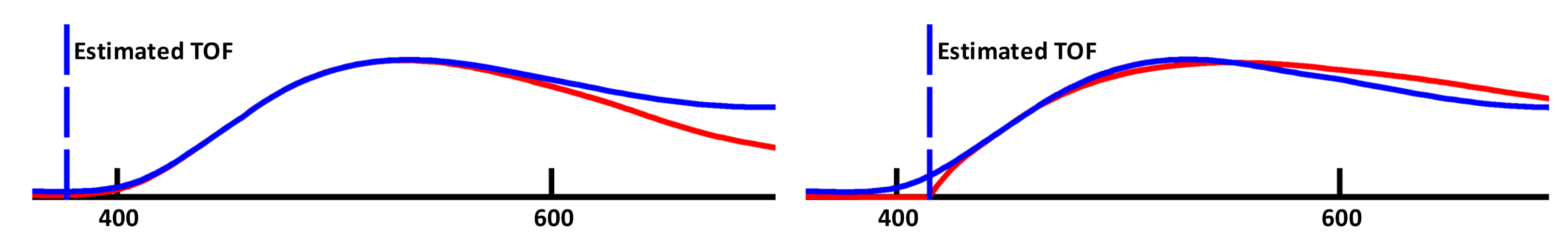
The existing TOF estimation methods are mostly aimed at stationary targets whose ultrasonic echo signals are complete and undistorted waveforms, as shown in Figure 1. However, in practical applications, it is often impossible for the target object to be completely stationary, and the target object is often a moving object. These conditions often lead to the distortion of the envelope waveform, resulting in inaccurate TOF estimation, as shown in Figure 2. Furthermore, inaccurate TOF estimation results often lead to inaccurate object localization or unstable object tracking. This paper analyzes the most distorted ultrasonic echo waveform, and the proposed system integrates various methods to handle TOF estimation in most distortion cases, as shown in Figure 2. Furthermore, the remaining distortion cases that lead to inaccurate TOF estimation are processed by the stage of object localization. The object localization stage integrates several methods to provide a more stable and smoother result for the localization and tracking of stationary and moving objects.
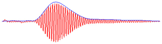
Figure 1.
Ideal shape of an ultrasonic waveform. (Blue line: echo envelope; red line: raw ultrasonic signal.)
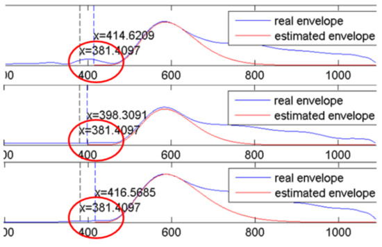
Figure 2.
Distorted shapes of envelope waveforms.
In this work, an ultrasonic array system consisting of one transmitter and five receivers for object localization and tracking is implemented. The transmitter transmits ultrasonic signals, and the five receivers receive the echo signals returned by the target. The localization system uses the proposed algorithm to analyze the raw data of the echo signal. First, the system detects whether there is an echo signal through a simple VAD algorithm and then starts to locate the target by the proposed algorithms. The demodulation algorithm with a low-pass filter is used to extract the envelope of the echo signal. In order to improve the accuracy and stability of TOF estimation, the GN model and the DE model are used to characterize the ultrasonic echo signal, and the NR algorithm is applied to fit the envelope curve to estimate the parameters of the models. Furthermore, the LM modification is applied to an NR algorithm to solve the ill-conditioned problem and improve the stability of the TOF estimation. Moreover, through the analysis of various distortion waveforms, a strategy is proposed to determine the optimal fitting area according to the ideal characteristics of the GN model and the DE model, which avoids the fitting of other distorted measurement data and reduces the deviation of TOF estimation. The next stage of the proposed system is to estimate the target position; thus a discrete EKF is designed to consider the interference of TOF estimation, which uses TOF to estimate the distance to locate the target position. Aiming at the problem of outliers in the measurement, the update process of EKF is improved, which effectively detects and eliminates outliers and improves the robustness of target tracking. In summary, the following algorithms are proposed in this study: one demodulation algorithm for envelope extraction, the NRLM with two models (GN and DE) for TOF estimation, and the EKF method with outlier rejection for object localization. These algorithms are used to build a system platform, and different algorithm combinations are realized in experiments to test the accuracy and stability of object localization and tracking. These methods are compared with each other to test which combination has the best performance. Experimental results show that the proposed ultrasonic range measurement method provides stable TOF estimation under the tolerable deviation and improves the performance of target localization and tracking in the application of human finger tracking.
The proposed system and algorithms can be applied to applications such as hand-writing systems on screens or smartphones and hand gesture recognition systems. One application for the proposed system is the large-scale non-touch screen. Especially in recent days, avoiding physical contact to prevent virus infection is an important issue. This system can be built in the business district for an interactive application with the people without physical contact. It is also a safe solution for healthcare professionals to perform contactless panel control in the operating room.
The rest of the paper is organized as follows. Section 2 gives the mathematical formulation of the proposed algorithms, including the VAD, demodulation for envelope extraction, the NRLM with the GN model and the DE model for TOF estimation, and the localization method of the EKF with outlier rejection. Section 3 presents the theoretical simulation for the performance comparison of the NRLM with the GN and DE models. The experimental description and result analysis of the system are described in Section 4. Finally, the conclusion is given in Section 5.
2. Mathematical Formulation of Object Localization and Tracking Algorithms
2.1. VAD Algorithm
The drive signal is a control signal from the outside of the system to the ultrasonic transmitter; thus its start time is known in one signal frame. Assuming that the surrounding environment to be detected is limited by the maximum distance, the maximum distance reached by the ultrasonic signal is a fixed value of . Assume that the ultrasonic speed is v and the sampling rate of the system is s. A signal frame f can be defined as the number of samples from the drive signal to the farthest target and back to the receiver, such that . Therefore, when the subsequent algorithm calculates a target position, it only needs to sample f after as a signal frame.
Because the beam shape of the ultrasonic sensor used in this system is a spherical waveform, the ultrasonic signal reflected by the test platform and the signal directly transmitted by the transmitter to the receiver will cause a blind area. The most important factors that determine the region of the blind area are the amplitude and the number of cycles of the trigger signal of the transmitter. As shown in Figure 3, signal 1 is the interference signal which results in the blind area, and signal 2 is the reflected signal of the detected object. When the amplitude and number of cycles of the trigger signal increase, the range of signal 1 and the region of the blind area increase. If the object is in the blind area, signal 2 is indistinguishable because it overlaps with signal 1 to form a single signal. If the object is not in the blind area, the waveform of the interference signal is fixed and stable in the same system. Only by avoiding this segment of the signal, the real available reflected signal of the object can be found.
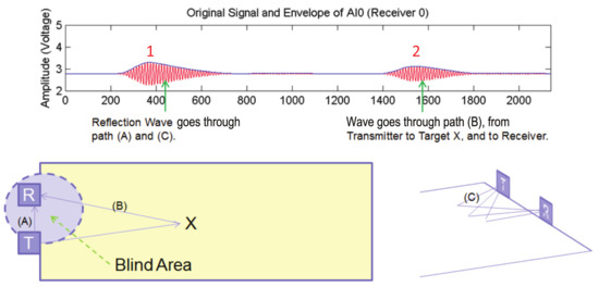
Figure 3.
Illustration of blind area. (Top): Interference signal 1 and reflected signal 2; (Bottom-left): Paths of interference signal (A) and reflected signal (B); (Bottom-right): Path of interference signal (C).
2.2. Envelope Extraction by Demodulation Algorithm
One critical point of the accuracy of the object localization is the precision of the start point time of the reflected ultrasonic signal, and the TOF can be calculated by the start point time. In general, the reflected ultrasonic signal is a set of 40 KHz signals, whose envelope must be captured first for the subsequent algorithm to calculate the start point time. To extract an envelope of the 40 KHz ultrasonic signal, the demodulation algorithm is proposed in this study. The concept of the demodulation algorithm is to extract the envelope signal by separating the high and low frequency of the original signal and retain the low-frequency part of the original signal through a low pass filter. The echo signal of the ultrasonic signal is modeled as:
where k is the time step, is the amplitude; that is, envelope, is the center frequency of ultrasonic, and is the phase shift.
Let (1) be multiplied by a sinusoidal signal and a cosine signal whose frequency is the same as that of the ultrasonic signal to generate and , the results can be obtained as follows:
In (2) and (3), the original signal is divided into two parts, the low-frequency part with , and the high-frequency part with . Therefore, a low-pass filter with a cut-off frequency around can be designed to filter out the high-frequency part, and the following results can be obtained:
where and are the sample signals after passing through a low pass filter. As a consequence, the envelope can be obtained as follows:
2.3. TOF Estimation
The algorithm of the whole system focuses on finding the start point of the reflected ultrasound signal, namely TOF estimation. In this section, the NRLM algorithm based on the GN model and the DE model is proposed and applied in the system.
2.3.1. The Envelope Model of Ultrasonic Echo Signal
In general, the GN form of the ultrasonic envelope can be modeled as an analytical expression [32], such that:
where , is the TOF, accounts for the amplitude of the ultrasonic echo signal, and p are shape parameters of the specific ultrasonic transducer, and t is time. The model uses the parabolic term and the exponential decay term to characterize the envelope waveform.
The other model used in this study is the DE model [33] such that:
where , is the TOF, accounts for the amplitude of the ultrasonic echo signal, and are the decay factors (it is noted that must be larger than ), and t is time. The DE model characterizes the envelope by two exponential terms.
It is noted that the main difference between the GN model and the DE model is that they characterize the rising edge (the reign from TOF to peak) of the echo in different methods. The GN model characterizes the rising edge as a parabolic term, while the DE model characterizes the rising edge as a concave downward curve term. These two different models are applied in the proposed system to test which one is more suitable to cooperate with other algorithms in this study, and the comparison results are shown in Section 3 and Section 4.
2.3.2. NRLM Algorithm for TOF Estimation
To estimate the unknown parameters in (7) and in (8), the nonlinear curve-fitting algorithm using NRLM is applied on the GN model and the DE model in this study.
First, the algorithm to estimate in the GN model is developed. Suppose , is the measurement value of the envelope data in each frame. To formulate the curve-fitting problem with the GN model (7), the object function can be constructed as follows:
Furthermore, the nonlinear LS problem can be obtained such that:
which represents the minimum summation of the squared errors between measurement values and model values at the corresponding points in time. An argument vector can be constructed as: where , and the object function (9) can be rewritten as follows:
To apply the NR algorithm for a nonlinear LS problem, the Jacobian matrix of , the gradient , and Hessian matrix of are needed to be calculated first. The Jacobian matrix is as follows:
where in this study, and , , , and , respectively. Therefore, the Jacobian matrix of this problem is a matrix with elements as follows:
where is the th element of the Jacobian matrix , and . The next step is to calculate the gradient as follows:
Furthermore, the Hessian matrix is defined as:
and the th element of the Hessian matrix can be expressed by using indices k and j such that:
where is defined as the th element of matrix . Therefore, the Hessian matrix can be obtained as the following form:
As a consequence, the recursive formula for the NR algorithm applied to the nonlinear LS problem is as follows:
where the notation and denote the kth and th time steps. In general, the term in (21) is significantly small because it contains the second derivative terms and can be ignored in practical applications. However, ignoring the term in (21) may cause to become a singular matrix and make the system crash. This problem can be solved by using the LM modification, which adds a sufficiently large number into the diagonal of such that:
This term can make sure that the search always points to the descent direction, and it can be viewed as an approximation to in (22). Therefore, (23) is the ongoing, recursive formula for the TOF estimation .
The above procedure also can be applied on the DE model, and (23) is modified as:
where
to estimate the TOF . (23) and (24) are tested with the aforementioned algorithms in this study, and the performances of the simulation and experimental results are compared in Section 3 and Section 4, respectively.
2.3.3. Determination of Suitable Fitting Window
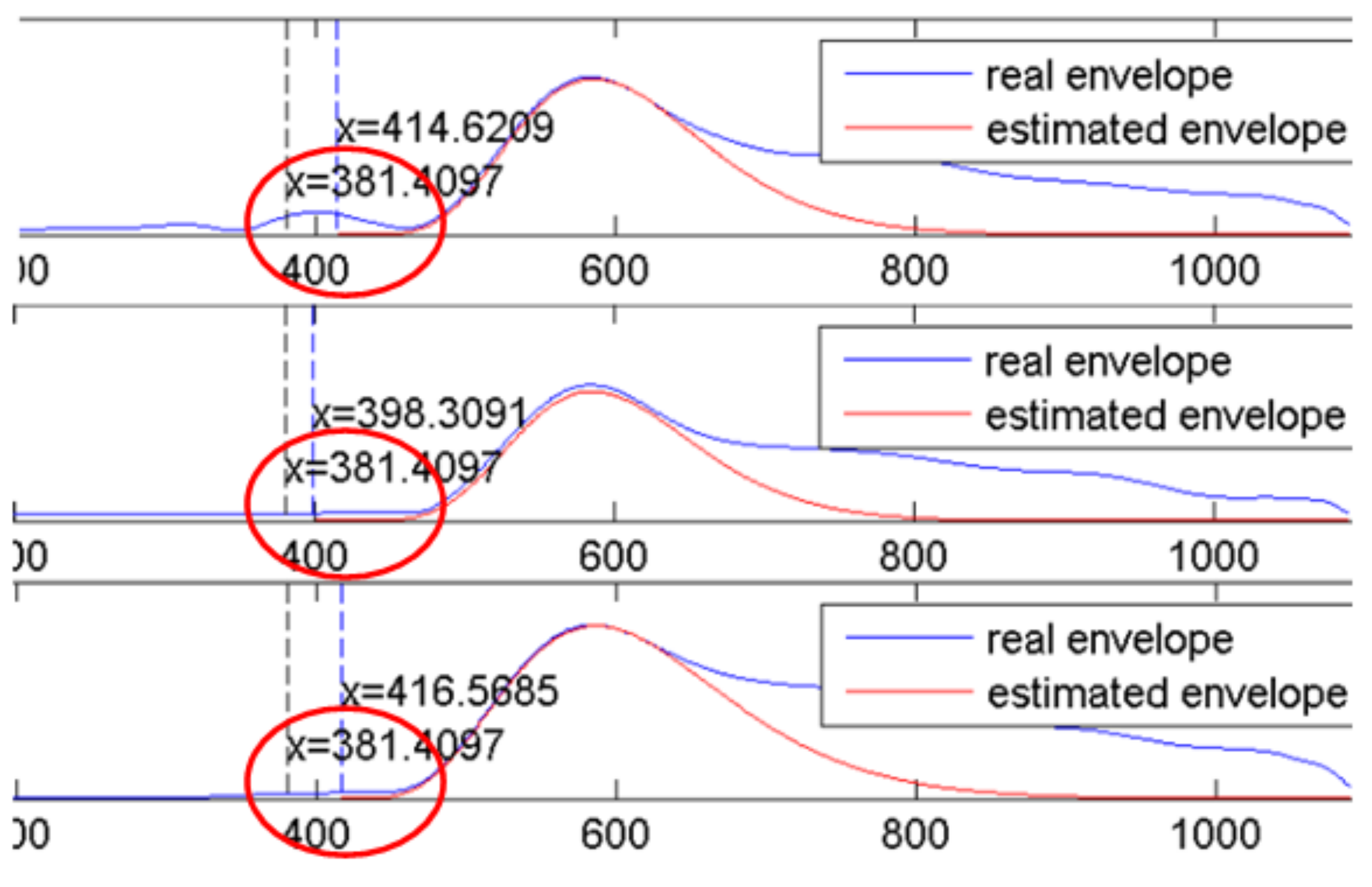
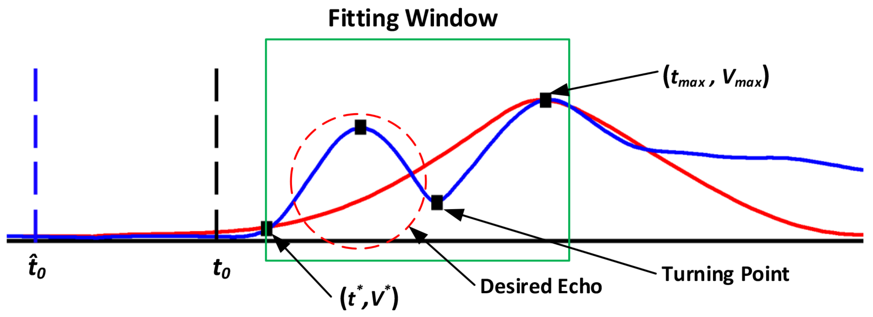
In the proposed system, when the amplitude of the ultrasonic echo signal is sufficiently large to be detected, the target is judged to exist by the system, and the TOF is estimated by the proposed algorithm. However, the waveform of the ultrasonic echo signal is always distorted because of different reflective surfaces, which results in the multiple-peaks phenomenon and interference results of TOF estimation. Therefore, instead of fitting the entire envelope data, a suitable fitting window located on the expected peak according to the mathematical properties of the envelope model is better. For example, reconsidering the GN model (7), which has only one peak value, the curve from the peak to the beginning is monotonically decreasing; that is, there is no turning point. Therefore, as shown in Figure 4, the ideal shape of the waveform in the fitting window should be a single peak and monotonically decrease from the peak; otherwise, a large fitting error will be caused, and the accuracy of TOF estimation will be affected, as shown in Figure 5.
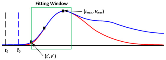
Figure 4.
Ideal shape of envelope waveform. (Blue line: echo envelope; red line: curve-fitting result.)

Figure 5.
Double peaks phenomenon of envelope waveform. (Blue line: echo envelope; red line: curve-fitting result.)
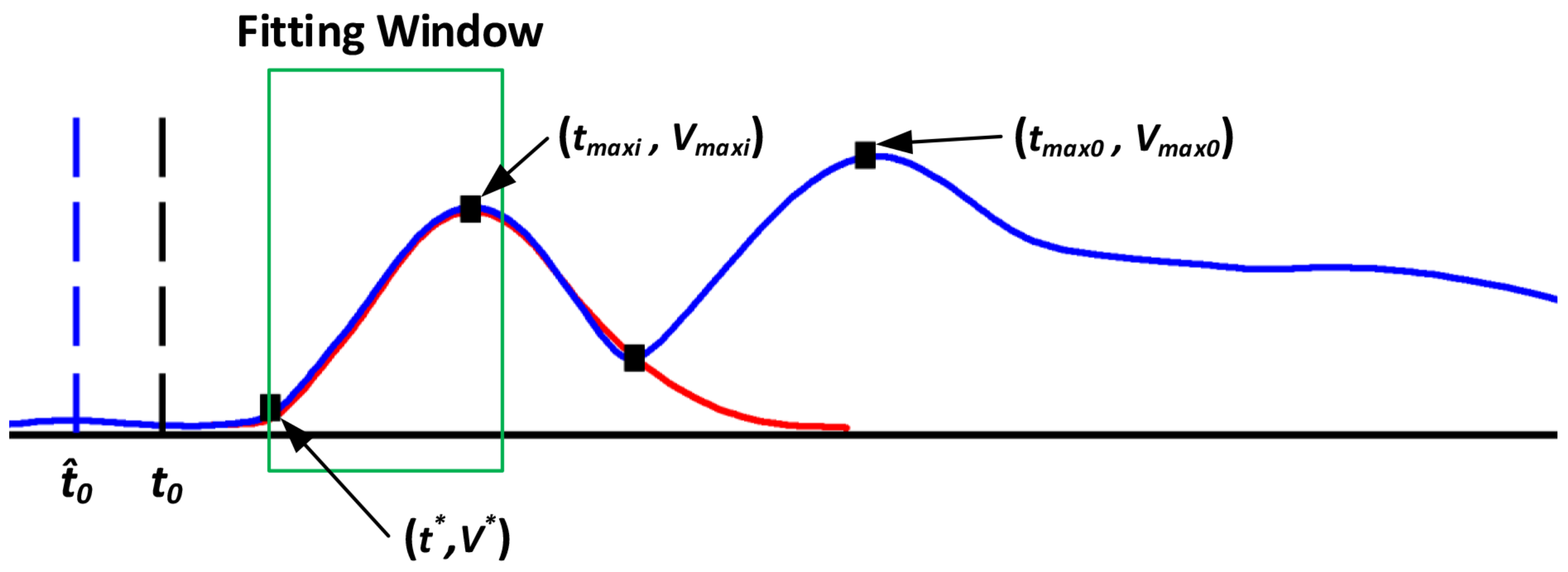
To solve the problem of an incorrect fitting window with multi-peaks, a three-step procedure is proposed in this study. In Figure 4, Figure 5 and Figure 6, the blue line is the echo envelope, the red line is the result of curve-fitting, is the estimated TOF by (23) or (24), is the ground truth of TOF, which is calculated from target coordinate measured manually, is the peak value of echo envelope, and is the instant that characterizes the onset of echo envelope, which is calculated by the two-maximums algorithm [15]. The size of the fitting window is defined from to , where n is a suitable number. The three-step procedure is presented as follows:
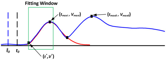
Figure 6.
Curve-fitting result of envelope waveform in the desired region. (Blue line: echo envelope; red line: curve-fitting result).
- (1)
- Set the maximum amplitude detected for the first time as the initial value , and find the corresponding by the two-maximums algorithm.
- (2)
- In the ith iteration, check if the waveform from to is a monotonic decrease. If it is a monotonic decrease, then go to step 3.
- (3)
Through the above three-step process, the suitable fitting window can be found, and the best fitting result can be obtained, as shown in Figure 6.
2.4. Object Localization and Tracking Algorithm
When the TOFs of all sensor channels are estimated by the NRLM methods with the GN model or the DE model, the position of the target can be estimated by these TOFs. In this section, the NRLM algorithm can also be used in target position estimation. In addition, the EKF algorithm is also proposed for object localization and tracking. The performance of these two proposed methods is compared with the other methods in Section 4.
2.4.1. NRLM Algorithm for Object Localization
Suppose v is the wave propagation speed of ultrasonic, is the target object position, which is unknown, is the position of the ultrasonic transmitter, is the position of the ultrasonic receiver where , and m is the number of receivers, and , and (in general applications, or 3), and is the traveling time, which can be measured from the transmitter to the object and back to the receiver i. The round trip equation can be formulated as follows:
which presents the traveling time from the transmitter to the object and back to the receiver i. Therefore, the problem can be constructed as the minimum summation of the squared errors between measured traveling times with the corresponding receivers such that:
From Section 2.3.2, a similar procedure can be applied to solve this problem by a recursive formula to estimate the object position .
2.4.2. EKF Algorithm for Object Localization and Tracking
In this section, the EKF algorithm is used to estimate the position and velocity of the target. Suppose the state where is the position coordinate and is the velocity of target. The state transition equation can be written as follows:
where
where t is the transition time, the notations and denote the kth and th time steps, and is the state noise, which is Gaussian distribution with zero mean and diagonal covariance matrix . The measurement equation is:
where , and is the observation noise, which is Gaussian distribution with zero mean and diagonal covariance matrix .
When the TOFs are obtained from each channel, outliers may occur when the echo distortion is under serious conditions, such as complex shaped targets or target movement, affecting the performance of the EKF. A reliable and efficient method is provided in [34] for outlier detection. The prediction step (31) and (33) in the proposed EKF are modified as follows:
where , , , and is the noise variance of . The Kalman update process is as follows:
where
and is the ith element of , is the ith element of , and is a weighting such that:
and the mth element of diagonal of is such that:
where is the mth row of the matrix . Here, is the Kalman gain, is the posterior covariance of the residual prediction error, and is suggested in [34].
In the Kalman update process, (42) presents that if the prediction error in increases, the weighting of that data sample will decrease. If the prediction error is too large and dominates the denominator, the weighting will become very small. Furthermore, the posterior covariance of the residual prediction error will become very small to result in a very small Kalman gain and decrease the influence of the data sample when predicting .
3. Theoretical Comparison of TOF Estimation with Simulation
To compare the performances of TOF estimation by the proposed NRLM algorithm with the GN model and the DE model, the envelope data extracted from a complete and undistorted echo signal of ultrasonic, such as Figure 1, is used to test the simulation with different signal-to-noise-ratios (SNR). In the simulation, the performances are tested with the root mean square error (RMSE) between the estimated TOF and the real TOF. The RMSE is defined as follows:
where is the estimated TOF, t is the real TOF, and is the number of simulation runs at the specified noise level. In the simulation, the noises are added to the envelope signal with different SNRs, which are defined as follows:
where is the maximum amplitude of the envelope and is the standard deviation of the noise. The simulation results are presented in Figure 7. It is observed that the proposed NRLM algorithm with the DE model has better performance than that with the GN model when SNR is low, and they have similar performances when SNR is high. Therefore, it can be concluded that the proposed NRLM algorithm with the DE model has superior flexibility than that with the GN model.
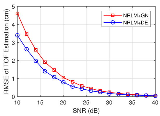
Figure 7.
Simulation results of the TOF estimation with different SNRs.
4. Experiment Results
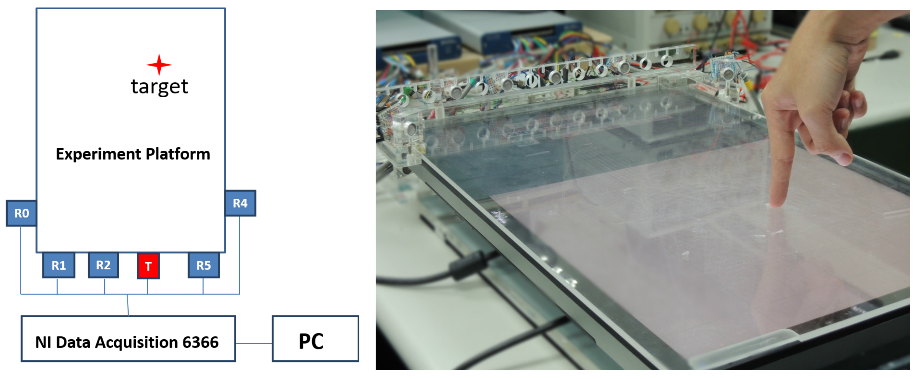
The architecture of the experiment system using ultrasonic sensors and the real experiment platform are shown in Figure 8. As shown in the left figure of Figure 8, there are one transmitter (red) and five receivers (blue) mounted on the edge of a 60 × 38 platform with a U-shaped sensor rack. The ultrasonic sensors used in this system are Pro-wave 400PT160, which is a transceiver with a center frequency of 40 KHz such that they can operate as the transmitter or the receiver [35]. The NI data acquisition (DAQ USB-6366) is connected between the computer and all sensors. The DAQ is used to drive the transmitter by a computer with a rectangular burst consisting of eight cycles, acquire the raw data of analog echo signal from sensors, and convert these analog data into digital data and send them to the computer. In the following subsections, there are three cases to be tested such that:

Figure 8.
(Left): The architecture of the experimental system; (Right): The photo of the real experiment environment of the ultrasonic platform with the target as a human finger.
- Case 1:
- The localization target is a stationary marker pen that stands vertically on the platform at measured coordinates. This testing object is stationary and has a smooth surface.
- Case 2:
- The localization target is one human index finger stationary pointing vertically to the platform at measured coordinates. This testing object is stationary and has an uneven surface.
- Case 3:
- The system will track one moving human finger with different trajectories, and the index finger is pointing vertically to the platform. This testing object is moving and has an uneven surface.
There are 700 testing frames in Case 1 and Case 2 and 300 testing frames in Case 3.
4.1. The Performance of TOF Estimation
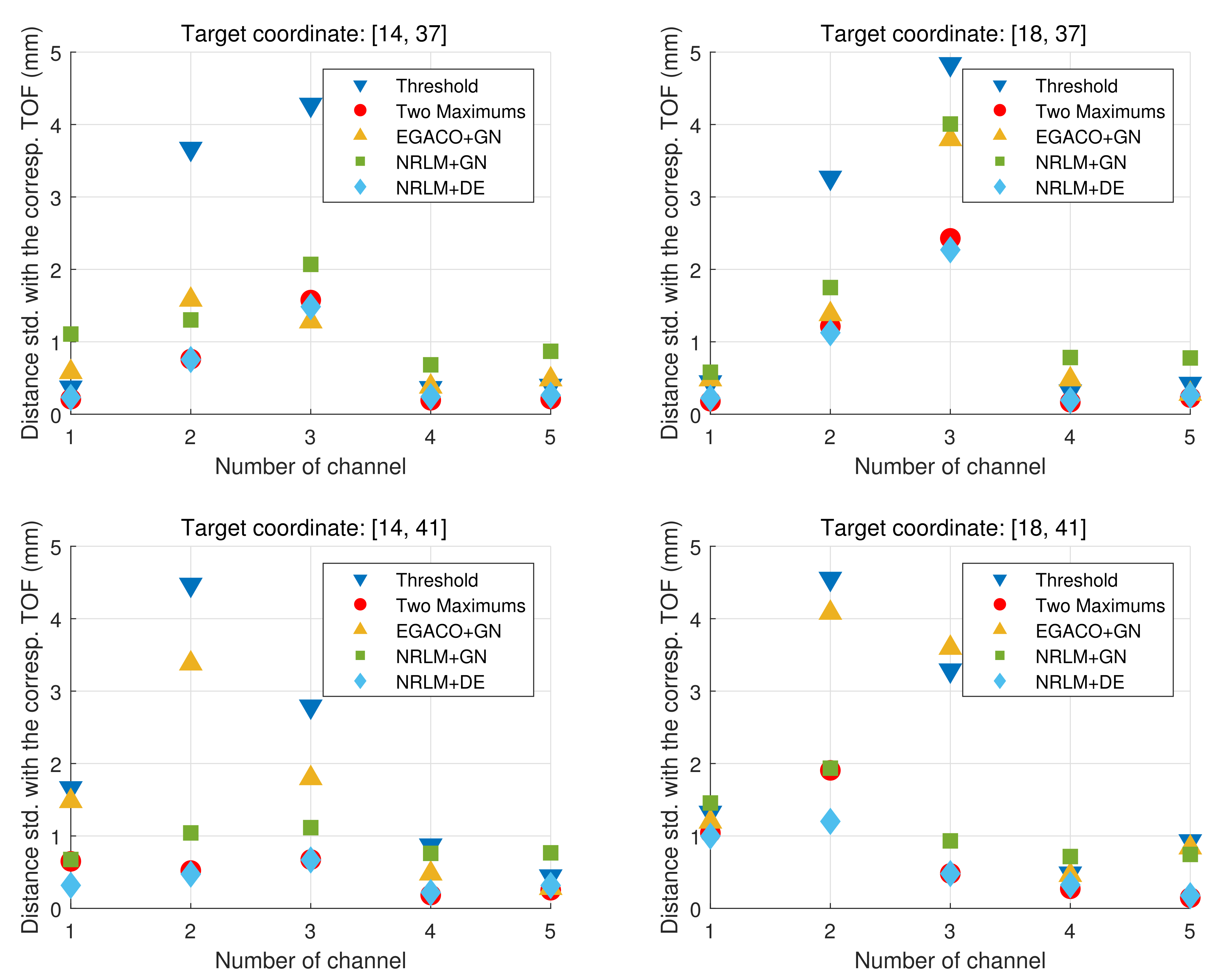
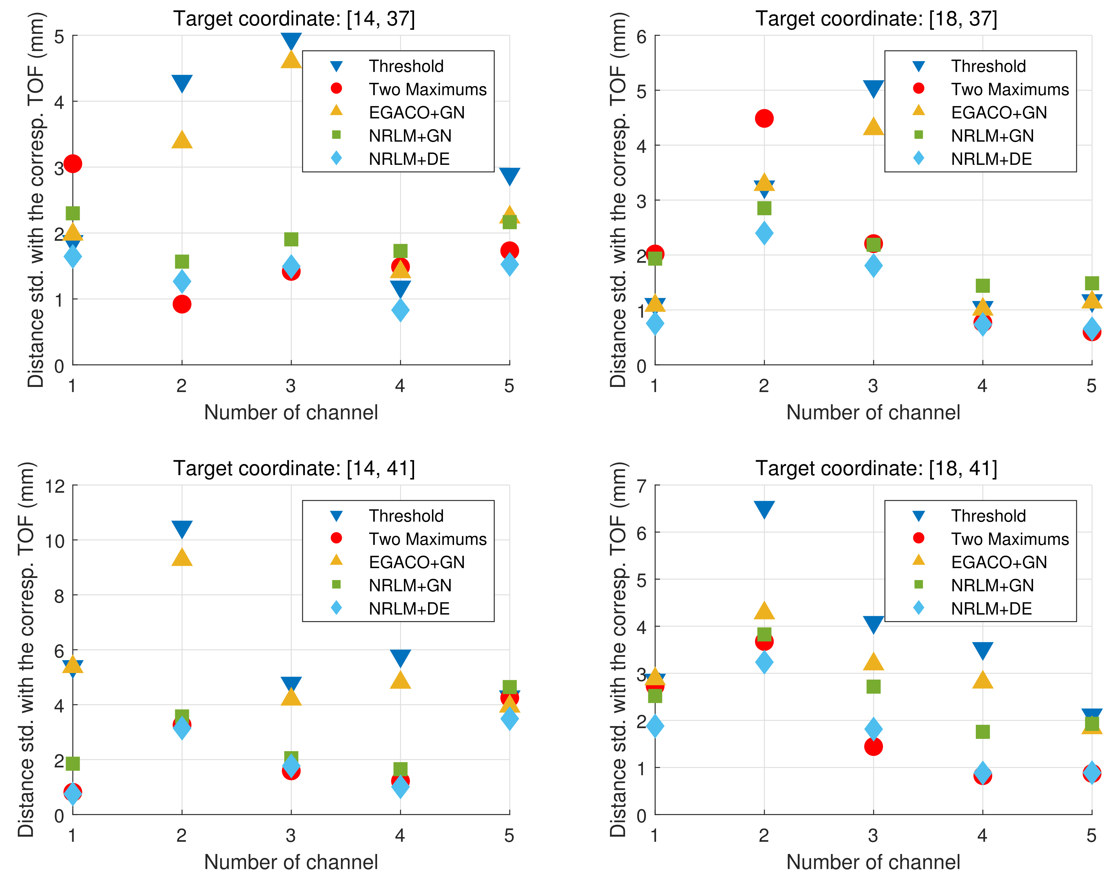
In this section, the fixed threshold method [12,13], the two-maximums algorithm [15], the energy genetic-ant colony optimization-three-cycle (EGACO) algorithm with the GN model [21], the proposed NRLM algorithm with the GN model (23), and the proposed NRLM algorithm with the DE model (24) are tested to compare the standard deviations of the TOF estimation in Case 1 and Case 2, where the targets are all stationary. All approaches tested here are applied to the same fitting window. The standard deviations of the testing results of five receiver channels are shown in Figure 9 and Figure 10. It is noted that the vertical axis presents the standard deviations of distances with the corresponding TOFs in Figure 9 and Figure 10 for intuitive observation.
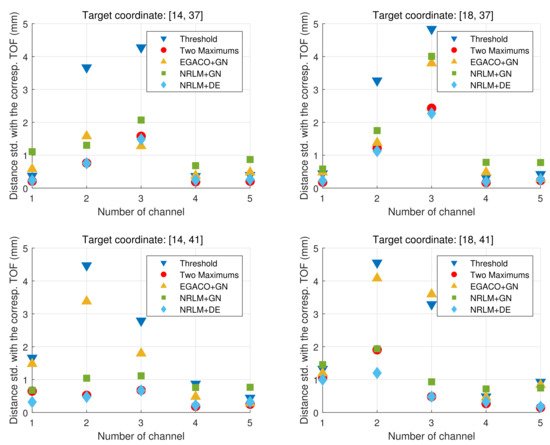
Figure 9.
Case 1 (marker pen): Standard deviations of distances with the corresponding TOFs of different methods among five receiver channels. (▾): threshold method; (•): two-maximums algorithm; (▴): EGACO algorithm with GN model; (■): NRLM algorithm with GN model; (⧫): NRLM algorithm with DE model. (Vertical coordinate unit: mm).
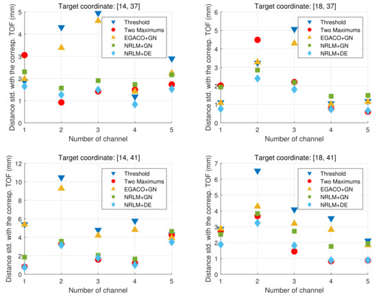
Figure 10.
Case 2 (human index finger): Standard deviations of distances with the corresponding TOFs of different methods among five receiver channels. (▾): threshold method; (•): two-maximums algorithm; (▴): EGACO algorithm with GN model; (■): NRLM algorithm with GN model; (⧫): NRLM algorithm with DE model. (Vertical coordinate unit: mm).
It is observed that the threshold method has a larger variation in TOF estimation when it is the target in both cases. Since the threshold method uses a fixed threshold value to detect TOF, it can not handle most situations. Regardless of whether the target is a pen or a human finger, the amplitude of the interference wave, which is greater than the threshold value, seriously affects the estimation results and produces some outliers. The results of TOF estimation of the two-maximums algorithm are relatively stable and more accurate than those of the threshold method because it applies linear interpolation based on the envelope model on the rising edge to estimate the TOF, and the rising edge is also located in the ideal echo region from the method in Section 2.3.3. However, the linear interpolation used in the two-maximums algorithm is very sensitive to changes in the slope of the rising edge, resulting in corresponding interference to TOF estimation.
In Figure 9 and Figure 10, it is observed that the proposed NRLM algorithm with the DE model has better performance than the other methods in most cases, including the EGACO algorithm with the GN model and the proposed NRLM algorithm with the GN model. The EGACO uses the GN model and estimates the TOF by judging the maximum energy position of the signal. The result of EGACO is similar to that of the threshold method in many cases because it estimates the TOF by signal energy, which is easily affected by the shape of the signal, especially when the object is in the non-stationary state. The curve-fitting results of the NRLM algorithm with the GN model and the DE model are shown in Figure 11. The GN model characterizes the actual envelope better than the DE model, such that the residual error of curve-fitting using (7) is smaller than that of (8). However, the GN model is more sensitive to the variation of the measured echo signal because it fits the onset of the echo well and interferes with the TOF. On the other hand, although the TOF estimation of the DE model has a certain deviation, the rising edge of the model is less sensitive to the variation of the echo, which is consistent with the simulation result in Section 3. Therefore, it can be concluded that the NRLM algorithm with the DE model provides a more stable TOF estimation than other methods, and the TOF data estimated by the NRLM algorithm with the DE model is used in all cases in the object localization and tracking in Section 4.2.

Figure 11.
Curve-fitting results of the GN model and the DE model. (Left): NRLM algorithm with the GN model; (Right): NRLM algorithm with the DE model. (Blue line: original echo signal; red line: envelope model by the proposed methods.)
4.2. The Performance of Object Localization and Tracking
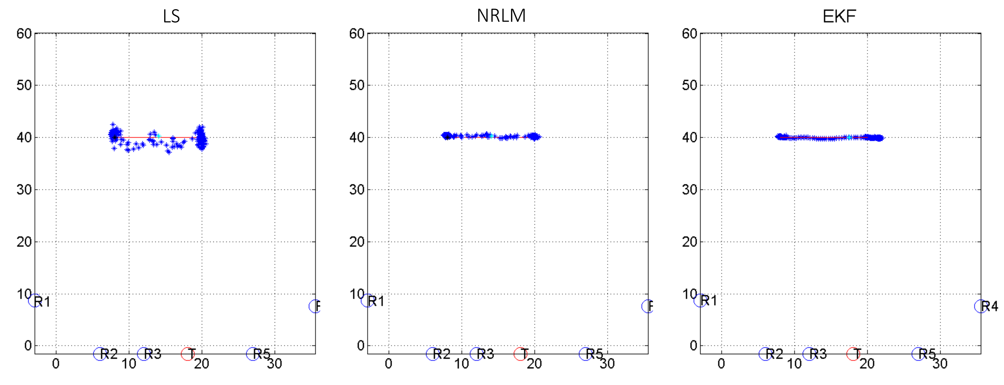
In this section, the concept of the LS method [27], the proposed NRLM method, and the proposed EKF method are used to estimate the target position. The TOF results of all the five receiver channels are used among the three methods, and the issue of outlier rejection is then discussed.
Table 1 and Table 2 present the RMSE of the target position with three methods in Cases 1 and 2 to show the accuracy of the object localization methods. Table 3 and Table 4 present the standard deviations of the target position with the three methods in Cases 1 and 2 to show the stability of the object localization methods. It is observed that most RMSEs and all standard deviations of the EKF method are much smaller than those of the other methods in both cases. Therefore, the proposed EKF method has better performance in both accuracy and stability than the other methods for object localization.

Table 1.
Case 1—RMSE of target coordinates (X, Y) for the marker pen (unit: cm).
Table 2.
Case 2—RMSE of target coordinates (X, Y) for human index finger (unit: cm).
Table 3.
Case 1—Standard deviations of target coordinates (X, Y) for the marker pen (unit: cm).
Table 4.
Case 2—Standard deviations of target coordinates (X, Y) for human index finger (unit: cm).
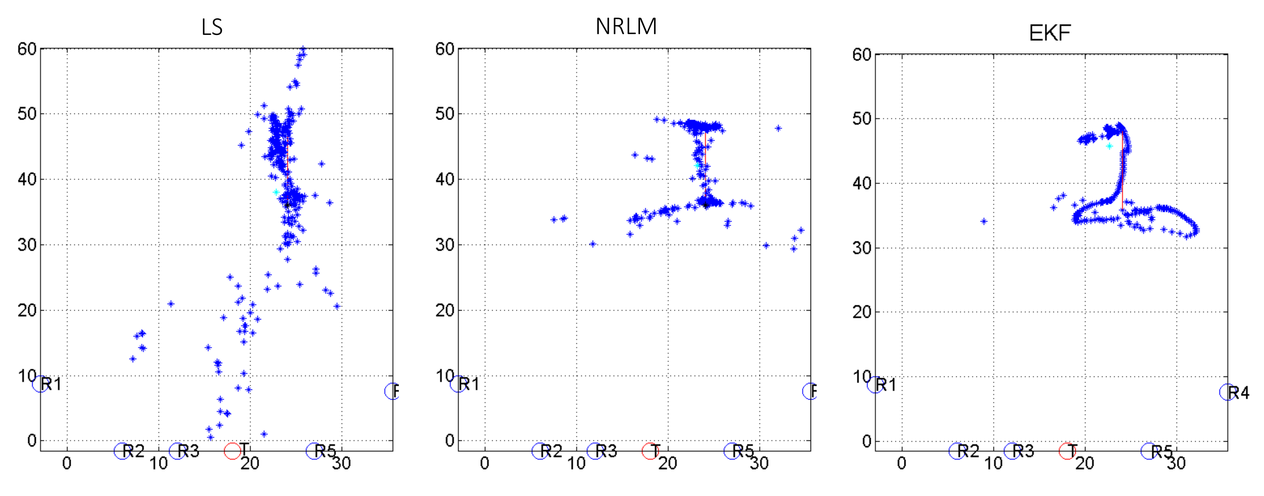
Figure 12, Figure 13 and Figure 14 present the results of target tracking with different moving directions for Case 3, which are denoted as Case 3-1, Case 3-2, and Case 3-3. It should be noted that in all test trajectories of Case 3, the finger stops for a period of time at the start and end points before and after the movement. In the LS method, there is a system matrix containing distance estimation, which increases the uncertainty of the estimation and easily causes ill-conditioned problems. Because the round-trip model does not include any distance estimation, the NRLM method is superior to the LS method. However, the NRLM method only estimates coordinates based on the current TOF data, and the estimation results are directly affected by the measurement noise. Although the performance of the NRLM method and the EKF method in the stationary state of the target is similar, the EKF estimates the position of the target based on the previous state of the target, and inherently considers the interference of the measurement, which can provide more stable and smoother localization and tracking of the moving target. It is noticed that in Figure 14, the tracking in the x-direction is delayed more than the tracking in the y-direction. This is because the geometry of the ultrasound platform structure makes the variance in the x-direction larger than that in the y-direction [36], which can also be observed in Table 2 and Table 4.
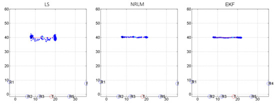
Figure 12.
Case 3-1: Target moves from (8, 40) to (20, 40), the velocity in the x-direction is about 1 cm/s. (Blue dots: the estimated coordinates of moving target; red line: the reference target trajectory.)
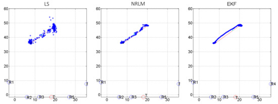
Figure 13.
Case 3-2: Target moves from (8, 36) to (20, 48), the velocity of the target is about cm/s. (Blue dots: the estimated coordinates of moving target; red line: the reference target trajectory.)
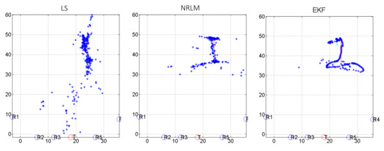
Figure 14.
Case 3-3: Target moves from (20, 36) to (20, 48), the velocity in the y-direction is about 1 cm/s. (Blue dots: the estimated coordinates of moving target; red line: the reference target trajectory.)
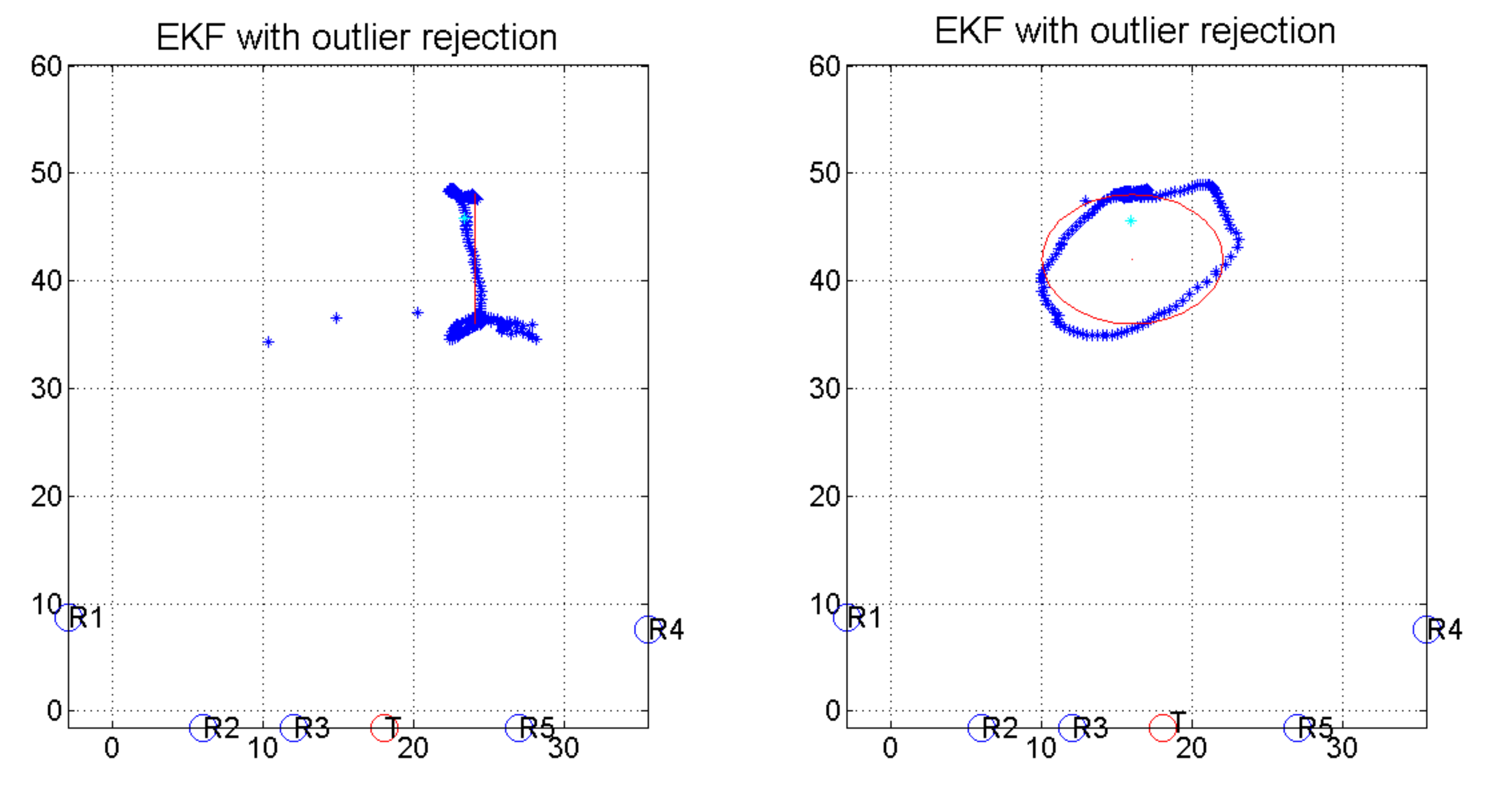
Here, the outlier issue is reconsidered in Case 3-3. When the target moves from (20, 36) to (20, 48), it is observed that sometimes the echo signal is severely distorted and results in generating several outliers in the measurement data. The outliers have a great influence on the tracking performance of the EKF method. In Figure 15, the outlier rejection method proposed in Section 2.4.2 is used to improve the tracking performance of the target. As shown in the left figure of Figure 15, it can be observed that when the outliers are detected and eliminated, the variance of the x-coordinate is relatively small, and the estimated target trajectory can follow the desired path more smoothly and more consistently than that in the right figure of Figure 14. It is noted that since there are no obvious outliers in the measurement by the EKF method in Case 3-1 and Case 3-2, the results of the tracking will be similar before and after outlier rejection.
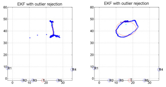
Figure 15.
(Left): The target moves from (20, 36) to (20, 48), the velocity in the y-direction is about 1 cm/s; (Right): The target moves in a circle with center at (16, 42), both the start point and the end point are at (16, 48). (Blue dots: the estimated coordinates of moving target; red line: the reference target trajectory.)
Another test trajectory is shown in the right figure of Figure 15. The estimated target coordinates are around the reference trajectory. However, there is a delay in the x-direction near the end point. This is caused by the constant occurrence of outliers as the target moves. Because the Kalman gain is smaller in the presence of outliers, the estimated coordinates are closer to the predicted trajectory.
In Figure 15, it can be observed that there are differences between the real trajectories and the estimated trajectories, but the estimated tracking trajectories are quite stable, which means that the proposed algorithm can be fairly stable to localize the detected object. In this work, the key issue for object localization is not only to directly estimate the accurate position but also to estimate the stable position. In reality, position estimation is prone to deviation due to the influences of various factors, such as the size of the sensors and the geometry of sensor positions. It is not practical to consider these factors because it makes the system complicated and not easy to solve. However, in a fixed system, these influences are also fixed and always result in a fixed offset in position estimation with a fixed position. Thus, even if there is an error between the position estimation and the real position, the error can be directly compensated by an offset calibration to achieve the correct object localization and tracking. In Figure 15 and Table 3 and Table 4, it can be observed that the standard deviations of the EKF method are very small. The smaller the standard deviation, the better the stability of the position estimation. Therefore, although there is a difference between the real trajectories and the estimated trajectories, the difference can be easily compensated by offset calibration because of the good stability of position estimation.
5. Conclusions
An ultrasonic array system consisting of one transmitter and five receivers for object localization and tracking is proposed in this paper. The system uses the VAD algorithm to detect the target’s echo signal and locate the target. The envelope is then extracted by the demodulation algorithm, and the TOF estimation is performed by the NRLM algorithm with the GN model or the DE model. Furthermore, the detected object can be located by the NRLM algorithm or the EKF algorithm with outlier rejection. In this study, these proposed methods are compared and experimentally evaluated in different scenarios for TOF estimation and tracking on target position. The NRLM algorithm that uses nonlinear curve-fitting provides a more reasonable TOF than other methods that use linear interpolation. Although the GN model is more suitable for the rising edge than the DE model, the TOF estimation of the GN model is more sensitive to the variation of the rising edge. The EKF method uses previous states to decrease the influence of the current interference of measurement. Moreover, outlier rejection provides a more stable and smoother result for the localization and tracking of moving targets. Therefore, the experiment results verify that the NRLM algorithm with the DE model has the best performance for TOF estimation, and the EKF algorithm outperforms the other methods in object localization.
Author Contributions
Conceptualization, C.-W.J. and J.-S.H.; methodology, C.-W.J. and J.-S.H.; software, C.-W.J.; validation, C.-W.J.; formal analysis, C.-W.J. and J.-S.H.; investigation, C.-W.J. and J.-S.H.; resources, C.-W.J. and J.-S.H.; data curation, C.-W.J.; writing—original draft preparation, C.-W.J.; writing—review and editing, C.-W.J.; visualization, C.-W.J.; supervision, C.-W.J. and J.-S.H.; project administration, C.-W.J. and J.-S.H.; funding acquisition, C.-W.J. and J.-S.H. All authors have read and agreed to the published version of the manuscript.
Funding
This research was funded by the Ministry of Science and Technology, Taiwan (Grant Number: MOST 108-2221-E-009-122-MY2).
Institutional Review Board Statement
Not applicable.
Informed Consent Statement
Not applicable.
Data Availability Statement
The data presented in this study are included within the article.
Conflicts of Interest
The authors declare no conflict of interest.
References
- Yu, L.; Wang, X.; Hou, Z.; Du, Z.; Zeng, Y.; Mu, Z. Path Planning Optimization for Driverless Vehicle in Parallel Parking Integrating Radial Basis Function Neural Network. Appl. Sci. 2021, 11, 8178. [Google Scholar] [CrossRef]
- Ji, H.; Cui, X.; Gao, Y.; Ge, X. 3-D Ultrasonic Localization of Transformer Patrol Robot Based on EMD and PHAT-β1 Algorithms. IEEE Trans. Instrum. Meas. 2021, 70, 1–10. [Google Scholar]
- Zeng, Q.; Kuang, Z.; Wu, S.; Yang, J. A Method of Ultrasonic Finger Gesture Recognition Based on the Micro-Doppler Effect. Appl. Sci. 2019, 9, 2314. [Google Scholar] [CrossRef] [Green Version]
- Mozumi, M.; Hasegawa, H. Adaptive Beamformer Combined with Phase Coherence Weighting Applied to Ultrafast Ultrasound. Appl. Sci. 2018, 8, 204. [Google Scholar] [CrossRef] [Green Version]
- Kaltsoukalas, K.; Makris, S.; Chryssolouris, G. On generating the motion of industrial robot manipulators. Robot.-Comput.-Integr. Manuf. 2015, 32, 65–71. [Google Scholar] [CrossRef]
- Choi, H.; Seong, W.; Yang, H. Source Type Classification and Localization of Inter-Floor Noise with a Single Sensor and Knowledge Transfer between Reinforced Concrete Buildings. Appl. Sci. 2021, 11, 5399. [Google Scholar] [CrossRef]
- Zhuo, D.-B.; Cao, H. Fast Sound Source Localization Based on SRP-PHAT Using Density Peaks Clustering. Appl. Sci. 2021, 11, 445. [Google Scholar] [CrossRef]
- Chen, H.; Ballal, T.; Muqaibel, A.H.; Zhang, X.; Al-Naffouri, T.Y. Air Writing via Receiver Array-Based Ultrasonic Source Localization. IEEE Trans. Instrum. Meas. 2020, 69, 8088–8101. [Google Scholar] [CrossRef]
- Kim, K.; Wang, S.; Ryu, H.; Lee, S.Q. Acoustic-Based Position Estimation of an Object and a Person Using Active Localization and Sound Field Analysis. Appl. Sci. 2020, 10, 9090. [Google Scholar] [CrossRef]
- Kishimoto, T.; Woo, H.; Komatsu, R.; Tamura, Y.; Tomita, H.; Shimazoe, K.; Yamashita, A.; Asama, H. Path Planning for Localization of Radiation Sources Based on Principal Component Analysis. Appl. Sci. 2021, 11, 4707. [Google Scholar] [CrossRef]
- Sabatini, A.M. A digital-signal-processing technique for ultrasonic signal modeling and classification. IEEE Trans. Instrum. Meas. 2001, 50, 15–21. [Google Scholar] [CrossRef]
- Vemuri, A.T. Using a fixed threshold in ultrasonic distance-ranging automotive applications. Analog. Appl. J. 2012, 3Q, 19–23. [Google Scholar]
- Yi, D.; Jin, H.; Kim, M.C.; Kim, S.C. An Ultrasonic Object Detection Applying the ID Based on Spread Spectrum Technique for a Vehicle. Sensors 2020, 20, 414. [Google Scholar] [CrossRef] [PubMed] [Green Version]
- Hammad, A.; Hafez, A.; Elewa, M.T. A LabVIEW Based Experimental Platform for Ultrasonic Range Measurements. DSP J. 2007, 6, 1–8. [Google Scholar]
- Raya, R.; Frizera, A.; Ceres, R.; Calderón, L.; Rocon, E. Design and evaluation of a fast model-based algorithm for ultrasonic range measurements. Sens. Actuators Phys. 2008, 148, 335–341. [Google Scholar] [CrossRef]
- Weenk, D.; van Beijnum, B.J.F.; Droog, A.; Hermens, H.J.; Veltink, P.H. Ultrasonic range measurements on the human body. In Proceedings of the 2013 Seventh International Conference on Sensing Technology, Wellington, New Zealand, 3–5 December 2013. [Google Scholar]
- Barshan, B. Fast processing techniques for accurate ultrasonic range measurements. Meas. Sci. Technol. 2000, 11, 45–50. [Google Scholar] [CrossRef]
- Parrilla, M.; Anaya, J.; Fritsch, C. Digital signal processing techniques for high accuracy ultrasonic range measurements. IEEE Trans. Instrum. Meas. 1991, 40, 759–763. [Google Scholar] [CrossRef]
- Marioli, D.; Narduzzi, C.; Offelli, C.; Petri, D.; Sardini, E.; Taroni, A. Digital time-of-flight measurement for ultrasonic sensors. IEEE Trans. Instrum. Meas. 1992, 41, 9–97. [Google Scholar] [CrossRef]
- Queirós, R.; Alegria, F.C.; Girão, P.S.; Serra, A.C. Cross-correlation and sine-fitting techniques for high resolution ultrasonic ranging. IEEE Trans. Instrum. Meas. 2010, 59, 3227–3236. [Google Scholar] [CrossRef]
- Zheng, D.; Hou, H.; Zhang, T. Research and realization of ultrasonic gas flow rate measurement based on ultrasonic exponential model. Ultrasonics 2016, 67, 112–119. [Google Scholar] [CrossRef] [PubMed]
- Paul, A.; Sato, T. Localization in Wireless Sensor Networks: A Survey on Algorithms, Measurement Techniques, Applications and Challenges. J. Sens. Actuator Netw. 2017, 6, 24. [Google Scholar] [CrossRef] [Green Version]
- Wu, S.; Zhang, S.; Huang, D. A TOA-Based Localization Algorithm With Simultaneous NLOS Mitigation and Synchronization Error Elimination. IEEE Sens. Lett. 2019, 3, 1–4. [Google Scholar] [CrossRef]
- Azmi, N.A.; Samsul, S.; Yamada, Y.; Yakub, M.F.M.; Ismail, M.I.M.; Dziyauddin, R.A. A Survey of Localization using RSSI and TDoA Techniques in Wireless Sensor Network: System Architecture. In Proceedings of the 2018 2nd International Conference on Telematics and Future Generation Networks (TAFGEN), Kuching, Malaysia, 24–26 July 2018; pp. 131–136. [Google Scholar]
- Hou, Y.; Yang, X.; Abbasi, Q. Efficient AoA-Based Wireless Indoor Localization for Hospital Outpatients Using Mobile Devices. Sensors 2018, 18, 3698. [Google Scholar] [CrossRef] [PubMed] [Green Version]
- Achroufene, A.; Amirat, Y.; Chibani, A. RSS-Based Indoor Localization Using Belief Function Theory. IEEE Trans. Autom. Sci. Eng. 2019, 16, 1163–1180. [Google Scholar] [CrossRef]
- Beck, A.; Stoica, P.; Li, J. Exact and Approximate Solutions of Source Localization Problems. IEEE Trans. Signal Process. 2008, 56, 1770–1778. [Google Scholar] [CrossRef]
- Dag, T.; Arsan, T. Received signal strength based least squares lateration algorithm for indoor localization. Comput. Electr. Eng. 2018, 66, 114–126. [Google Scholar] [CrossRef]
- Qu, X.; Xie, L.; Tan, W. Iterative Constrained Weighted Least Squares Source Localization Using TDOA and FDOA Measurements. IEEE Trans. Signal Process. 2017, 65, 3990–4003. [Google Scholar] [CrossRef]
- Wu, P.; Su, S.; Zuo, Z.; Guo, X.; Sun, B.; Wen, X. Time Difference of Arrival (TDoA) Localization Combining Weighted Least Squares and Firefly Algorithm. Sensors 2019, 19, 2554. [Google Scholar] [CrossRef] [PubMed] [Green Version]
- Jia, T.; Wang, H.; Shen, X.; Jiang, Z.; He, K. Target localization based on structured total least squares with hybrid TDOA-AOA measurements. Signal Process. 2018, 143, 211–221. [Google Scholar] [CrossRef]
- Angrisani, L.; Baccigalupi, A.; Moriello, R.S.L. A measurement method based on Kalman filtering for ultrasonic time-of-flight estimation. IEEE Trans. Instrum. Meas. 2006, 55, 442–448. [Google Scholar] [CrossRef]
- Guo, G.; Wang, S.-X.; Zhao, X.-H.; Sun, X.-Y. Double exponential model of ultrasonic signals. In Proceedings of the 9th International Conference on Signal Processing(ICSP08), Beijing, China, 26–29 October 2008; pp. 2575–2578. [Google Scholar]
- Ting, J.-A.; Theodorou, E.; Schaal, S. A Kalman filter for robust outlier detection. In Proceedings of the IEEE International Conference on Intelligent Robots and Systems, San Diego, CA, USA, 29 October–2 November 2007; pp. 1514–1519. [Google Scholar]
- Air Ultrasonic Ceramic Transducers 400PT160. Pro-Wave Electronic Corp. Available online: http://www.prowave.com.tw/english/products/ut/ep/40pt16.htm (accessed on 8 August 2021).
- Peremans, H.; Audenaert, K.; Campenhout, J.M.V. A high-resolution sensor based on tri-aural perception. IEEE Trans. Robot. Autom. 1993, 9, 36–48. [Google Scholar] [CrossRef]


Publisher’s Note: MDPI stays neutral with regard to jurisdictional claims in published maps and institutional affiliations. |
© 2021 by the authors. Licensee MDPI, Basel, Switzerland. This article is an open access article distributed under the terms and conditions of the Creative Commons Attribution (CC BY) license (https://creativecommons.org/licenses/by/4.0/).