Article

Acoustic-Field Beamforming-Based Generalized Coherence Factor for Handheld Ultrasound

1
Industrial Technology Research Institute, Hsinchu 310, Taiwan
2
Department of Electrical Engineering, National Tsing Hua University, Hsinchu 300, Taiwan
3
Department of Biomedical Engineering, National Taiwan University, Taipei 106, Taiwan
4
Institute of Photonics Technologies, National Tsing Hua University, Hsinchu 300, Taiwan
5
Brain Research Center, National Tsing Hua University, Hsinchu 300, Taiwan
*
Authors to whom correspondence should be addressed.
Appl. Sci. 2022, 12(2), 560; https://doi.org/10.3390/app12020560
Submission received: 13 December 2021 / Revised: 31 December 2021 / Accepted: 5 January 2022 / Published: 6 January 2022
(This article belongs to the Special Issue Ultrasound Technology in Industry and Medicine)

Abstract

:
Handheld ultrasound devices have been widely used for diagnostic applications. The use of the acoustic-field beamforming (AFB) method has been proposed for handheld ultrasound to reduce electricity consumption and avoid battery and unwanted heat issues. However, the image quality, such as the contrast ratio and contrast-to-noise-ratio, are poorer with this technique than with the conventional delay-and-sum method. To address the problems associated with the worse image quality in AFB imaging, in this paper we propose the use of an AFB-based generalized coherence factor (GCF) technique, in which the GCF weighting developed for adaptive beamforming is extended to AFB. Simulation data, experimental results, and in vivo testing verified the efficacy of our proposed AFB-based GCF technique.

1. Introduction

Ultrasound technology is a non-invasive, non-radiation, and valuable medical imaging method for rapid clinical diagnosis [1,2]. In addition, using an ultrasound device does not require any additional personnel, and it is relatively easy to learn [3]. The first ultrasound instrument appeared in the early 1950s, and real-time ultrasound was developed in the early 1980s. Over the years, ultrasound technology had improved greatly [4]. Real-time ultrasound allows users to view ultrasonic images without an appreciable delay between signal generation and the image display [5]. The first emergency ultrasound study was published in 1988, allowing emergency physicians to perform echocardiography ultrasound [6]. The first portable ultrasound equipment, which could be carried in a backpack, was developed in the 1990s [7]. Portable ultrasound makes it possible for clinicians to diagnose a patient at their home or the scene of an accident due to its small size. Thus, in recent years, handheld ultrasound devices have been widely used for diagnostic applications in emergency rooms, for health monitoring, and in ambulances [8,9,10,11,12,13]. In particular, handheld ultrasound devices are successfully used to diagnose patients in low-income and middle-income countries [14]. Therefore, handheld ultrasound is a very important topic in ultrasound imaging and in medical imaging more generally. In addition, it has the immense potential to change medical imaging practices.
In general, transducer elements of handheld ultrasound devices are reduced to the range of 16 to 64 channels to reach miniaturization, lower cost and longer battery life [15]. However, because of the high electricity consumption of the ultrasonic transmitter, the use these handheld ultrasound devices may suffer from issues with heat and battery use [8,16,17]. Furthermore, the largest part of the electricity consumption in handheld ultrasound devices is the amplifier in the digital-to-analog converter for the transmitter and the analog-to-digital converter for the receiver [18,19]. One method of resolving the heat and battery issues is to reduce the number of transmit and receive elements in a handheld ultrasound instrument [20]. In ultrasound imaging, the most widespread digital beamformer is the conventional delay-and-sum (DAS) beamforming method [21,22]. In this technology, the analog radiofrequency signal received is converted into a digital signal from each channel, and then those digital signals are summed to reconstruct the ultrasound images after applying an appropriate geometrical delay [23]. A large number of transmit/receive channels provides better image quality using the DAS method [24]. However, the prices of an increased number of transmit and receive elements are battery and unwanted heat issues in handheld ultrasound.
Hu et al. proposed an acoustic-field beamforming (AFB) method requiring only a single receive element and a small number of transmit elements for each transmission [20]. Using the AFB technique, the electricity consumption in handheld ultrasound with 32 channels could be reduced by 55% as compared with the conventional DAS method [20,25,26,27]. Therefore, the AFB technique could be used to resolve the problems associated with battery and unwanted heat issues caused by the transmission and receive chains. However, because of the lack of transmit focusing, the image quality, such as the contrast ratio (CR) and contrast-to-noise ratio (CNR), are relatively poorer with this technique than with the conventional DAS method.
In previous studies, several adaptive weighting factors, including the coherence factor (CF) [28,29,30,31], phase CF [32], sign CF [32], and generalized CF (GCF) [33,34], have been proposed to improve image quality. The CF is defined by dividing the energy of the coherent sum by the total energy through the aperture [28,29]. The CF can be used to suppress both the noise and the backscattered energy from off-axis interference [30]. However, in homogeneous speckle regions, the CF leads to black-region artifacts [31]. The phase CF and sign CF are used to measure the signal coherence through the dispersion of phases, and their weightings are applied to suppress the sidelobe to improve image quality [32]. The GCF is estimated from the difference of coherence in the delayed channel data between the mainlobe and sidelobe regions [33,34]. GCF weighting can reduce the sidelobes because it focuses on errors from inhomogeneous zones to improve image quality.
To address the problems associated with the worse image quality in AFB imaging, in this paper we propose the use of an AFB-based GCF technique, in which the GCF weighting developed for array beamforming is extended to AFB. In this study, to evaluate the efficacy of this approach, we present simulation data, experimental results, and in vivo carotid artery testing using the AFB-based GCF method and compare them with those obtained using the DAS method and AFB technique.

2. Materials and Methods

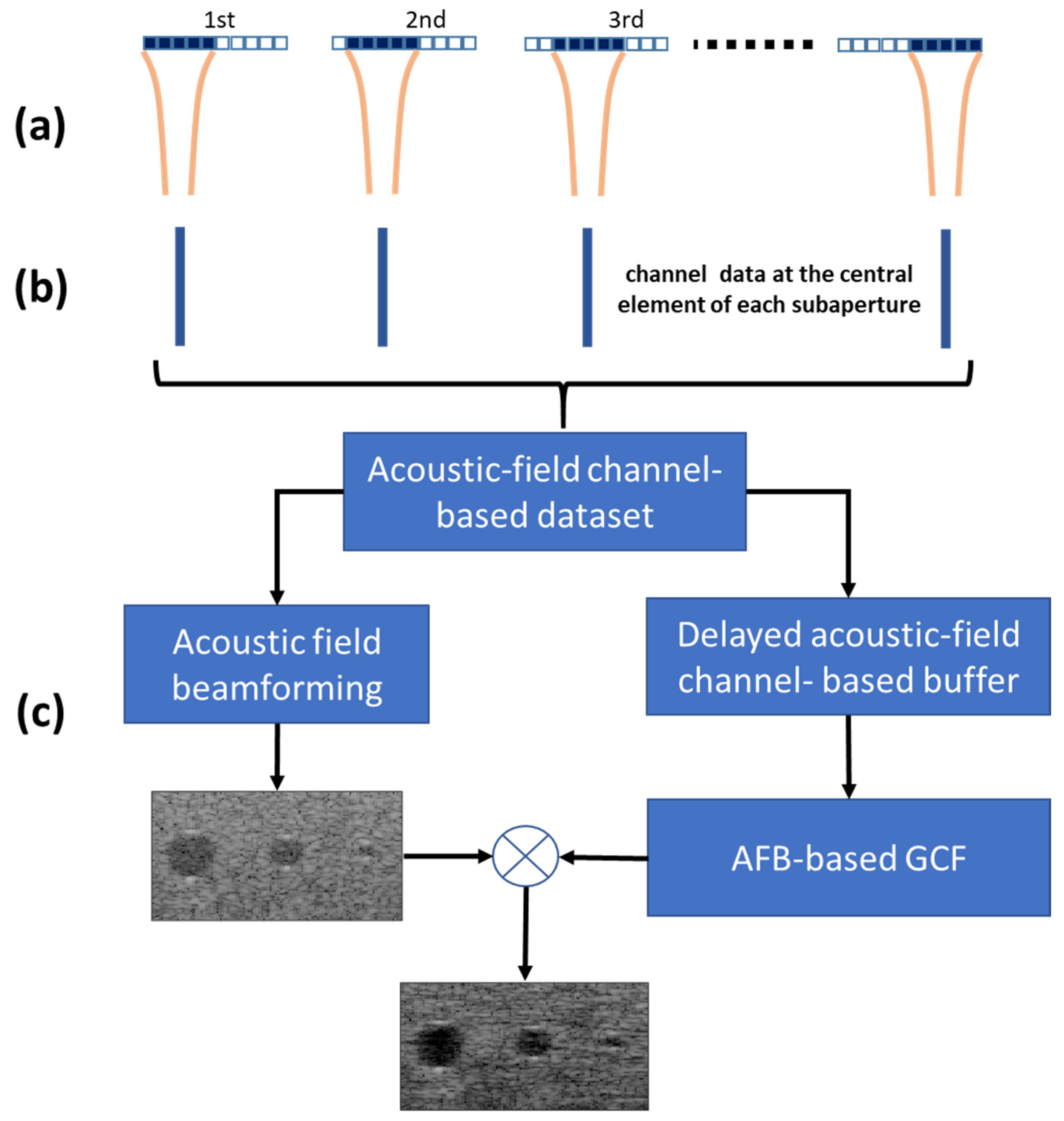
2.1. Acoustic Field Beamforming (AFB) Technology

Figure 1a shows the ultrasound transducer array including the M transducer elements with five elements used for transmitting ultrasonic signals for each scan line. Subsequently, the central element of each subaperture (i.e., only a single element) was used to receive the reflected ultrasound signal for each scan line, as shown in Figure 1b. As seen in Figure 1a,b, the transmission pattern was repeated through the transducer array, and then every received reflected ultrasound signal from each scan was collected to comprise an acoustic-field channel-based data set. Figure 1c shows a system block diagram of the GCF technique applied to AFB.
Based on the theory of the AFB technique [20], the receive delay time τ could be expressed as follows:
τ = 2 R c
where R represents the distance between the central element and the point of ultrasound image, and c is the velocity of sound. In Figure 1c, the AFB is implemented as the following sum:
S AFB ( t ) = j = i N 2 j = i + N 2 S j ( t τ )
where Sj represents the received ultrasound signal by the j-th element in the acoustic-field channel-based data set and i is the i-th line of AFB imaging.
The sum in the Equation (2) includes the number N of elements in the acoustic-field channel-based data set, which is selected as:
N = Z k 3 × Z f × M
where M represents the number of transducer elements, Zk represents the k-th point depth of the AFB image, and Zf represents the transmit focusing depth.

2.2. AFB-Based Generalized Coherence Factor (GCF) Technology

In this study, we extend the GCF weighting method previously proposed for adaptive beamforming to AFB technique.
In Figure 1c, the AFB-based GCF weighting is deduced from the spatial frequency of the delayed acoustic-field channel-based buffer, which is the received data from the single element of the transducer from each scan after the focusing delays of the AFB technique are applied before beam summation.
The N-point discrete Fourier transform of the delayed acoustic-field channel-based data along the line of AFB imaging can be expressed as:
p ( k , t ) = n = i N 2 n = i + N 2 S d e l a y e d ( n , t ) e j 2 π n k N
where Sdelayed (n, t) is the delayed signal of the n-th line of AFB imaging, N is the number of elements in the acoustic-field channel-based data set, and k is the spatial frequency index (i.e., k = −N/2, −N/2 + 1,…, N/2). Furthermore, AFB-based GCF is defined by dividing the energy from the low-frequency area by the total spatial spectral energy of the delayed acoustic-field channel-based data, used to measure the signal coherence. Thus, AFB-based GCF could be expressed as:
AFB - based   GCF ( t ) = energy   from   low - frequency   area total   energy = k = M 0 k = M 0 | p ( k , t ) | 2 k = N / 2 k = N / 2 | p ( k , t ) | 2
Note that the low-spatial-frequency area is specified by M0, which is a cutoff frequency in the spatial frequency index. M0 = 0 means that the low-frequency area used to estimate AFB-based GCF is restricted to direct current only.

2.3. Point and Cyst Target Simulations

We used the Field II program to simulate ultrasound images of five-point targets and five cysts [35,36]. Five points were located at depths from 10 to 50 mm and each interval is 10 mm. In addition, five anechoic cysts with diameters of 5 mm were centered at depths from 10 to 50 mm and each interval was 10 mm. The ultrasound system simulation was based on a 128-element linear array with a 5-MHz center frequency and a bandwidth of 71%, with a pitch = 0.307 mm. The speed of sound was 1540 m/s. Moreover, white Gaussian noise was added to the raw channel data to estimate the signal-to-noise ratio (SNR) for evaluating the performance of the proposed method. Here, the white Gaussian noise was at the 40 dB level below the peak signal of the point target, and SNR was defined as the ratio between the peak signal of the point target and the root mean squared background noise.
According to a previous study, five transmit elements and only single receive element can provide the best image quality using the AFB technique [20]. Thus, we compared the simulation results of nine methods with 16 Tx/16 Rx DAS, 32 Tx/32 Rx DAS, 64 Tx/64 Rx DAS, 3 Tx/1 Rx AFB, 5 Tx/1 Rx AFB, 7 Tx/1 Rx AFB, 3 Tx/1 Rx GCF, 5 Tx/1 Rx GCF, and 7 Tx/1 Rx GCF. The 16 Tx/16 Rx DAS meant that 16 transmit channels and sixteen receive channels based on a linear scan would be used to reconstruct an ultrasound image using the DAS method. In this study, the depth of transmit focus was fixed at 30 mm, with dynamic receive focusing using the DAS method. The 5 Tx/1 Rx AFB meant that five transmit channels and one receive channel based on a linear scan were used to reconstruct an ultrasound image by the AFB technique. Here, in the AFB technique, the depth of transmit focus was fixed at 30 mm. In addition, the 5 Tx/1 Rx GCF means that using the acoustic-field channel-based data set of 5 Tx/1 Rx AFB to reconstruct an ultrasound image by the AFB-based GCF weighting technique.

2.4. Experimental Setup

In the experimental method, we used a Gammex Ultrasound 1430 LE Phantom and a Verasonics research ultrasound platform to investigate the efficacy of the AFB-based GCF weighting method on sidelobe reduction in AFB imaging. The experimental images were acquired with 16 Tx/16 Rx DAS, 32 Tx/32 Rx DAS, 64 Tx/64 Rx DAS, 3 Tx/1 Rx AFB, 5 Tx/1 Rx AFB, 7 Tx/1 Rx AFB, 3 Tx/1 Rx GCF, 5 Tx/1 Rx GCF, and 7 Tx/1 Rx GCF. The parameters of the experiments were a 128-element, 0.3-mm pitch linear array, and a central frequency of 5 MHz. In the experimental data using the DAS method, the depth of transmit focus was fixed at 30 mm with receive dynamic focusing. In addition, the depth of transmit focus was fixed at 30 mm and single receive element was used by AFB technology.

2.5. In Vivo Carotid Artery Data

In this study, we obtained the experimental carotid artery data from the Ultrasonic Lab of the Industrial Technology Research Institute [20]. In vivo carotid artery data were obtained from a healthy volunteer (male, 40 years old) [37]. A Verasonics ultrasound system was equipped with an L7-4 ATL linear array transducer with 128 elements to acquire data. The parameters of the experiments were 5 MHz center frequency, 67% bandwidth, and a pitch of 0.3 mm [38,39]. The carotid artery in vivo results with 16 Tx/16 Rx DAS, 32 Tx/32 Rx DAS, 5 Tx/1 Rx AFB, 7 Tx/1 Rx AFB, 5 Tx/1 Rx GCF, and 7 Tx/1 Rx GCF were acquired. In the DAS method, the depth of transmit focus was fixed at 20 mm with dynamic receive focusing. In AFB technology, the depth of transmit focus was fixed at 20 mm and only a single receive element was used.

2.6. Image Quality Estimation

In this study, the lateral point target widths measured at −6 dB to act as a spatial resolution metric in the lateral direction [20]. The CR metric was measured to quantitatively evaluate the quality of ultrasound images under cyst targets. The CR was defined as difference of mean values of the kernels between the cyst and speckle zones in decibel (dB) scale. That is,
CR = | μ c μ s |
where μc is the mean value in dB within the cyst and μs is the mean value of speckle region in dB scale. In addition, the CNR was defined as the ratio of the CR value to the variance of the speckle area and cyst zone [40,41,42,43]. CNR can be expressed as follows,
CNR = CR σ c 2 + σ s 2
where σc represents the standard deviation, which is abbreviated STD, of the intensity within the cyst in dB scale, and σs represents the STD of the intensity at the speckle zone in dB scale. In addition, σs represents the speckle noise.

2.7. Selection of M0

Figure 2a shows the simulated B-mode images with an anechoic cyst at a depth of 30 mm using 5 Tx/1 Rx AFB. Figure 2b–i represents the simulated ultrasound images with an anechoic cyst using 5 Tx/1 Rx GCF when M0 was set from 8 to 24, respectively. We used Figure 2 to determine the low-energy spatial frequency region, that is, M0, for the AFB-based GCF estimation. Here, the STD of the intensity at the speckle zone was used to estimate speckle noise. In addition, CR and CNR were estimated using the speckle and the cyst zones. The outer dashed red box represents the speckle zone and the inner red box represents the cyst zone, as shown in Figure 2e.
Figure 3 shows the CR, STD, and CNR values of the anechoic cyst images using the AFB-based GCF technique as a function of M0. Figure 3 shows that the CR and STD decrease when the M0 value increases. In addition, Figure 3 shows that the best CNR could be achieved using the AFB-based GCF weighting technique when M0 is equal to 16. The results of CNR can be taken into consideration when choosing a proper M0. Thus, we chose M0 = 16 for this study.

3. Results and Discussion

3.1. Point-Target Simulations

Figure 4 shows the five-point targets simulation results over a 65 dB dynamic range with the nine methods. In the Figure 4e, we used the red box of the background region to estimate the background noise level. Figure 5 shows the lateral profile of the projections of the third point target image in Figure 4. Table 1 lists the beam width at the −6-dB level of the beam profile in the lateral direction that represents spatial resolution and SNR at the five-point depth zones. Among the three kinds of DAS methods shown in Figure 4a–c, the lateral resolution of the third point, the transmit focusing zone, using the 64 Tx/64 Rx DAS method was the best. The resolution and SNR of 64 Tx/64 Rx DAS was better than those of 16 Tx/16 Rx DAS and 32 Tx/32 Rx DAS due to a higher f-number from a larger array aperture, as listed in Table 1. Among the results of the three kinds of AFB technique, as shown in Figure 4d–f, we observed that the best lateral resolution and SNR could be achieved when using 5 Tx/1 Rx AFB, as shown in Table 1. At the third point depth zone, the lateral spatial resolutions and SNRs were similar between 5 Tx/1 Rx AFB and 64 Tx/64 Rx DAS. At the other points of depth zones (i.e., 10, 20, 40, and 50 mm), the results of lateral resolutions and SNRs with 5 Tx/1 Rx AFB were better than those with 64 Tx/64 Rx DAS. Among the results of the three kinds of the AFB-based GCF method, as shown in Figure 4g–i, we found that the results of the lateral resolutions were similar to those using the AFB technique. The SNR of AFB imaging is higher about 5–10 dB than that of DAS imaging and the SNR of AFB imaging after AFB-based GCF weighting is improved further by 8–12 dB, as listed in Table 1. In addition, Figure 5 shows the sidelobe level of the nine methods at the lateral position of −4 mm in the projected lateral profile of the third point at a depth of 30 mm. As seen in Figure 5, the AFB-based GCF technique provides a lower sidelobe level as compared with the DAS method and the AFB technique. Therefore, the AFB-based GCF technique can further suppress the sidelobe level using the AFB technique.

3.2. Anechoic Cyst Simulation

We used anechoic cyst simulation of ultrasound B-mode imaging from the diffuse scattered fields to verify the performance of the AFB-based GCF technique. Figure 6a–i represents the five anechoic cysts simulation results with the nine methods. The depths at five cysts are from 10 to 50 mm and each interval is 10 mm. The horizontal axis is the lateral distance, and the vertical axis is the depth in millimeters. Here, the CR, STD, and CNR were calculated from the cyst and the speckle zones. The inner red box represents the cyst zone and the outer dashed red box represents the speckle zone as shown in Figure 6d. The STD represents the speckle noise. The CR, STD, and CNR of the 2nd, 3rd, and 4th anechoic cyst images beamformed shown in Figure 6 with nine different methods are listed in Table 2. For the results of the three kinds of DAS methods shown in Figure 6a–c, at the third cyst zone (transmit focus zone) of the image, 64 Tx/64 Rx DAS provided the best CR and CNR. Among the results of the three kinds of AFB technique shown in Figure 6d–f, 5 Tx/1 Rx AFB provided the best CNR in the image quality metrics. In Figure 6, the AFB-based GCF technique improved the CR and CNR of the B-mode images using the AFB technique. The AFB-based GCF technique provided a clearer view of the cyst and surrounding structures than the AFB technique did. However, according to the STDs listed in Table 2, the speckle noises were increased after the AFB-based GCF weighting. Overall, the image quality in terms of CR and CNR was still improved for AFB-based GCF weighted images.

3.3. Experimental Results

Figure 7 shows the experimental B-mode images of the phantom experiments using the nine methods. Figure 7 also displays the experimental images on a dynamic range of 80 dB. Table 3 lists the CR, STD, and CNR of the experimental phantom images beamformed using nine methods, as shown in Figure 7. The outer dashed red box represents the speckle zone and the inner red box represents the cyst zone in Figure 7f. For the DAS method and AFB technique, the STD values that represent speckle noise are 5.26 dB, 5.47 dB, 5.6 dB, 5.34 dB, 5.32 dB, and 5.01 dB, as listed in Table 3. However, after AFB-based GCF weighting, the STD values were increased. The AFB-based GCF technique improved the CR and CNR of the experimental phantom images using the AFB technique.

3.4. In Vivo Carotid Artery

Figure 8 shows the carotid artery in vivo results using six methods. Table 4 lists the CR, STD, and CNR of the images using the six methods. The AFB-based GCF technique improved the CR and CNR of the in vivo images with the AFB technique. The in vivo testing demonstrates that the AFB-based GCF method can still work in in vivo conditions.

3.5. Discussion

In AFB-based GCF technique, the tradeoff of cutoff frequency M0 selection is between CR and STD. Herein, M0 of 16 is the best option for this study to obtain the best CNR. However, different ultrasound imaging parameters such as transmit frequencies, receive bandwidths, and aperture shapes would generate different shaped beam patterns, which affect the selection of M0 [34].
Based on the results of point-target simulations in Section 3.1, we found the original lateral resolution of AFB imaging would be maintained after AFB-based GCF weighting. Moreover, because the background noises of the AFB image can be further reduced after AFB-based GCF weighting, the SNR was further improved, as shown in Table 1. In addition, at the lateral position of −4 mm in Figure 5, the AFB-based GCF weighting can suppress the sidelobe of AFB imaging by 20 dB. The results of anechoic cyst simulation are consistent with experimental results in Section 3.2 and Section 3.3. After AFB-based GCF weighting, the image quality in terms of CRs and CNRs of AFB imaging were improved. In addition, Table 2 and Table 3 show that the speckle noise was similar using the DAS method and AFB technique. However, after AFB-based GCF weighting, the speckle noises were increased. The spatiotemporally smoothed coherence factor (STSCF) technique can be applied to the AFB-based GCF to reduce speckle-noise increase in future work [42].
Moreover, AFB-based GCF is estimated using Fourier transform from the delayed acoustic-field channel-based data for every imaging point which results in large computational complexity. To address this issue of GCF computational complexity, an autocorrelation-based GCF method has been proposed to estimate the GCF value [44]. The estimation of the GCF value from real signals is also proposed to lower computational complexity [45].

4. Conclusions

The use of the AFB technique has been proposed for handheld ultrasound to reduce electricity consumption and avoid battery and unwanted heat issues. In this study, our proposed AFB-based GCF technique is integrated in the AFB method to improve the image quality. In this work, the simulation data, experimental results, and in vivo testing verified the efficacy of our proposed AFB-based GCF technique. In addition, STSCF could be applied to the AFB-based GCF technique to improve the speckle the pattern.

Author Contributions

Conceptualization, C.-L.H. and M.-L.L.; methodology, I.-C.C. and P.-Z.S.; software, C.-L.H. and B.H.; validation, Z.-S.L. and C.-W.L.; simulation, C.-L.H.; formal analysis, M.-L.L.; investigation, C.-J.L. and H.-H.C.; writing—original draft preparation, all authors; writing—review and editing, all authors. All authors have read and agreed to the published version of the manuscript.

Funding

This research was funded by the Industrial Technology Research Institute under Grant No. M365EH1200 and M365EH1210.

Institutional Review Board Statement

Not applicable.

Informed Consent Statement

Not applicable.

Data Availability Statement

Data can be made available upon request.

Conflicts of Interest

The authors declare no conflict of interest.

References

  1. Yanikoglu, F.; Avci, H.; Celik, Z.C.; Tagtekin, D. Diagnostic performance of ICDAS II, FluoreCam and ultrasound for flat surface caries with different depths. Ultrasound Med. Biol. 2020, 46, 1755–1760. [Google Scholar] [CrossRef] [PubMed]
  2. Schapher, M.; Goncalves, M.; Mantsopoulos, K.; Iro, H.; Koch, M. Transoral ultrasound in the diagnosis of obstructive salivary gland pathologies. Ultrasound Med. Biol. 2019, 45, 2338–2348. [Google Scholar] [CrossRef]
  3. Moore, C.L.; Copel, J.A. Point-of-care ultrasonography. N. Engl. J. Med. 2011, 364, 749–757. [Google Scholar] [CrossRef] [Green Version]
  4. Kendall, J.L.; Hoffenberg, S.R.; Smith, R.S. History of emergency and critical care ultrasound: The evolution of a new imaging paradigm. Crit. Care Med. 2007, 35, S126–S130. [Google Scholar] [CrossRef] [PubMed]
  5. Cosby, K.S.; Kendall, J.L. Practical Guide to Emergency Ultrasound; Lippincott Williams & Wilkins: Philadelphia, PA, USA, 2006. [Google Scholar]
  6. Mayron, R.; Gaudio, F.E.; Plummer, D.; Asinger, R.; Elsperger, J. Echocardiography performed by emergency physicians: Impact on diagnosis and therapy. Ann. Emerg. Med. 1988, 17, 150–154. [Google Scholar] [CrossRef]
  7. Nelson, B.P.; Narula, J. How relevant is point-of-care ultrasound in LMIC? Glob. Heart 2013, 8, 287–288. [Google Scholar] [CrossRef] [PubMed]
  8. Daniels, J.M.; Hoppmann, R.A. Practical Point-of-Care Medical Ultrasound; Springer International Publishing: Cham, Switzerland, 2016. [Google Scholar]
  9. Wagner, M.S.; Garcia, K.; Martin, D.S. Point-of-care ultrasound in aerospace medicine: Known and potential applications. Aviat. Space Environ. Med. 2014, 85, 730–739. [Google Scholar] [CrossRef]
  10. Hwang, J.J.; Quistgaard, J.; Souquet, J.; Crum, L.A. Portable ultrasound device for battlefield trauma. In Proceedings of the 1998 IEEE Ultrasonics Symposium, Sendai, Japan, 5–8 October 1998; Volume 2, pp. 1663–1667. [Google Scholar]
  11. Nelson, B.P.; Chason, K. Use of ultrasound by emergency medical services: A review. Int. J. Emerg. Med. 2008, 1, 253–259. [Google Scholar] [CrossRef] [Green Version]
  12. Thompson, M.R. The Future of Portable Ultrasound: Business Strategies for Survival. Ph.D. Thesis, Massachusetts Institute of Technology, Cambridge, MA, USA, 2010. [Google Scholar]
  13. Rykkje, A.; Carlsen, J.F.; Nielsen, M.B. Hand-held ultrasound devices compared with high-end ultrasound systems: A systematic review. Diagnostics 2019, 9, 61. [Google Scholar] [CrossRef] [Green Version]
  14. Becker, D.M.; Tafoya, C.A.; Becker, S.L.; Kruger, G.H.; Tafoya, M.J.; Becker, T.K. The use of portable ultrasound devices in low-and middle-income countries: A systematic review of the literature. Trop. Med. Int. Health 2016, 21, 294–311. [Google Scholar] [CrossRef]
  15. Reeder, R.; Petersen, C. 8-Channel, 12-Bit, 10-MSPS to 50-MSPS Front End: The AD9271–A Revolutionary Solution for Portable Ultrasound. Analog. Dialogue 2007, 41, 3. [Google Scholar]
  16. Brunner, E. How ultrasound system considerations influence front-end component choice. Analog. Dialogue 2002, 36, 1–4. [Google Scholar]
  17. Szabo, T.L. Diagnostic Ultrasound Imaging: Inside Out; Academic Press: Cambridge, MA, USA, 2004. [Google Scholar]
  18. Qiu, W.; Yu, Y.; Tsang, F.K.; Sun, L. A multifunctional, reconfigurable pulse generator for high-frequency ultrasound imaging. IEEE Trans. Ultrason. Ferroelectr. Freq. Control 2012, 59, 1558–1567. [Google Scholar] [PubMed]
  19. Choi, H. Stacked transistor bias circuit of class-b amplifier for portable ultrasound systems. Sensors 2019, 19, 5252. [Google Scholar] [CrossRef] [PubMed] [Green Version]
  20. Hu, C.L.; Wu, G.Z.; Chang, C.C.; Li, M.L. Acoustic-Field Beamforming for Low-Power Portable Ultrasound. Ultrason. Imaging 2021, 43, 175–185. [Google Scholar] [CrossRef]
  21. Perrot, V.; Polichetti, M.; Varray, F.; Garcia, D. So you think you can DAS? A viewpoint on delay-and-sum beamforming. Ultrasonics 2021, 111, 106309. [Google Scholar] [CrossRef] [PubMed]
  22. Paul, S.; Thomas, A.; Mayanglambam, S.S. Improvement of Delay and Sum beamforming photoacoustic imaging based on delay-multiply-sum-to-standard-deviation-factor. Int. Soc. Opt. Photonics 2021, 11642, 116423D. [Google Scholar]
  23. Steinberg, B.D. Digital beamforming in ultrasound. IEEE Trans. Ultrason. Ferroelectr. Freq. Control 1992, 39, 716–721. [Google Scholar] [CrossRef] [PubMed]
  24. Cohen, R.; Eldar, Y.C. Sparse convolutional beamforming for ultrasound imaging. IEEE Trans. Ultrason. Ferroelectr. Freq. Control 2018, 65, 2390–2406. [Google Scholar] [CrossRef] [PubMed] [Green Version]
  25. Hewener, H.; Risser, C.; Brausch, L.; Rohrer, T.; Tretbar, S. A mobile ultrasound system for majority detection. In Proceedings of the 2019 IEEE International Ultrasonics Symposium, Glasgow, UK, 6–9 October 2019; pp. 502–505. [Google Scholar]
  26. Alexander, J. Xilinx devices in portable ultrasound systems. WP378 (v1. 2). Available online: https://www.xilinx.com/support/documentation/white_papers/wp378-Xilinx-in-Portable-Ultrasound.pdf (accessed on 13 December 2021).
  27. Maxim, Datasheet MAX2082. Low-Power, High-Performance Octal Ultrasound Transceiver with Integrated AFE, Pulser, T/R Switch, and CWD Beamformer; Maxim Integrated Products: San Jose, CA, USA, 2014. [Google Scholar]
  28. Mallart, R.; Fink, M. Adaptive focusing in scattering media through sound-speed inhomogeneities: The van Cittert Zernike approach and focusing criterion. J. Acoust. Soc. Am. 1994, 96, 3721. [Google Scholar] [CrossRef]
  29. Rindal, O.M.H.; Austeng, A.; Torp, H.; Holm, S.; Rodriguez-Molares, A. The dynamic range of adaptive beamformers. In Proceedings of the 2016 IEEE International Ultrasonics Symposium, Tours, France, 18–21 September 2016; pp. 1–4. [Google Scholar]
  30. Hollman, K.W.; Rigby, K.W.; O’donnell, M. Coherence factor of speckle from a multi-row probe. In Proceedings of the 1999 IEEE Ultrasonics Symposium, Tahoe, NV, USA, 17–20 October 1999; Volume 2, pp. 1257–1260. [Google Scholar]
  31. Nilsen, C.I.C.; Holm, S. Wiener beamforming and the coherence factor in ultrasound imaging. IEEE Trans. Ultrason. Ferroelectr. Freq. Control 2010, 57, 1329–1346. [Google Scholar] [CrossRef]
  32. Camacho, J.; Parrilla, M.; Fritsch, C. Phase coherence imaging. IEEE Trans. Ultrason. Ferroelectr. Freq. Control 2009, 56, 958–974. [Google Scholar] [CrossRef] [PubMed]
  33. Li, M.L.; Li, P.C. A new adaptive imaging technique using generalized coherence factor. In Proceedings of the 2002 IEEE Ultrasonics Symposium, Munich, Germany, 8–11 October 2002; Volume 2, pp. 1627–1630. [Google Scholar]
  34. Li, P.C.; Li, M.L. Adaptive imaging using the generalized coherence factor. IEEE Trans. Ultrason. Ferroelectr. Freq. Control 2003, 50, 128–141. [Google Scholar]
  35. Jensen, J.A. Field: A program for simulating ultrasound systems. In Proceedings of the 10th Nordic-Baltic Conference on Biomedical Imaging, Tampere, Finland, 9–13 June 1996; Volume 4, pp. 351–353. [Google Scholar]
  36. Jensen, J.A.; Svendsen, N.B. Calculation of pressure fields from arbitrarily shaped, apodized, and excited ultrasound transducers. IEEE Trans. Ultrason. Ferroelectr. Freq. Control 1992, 39, 262–267. [Google Scholar] [CrossRef] [Green Version]
  37. Hu, C.L.; Cheng, I.C.; Huang, C.H.; Liao, Y.T.; Lin, W.-C.; Tsai, K.J.; Chi, C.H.; Chen, C.W.; Wu, C.H.; Lin, I.T.; et al. Dry Wearable Textile Electrodes for Portable Electrical Impedance Tomography. Sensors 2021, 21, 6789. [Google Scholar] [CrossRef] [PubMed]
  38. Saris, A.E.; Hansen, H.H.; Fekkes, S.; Nillesen, M.M.; Rutten, M.C.; de Korte, C.L. A comparison between compounding techniques using large beam-steered plane wave imaging for blood vector velocity imaging in a carotid artery model. IEEE Trans. Ultrason. Ferroelectr. Freq. Control 2016, 63, 1758–1771. [Google Scholar] [CrossRef] [PubMed]
  39. Liebgott, H.; Rodriguez-Molares, A.; Cervenansky, F.; Jensen, J.A.; Bernard, O. Plane-wave imaging challenge in medical ultrasound. In Proceedings of the 2016 IEEE International Ultrasonics Symposium, Tours, France, 18–21 September 2016; pp. 1–4. [Google Scholar]
  40. Smith, S.W.; Wagner, R.F. Ultrasond speckle size and lesion signal to noise ratio: Verification of theory. Ultrason. Imaging 1984, 6, 174–180. [Google Scholar] [CrossRef]
  41. Karaman, M.; Li, P.C.; O’Donnell, M. Synthetic aperture imaging for small scale systems. IEEE Trans. Ultrason. Ferroelectr. Freq. Control 1995, 42, 429–442. [Google Scholar] [CrossRef]
  42. Xu, M.; Yang, X.; Ding, M.; Yuchi, M. Spatio-temporally smoothed coherence factor for ultrasound imaging. IEEE Trans. Ultrason. Ferroelectr. Freq. Control 2014, 61, 182–190. [Google Scholar] [CrossRef]
  43. Santos, P.; Koriakina, N.; Chakraborty, B.; Pedrosa, J.; Petrescu, A.M.; Voigt, J.U.; D’hooge, J. Evaluation of coherence-based beamforming for B-mode and speckle tracking echocardiography. In Proceedings of the 2018 IEEE International Ultrasonics Symposium, Kobe, Japan, 22–25 October 2018; pp. 1–4. [Google Scholar]
  44. Shen, C.C.; Xing, Y.Q.; Jeng, G. Autocorrelation-based generalized coherence factor for low-complexity adaptive beamforming. Ultrasonics 2016, 72, 177–183. [Google Scholar] [CrossRef]
  45. Hisatsu, M.; Mori, S.; Arakawa, M.; Kanai, H. Generalized coherence factor estimated from real signals in ultrasound beamforming. J. Med. Ultrason. 2020, 47, 179–192. [Google Scholar] [CrossRef] [PubMed]
Figure 1. Schematic of the acoustic field beamforming (AFB)-based generalized coherence factor (GCF) method. (a) Repeat transmit pattern through the array. (b) Compose an acoustic-field channel-based data set. (c) The system block diagram for the AFB-based GCF technique.
Applsci 12 00560 g001
Figure 2. Images of an anechoic cyst over a 65-dB dynamic range. (a) 5 Tx/1 Rx AFB. (b) 5 Tx/1 Rx GCF with M0 = 8. (c) M0 = 10. (d) M0 = 12. (e) M0 = 14. (f) M0 = 16. (g) M0 = 18. (h) M0 = 20. (i) M0 = 22. (j) M0 = 24.
Applsci 12 00560 g002
Figure 3. Quantitative analysis of contrast ratio (CR), standard deviation (STD) and contrast-to-noise ratio (CNR) as a function of M0.
Applsci 12 00560 g003
Figure 4. Five-point targets simulation results of nine methods. (a) 16 Tx/16 Rx DAS. (b) 32 Tx/32 Rx DAS. (c) 64 Tx/64 Rx DAS. (d) 3 Tx/1 Rx AFB. (e) 5 Tx/1 Rx AFB. (f) 7 Tx/1 Rx AFB. (g) 3 Tx/1 Rx GCF. (h) 5 Tx/1 Rx GCF. (i) 7 Tx/1 Rx GCF.
Applsci 12 00560 g004
Figure 5. Beam profile in the lateral direction at the third point depth zone in Figure 4.
Applsci 12 00560 g005
Figure 6. Five anechoic cysts simulation results of nine methods. (a) 16 Tx/16 Rx DAS. (b) 32 Tx/32 Rx DAS. (c) 64 Tx/64 Rx DAS. (d) 3 Tx/1 Rx AFB. (e) 5 Tx/1 Rx AFB. (f) 7 Tx/1 Rx AFB. (g) 3 Tx/1 Rx GCF. (h) 5 Tx/1 Rx GCF. (i) 7 Tx/1 Rx GCF.
Applsci 12 00560 g006
Figure 7. Anechoic cysts experimental results of nine methods. (a) 16 Tx/16 Rx DAS. (b) 32 Tx/32 Rx DAS. (c) 64 Tx/64 Rx DAS. (d) 3 Tx/1 Rx AFB. (e) 5 Tx/1 Rx AFB. (f) 7 Tx/1 Rx AFB. (g) 3 Tx/1 Rx GCF. (h) 5 Tx/1 Rx GCF. (i) 7 Tx/1 Rx GCF.
Applsci 12 00560 g007
Figure 8. Carotid artery in vivo results. (a) 16 Tx/16 Rx DAS. (b) 32 Tx/32 Rx DAS. (c) 5 Tx/1 Rx AFB. (d) 7 Tx/1 Rx AFB. (e) 5 Tx/1 Rx GCF. (f) 7 Tx/1 Rx GCF.
Applsci 12 00560 g008
Table 1. Comparison of the beam widths at the −6-dB level of the lateral profile of projections representing the lateral spatial resolution and SNR at the five-point depth zones, as shown in Figure 4.
−6 dB (mm)16 Tx/16 Rx DAS32 Tx/32 Rx DAS64 Tx/64 Rx DAS3 Tx/1 Rx AFB5 Tx/1 Rx AFB7 Tx/1 Rx AFB3 Tx/1 Rx GCF5 Tx/1 Rx GCF7 Tx/1 Rx GCF
1st point (10 mm)1.121.291.640.620.670.960.620.660.96
2nd point (20 mm)1.491.051.380.670.541.20.680.551.21
3rd point (30 mm)2.541.110.580.820.591.650.840.611.68
4th point (40 mm)3.491.641.380.960.671.790.980.681.82
5th point (50 mm)6.183.83.21.261.422.061.281.432.08
SNR (dB)16 Tx/16 Rx DAS32 Tx/32 Rx DAS64 Tx/64 Rx DAS3 Tx/1 Rx AFB5 Tx/1 Rx AFB7 Tx/1 Rx AFB3 Tx/1 Rx GCF5 Tx/1 Rx GCF7 Tx/1 Rx GCF
1st point (10 mm)37.1638.5639.3748.548.2846.5760.0961.6757.72
2nd point (20 mm)44.8549.7849.8355.7254.5952.9268.0366.0762.59
3rd point (30 mm)47.6251.7156.3155.7456.5254.2567.3664.5564.33
4th point (40 mm)43.8245.5245.6154.1955.3754.0166.4465.6765.64
5th point (50 mm)42.6142.7643.7953.8655.1952.1263.9165.1663.51
Table 2. Contrast (CR), standard deviation (STD), and contrast-to-noise ratio (CNR) of the 2nd, 3rd, and the 4th cyst images acquired with nine methods, as shown in Figure 6.
CR (dB)16 Tx/16 Rx DAS32 Tx/32 Rx DAS64 Tx/64 Rx DAS3 Tx/1 Rx AFB5 Tx/1 Rx AFB7 Tx/1 Rx AFB3 Tx/1 Rx GCF5 Tx/1 Rx GCF7 Tx/1 Rx GCF
2nd cyst (20 mm)23.0228.2520.9210.5212.2215.1429.3432.4433.38
3rd cyst (30 mm)24.9230.6837.114.1416.3812.7536.1337.6530.73
4th cyst (40 mm)16.5626.420.6313.9111.1216.8328.3424.8930.97
STD (dB)16 Tx/16 Rx DAS32 Tx/32 Rx DAS64 Tx/64 Rx DAS3 Tx/1 Rx AFB5 Tx/1 Rx AFB7 Tx/1 Rx AFB3 Tx/1 Rx GCF5 Tx/1 Rx GCF7 Tx/1 Rx GCF
2nd cyst (20 mm)7.187.386.815.415.775.949.58.98.69
3rd cyst (30 mm)5.746.156.16.415.566.147.57.68.59
4th cyst (40 mm)6.756.736.926.15.715.549.28.68.59
CNR16 Tx/16 Rx DAS32 Tx/32 Rx DAS64 Tx/64 Rx DAS3 Tx/1 Rx AFB5 Tx/1 Rx AFB7 Tx/1 Rx AFB3 Tx/1 Rx GCF5 Tx/1 Rx GCF7 Tx/1 Rx GCF
2nd cyst (20 mm)2.462.942.961.292.211.462.312.562.64
3rd cyst (30 mm)2.963.623.921.432.322.212.963.352.9
4th cyst (40 mm)1.912.962.981.662.012.22.312.352.87
Table 3. Contrast (CR), standard deviation (STD), and contrast-to-noise ratio (CNR) of the images acquired using nine methods, as shown in Figure 7.
16 Tx/16 Rx DAS32 Tx/32 Rx DAS64 Tx/64 Rx DAS3 Tx/1 Rx AFB5 Tx/1 Rx AFB7 Tx/1 Rx AFB3 Tx/1 Rx GCF5 Tx/1 Rx GCF7 Tx/1 Rx GCF
CR (dB)20.4322.8523.2219.0219.2319.0633.4133.933.76
STD (dB)5.265.475.65.345.325.018.038.048.1
CNR2.672.9732.452.562.553.23.263.22
Table 4. Contrast (CR), standard deviation (STD), and contrast-to-noise ratio (CNR) of the images acquired using six methods, as shown in Figure 8.
16 Tx/16 Rx DAS32 Tx/32 Rx DAS5 Tx/1 Rx AFB7 Tx/1 Rx AFB5 Tx/1 Rx GCF7 Tx/1 Rx GCF
CR (dB)18.8620.119.7215.4434.7727.31
Std (dB)6.875.516.326.347.517.91
CNR2.012.322.231.862.522.02
Publisher’s Note: MDPI stays neutral with regard to jurisdictional claims in published maps and institutional affiliations.

