Abstract
This paper presents a novel parameter identification and uncertainty quantification method for flutter derivatives estimation of bridge decks. The proposed approach is based on free-decay vibration records of a sectional model in wind tunnel tests, which consists of parameter identification by a heuristic optimization algorithm in the sense of weighted least squares and uncertainty quantification by a bootstrap technique. The novel contributions of the method are on three fronts. Firstly, weighting factors associated with vertical and torsional motion in the objective function are determined more reasonably using an iterative procedure rather than preassigned. Secondly, flutter derivatives are identified using a hybrid heuristic and classical optimization method, which integrates a modified artificial bee colony algorithm with the Powell’s algorithm. Thirdly, a statistical bootstrap technique is used to quantify the uncertainties of flutter derivatives. The advantages of the proposed method with respect to other methods are faster and more accurate achievement of the global optimum, and refined uncertainty quantification in the identified flutter derivatives. The effectiveness and reliability of the proposed method are validated through noisy data of a numerically simulated thin plate and experimental data of a bridge deck sectional model.
1. Introduction
As one kind of flexible structures, long-span bridges tend to vibrate greatly under wind load. One of the most important wind-induced vibration phenomena is the flutter since it is tightly linked to the safety of bridges. The safety margin for flutter must be carefully evaluated during the design process. Although CFD and AI-based methods can predict the wind pressure and vibration response of structures [1,2,3], wind tunnel tests are still the main research tool for evaluating the wind resistance performance of structures and will last for a period in the future [4]. The sectional model test is a common method of wind tunnel testing. In sectional model tests, representative models of a bridge deck with aerodynamic and geometrical similarity are elastically suspended in the wind tunnel, and their behavior in the wind flow can be extrapolated to full scale.
For flutter studies, a semi-empirical model characterizing the motion-dependent self-excited forces was first introduced by Scanlan in the 1970s [5]. In this model, the self-excited forces are functions of the flow speed, vibration frequency, and state vector, while the coefficients in front of the state vector are called flutter derivatives because they are essentially the first partial derivatives of the self-excited forces with respect to the state vector. To estimate the flutter derivatives in Scanlan’s model, free decay vibration, forced vibration, or random vibration sectional model wind tunnel tests are usually performed. The free decay vibration method measures the bending-torsion coupled free vibration response of the sectional model under no wind and in wind flow, and then extracts the flutter derivatives from the free vibration response. The forced vibration method refers to the use of a special mechanical device to drive the model to do harmonic vibration with a controllable frequency and amplitude; directly measure the vibration signals, such as the aerodynamic force, acting on the model and displacement or acceleration of the model; and then directly perform spectral analysis or time-domain analysis on the measured aerodynamic force and vibration signals to obtain the flutter derivatives. Traditionally, flutter derivative identification is carried out in uniform flow, and the effect of turbulence is ignored. Turbulence will alter the flow pattern around the section, which will affect the identification of the flutter derivatives. The random vibration method is to identify the flutter derivatives of the bridge deck by sectional model wind tunnel test in the grid-generated turbulence field. Either traditional eight flutter derivatives related to vertical bending and torsional motion from a two-degree-of-freedom (2DOF) sectional model or 18 flutter derivatives including additional sway motion from a 3DOF model are obtained. Among these three kinds of flutter derivative extraction methods, the free-decay vibration approach is the simplest one; for this reason, it is widely adopted and will be the focus of the present work. This method was first proposed by Scanlan and Tomko [5], using first two SDOF free-decay tests to extract the direct derivatives (, , ) and then a coupled 2DOF free-decay test to extract cross-derivatives (, , ). Sarkar et al. [6] proposed a system identification procedure designed to estimate eight derivatives simultaneously by a single 2DOF free-decay test. Gu et al. [7] proposed the unifying least squares (ULS) method to extract flutter derivatives, where a unified error function combining vertical and torsional motion was employed. In order to balance the vertical and torsion signals, Ding et al. [8] were the first researchers who introduced weighting factors into the ULS method for flutter derivative identification. Later, Li et al. [9] proposed the weighting ensemble least-square method (WELS) to extract flutter derivatives of bridge decks. Bartoli et al. [10] modified the ULS method by introducing proper weighting factors in the unified error function and enhancing the iterative solving procedure. The iterative scheme in the ULS was also enhanced by Xu et al. [11] using an improved stochastic search algorithm.
Most of the methods mentioned above are based on least squares. The flutter derivatives are extracted by minimizing the residual between measured signals and predicted responses. In these methods, the parameters are identified from the residuals related to vertical bending and torsional motion separately [5], or the sum of them without or with weighting factors [7,9,10]. By utilizing weighting factors in the objective function, the accuracy of the identification results is improved. However, the weighting factors used in the previous methods are preassigned, which may not be optimal. In contrast, in this paper, the weighting factors are optimized using an iterative procedure.
Generally, the flutter derivatives are extracted by solving an optimization problem, in which a good initial guess of the parameters is usually required, so that difficulties may arise to obtain a sound result when a poor initial value is used. Indeed, some researchers used the Modified Ibrahim Time Domain (MITD) approach [6,7] or the covariance block-Hankel matrix (CBHM) method [12,13] to determine the initial values of system parameters when identifying flutter derivatives of bridge decks. The results may not be accurate enough but are good enough to be the initial values. However, an extra step is required to determine the initial values in these methods. Therefore, methodologies based on heuristic search algorithms without initial values can be employed for this purpose. Several heuristic stochastic algorithms for global optimization have been developed in recent years, such as particle swarm optimization, harmony search algorithm, ant colony optimization, firefly algorithm, differential evolution algorithm, and gravitational search algorithm, etc. Besides the above-mentioned algorithms, in 2005, Karaboga [14] proposed a novel swarm intelligence algorithm, i.e., the artificial bee colony (ABC) algorithm, to solve complex numerical optimization problems. ABC is a heuristic optimization algorithm with the advantage of simple structure, convenient implementation, and good stability. For a good optimization algorithm, two search capabilities of exploitation and exploration need to be balanced. Exploitation is the behavior of probing a local region of the search space by fine-tuning, with the hope of improving a promising solution that we already have at hand. Exploration is the behavior leading to disengagement from the current solution by probing a larger search space for alternatives, with the hope of finding other promising and needing to be further refined solutions. However, the standard ABC algorithm is strong in exploration but weak in exploitation, which has greatly affected its performance. In truth, it is a critical issue for such a kind of heuristic search algorithm to keep a proper balance between the exploration and exploitation. Aiming at these problems, this paper introduces a modified ABC algorithm with Powell’s method (MABC-Powell) to solve the optimization problem, where the standard ABC is enhanced by several modifications [15,16,17,18].
It is noted that only a single optimal estimate of flutter derivatives can be made for one set of test data for most of the methods, and repeated tests for wind tunnel tests are only limited to some cases [19]. Moreover, due to the effects of flow turbulence, measurement noise, and mathematical model error, the estimation of flutter derivatives shows dispersed results in repeated experiments. Subsequently, if mishandled, the inherent uncertainty can lead to estimation errors. Uncertainty quantification is crucial to flutter reliability analysis [19,20,21,22,23] and reliability-based optimum design [24,25,26] of bridges. In order to properly quantify the uncertainties in the identified flutter derivatives, a statistical tool termed as bootstrap is proposed to determine the statistical characteristics of flutter derivatives [27].
In this study, an enhanced identification method of flutter derivatives of bridge decks is proposed. The proposed method has new improvements in the following three aspects: (1) the weighting factors are optimized in an iterative procedure; (2) an improved heuristic algorithm termed MABC-Powell is proposed for flutter derivatives identification; and (3) a bootstrap scheme is proposed for parameter uncertainty quantification. The proposed method is validated with simulated data of a thin plate and experimental data of a bridge deck.
2. Optimization Formulation of Flutter Derivatives Identification
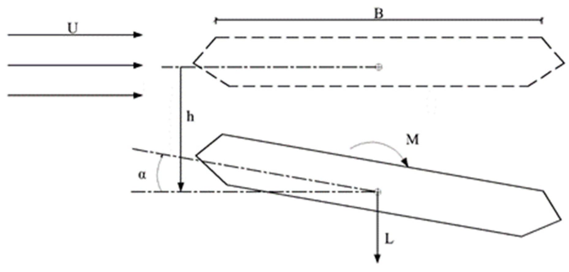
According to Scanlan’s model for flutter analysis, a 2DOF linear oscillator representing the bridge deck section vibrating in vertical displacement h(t) and torsional angle α(t) is shown in Figure 1. The equations of motion can be written as follows:
where m and I are the mass and mass moment of inertia per unit length; and are the circular frequencies of the vertical bending and torsional modes; and are the damping ratios of the vertical bending and torsional modes; and are the lift and pitching moment per unit length. Generally, the terms of the lift and pitching moment on the right-hand side involve three components of mean, buffeting, and self-excited forces; nevertheless, for free vibration tests, only the self-excited forces are retained since the motion is dominated by free decaying vibration around a mean position and thus the load due to signature turbulence can be neglected. The self-excited forces and can be expressed in Scanlan’s form as follows:
where ρ is the air density, and (i = 1, 2, 3, 4) are the flutter derivatives, B is the deck width, U is the mean wind velocity, and K = Bω/U is the reduced frequency of oscillation.
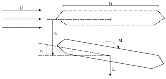
Figure 1.
Bridge deck section oscillating in two-dimensional smooth flow.
Substituting Equations (3) and (4) into Equations (1) and (2), respectively, yield:
where , , , , , , , . Rewriting Equations (5) and (6) in matrix form, yields:
where x = [h, α]T, , . Using a state vector , Equation (7) can be rewritten in state-space form as follows:
where A = [O, E; −K, −C], O is a 2 × 2 zero matrix and E is a 2 × 2 identity matrix. The flutter derivatives are involved in matrix A, and the free vibration response can be obtained by solving Equation (8). Neglecting the aerodynamic damping and stiffness in still air, the aerodynamic matrices are obtained by comparing the measured matrices in wind flow and in still air.
The predicted free-vibration time histories of vertical displacement h(t) and torsional angle α(t) can be expressed as follows:
where the four parameters ai and bi are determined by the complex conjugate eigenvalues of matrix A in Equation (8), , ; the other eight parameters ci, di, ei, and fi are determined by the initial conditions.
Let the data length of one set of measured vertical displacement signal and torsional angle signal be N, the error vectors between measurements and predictions can be expressed as follows:
If the tests are repeated for M times at the same wind speed, and then M sets of free-vibration records are available, the total residual error function takes the form:
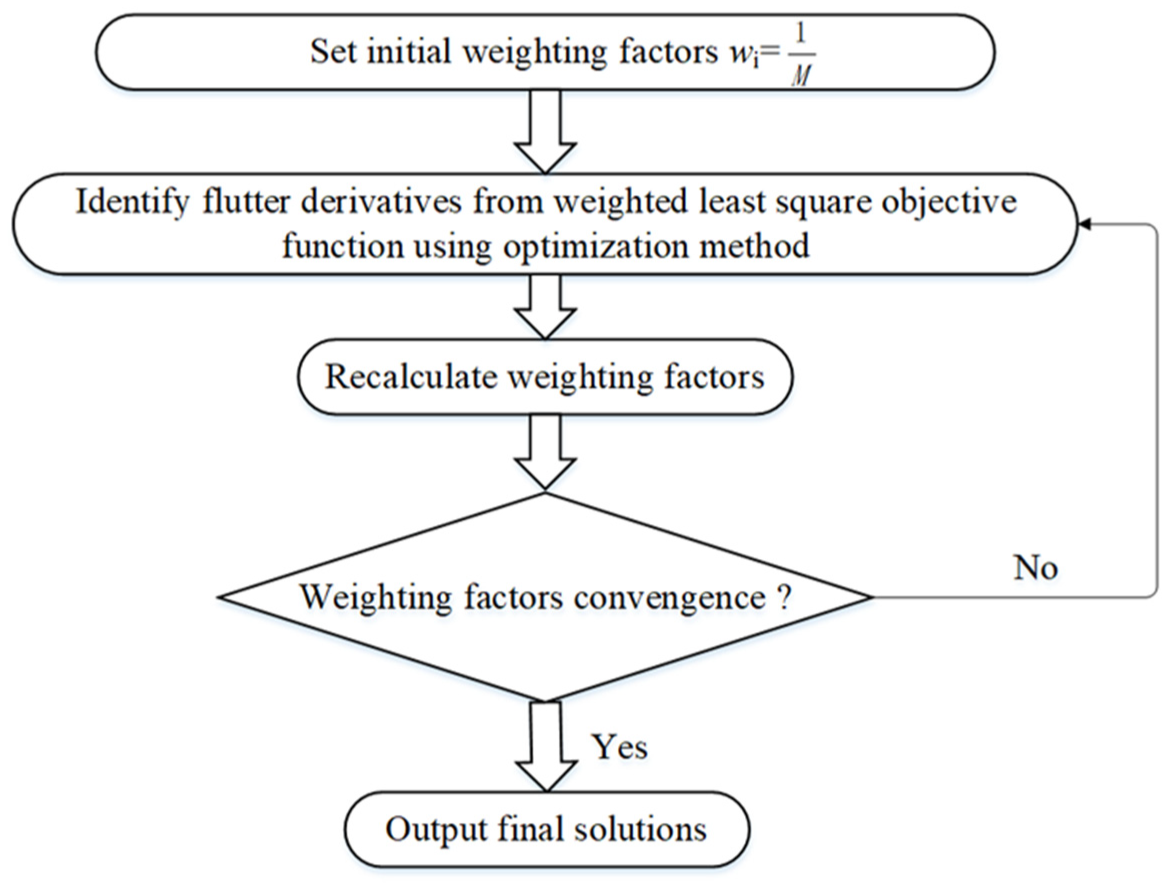
where and are the weighting factors for vertical bending and torsional motion of the mth free-vibration records, respectively. In the previous methods, the weighting factors were almost preassigned by experience and intuition. For example, in the weighted ensemble least squares method [9], the weighting factors are chosen as the ratio of maximum of root-mean-square (RMS) values to the corresponding RMS of the free-vibration time history so as to balance the relative errors between them. In the MULS method [10], the weighting factors are chosen based on the transformation of torsional angles from vertical displacements of the section leading edge. Herein, instead of using preassigned weighting factors, we propose using optimal weighting factors, which are determined iteratively. Christodoulou and Papadimitriou carried out a strict theoretical derivation of the optimal weighting factors in the weighted least squares method [28]. They showed that the optimal weighting factor of a residual group in the objective function is asymptotically, for a large number of measured data, inversely proportional to the residual group value of the optimal parameters. The general weighted least squares objective function can be written as:
where is a function of unknown parameters θ related to a specific group of residuals, and is the associated weighting factor. The optimal value of in Equation (14) is given by:
where is the estimated optimal value of θ with regards to minimization of Equation (14), and is a scale parameter representing the ratio of data volume in each residual group. Let Nm denote the number of data in the mth group of data, then the total number , , satisfying . However, the optimal value given in Equation (15) is a function of the optimal parameter vector to be determined, which cannot be obtained directly and can only be solved iteratively. The initial values of can be set to 1/M. Solving Equation (14) by using an optimization method, a temporary optimal value is obtained, and then the new weight factor is recalculated by using Equation (15). This procedure is repeated several times until a convergence criterion is satisfied. This procedure is depicted in Figure 2. The optimization method utilized is described in the next section.
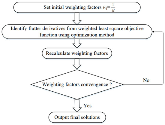
Figure 2.
Flowchart of flutter derivatives identification by the optimized weighted least square method.
3. Artificial Bee Colony Algorithm
3.1. Standard ABC Algorithm
Inspired by bees’ nectar collecting behavior in nature, the optimization process of the ABC algorithm is based on the mechanism of searching for the best nectar source. In the ABC algorithm, the location of a nectar source stands for a possible solution to the optimization problem, and the amount of nectar represents the fitness of the corresponding solution. In applying the ABC algorithm to the flutter derivatives identification problem, finding the possible “best” nectar source is equivalent to finding the optimal solution corresponding to Equation (13).
In the ABC algorithm, the artificial bee swarm consists of three types of bees: employed bees, onlooker bees, and scout bees. The number of solutions in the population is equal to half of the total bee number: the first half of the swarm are employed bees, while the second half are the onlooker bees. The algorithm begins with a population of size SN (X1, X2, …, XSN), which are randomly sampled from the parameter space, and each cycle of the search consists of three steps: employed bee phase, onlooker bee phase, and scout bee phase.
In the employed bee phase, a new nectar source Vi is produced based on its preceding position Xi by a solution search equation as follows. In vector components, this can be written as:
where k ∈ {1, 2, …, SN} and j ∈ {1, 2, …, D} are randomly chosen indexes, and D is the number of optimization parameters; k has to be different from i, and is a random number in the range [−1, 1]. If Vi is better than Xi, then Xi is replaced with Vi; otherwise, the old nectar source Xi is retained.
In the onlooker bee phase, an onlooker bee chooses a nectar source depending on the probability value pi associated with the nectar amount of that nectar source:
where fiti is the fitness value of solution i. The fitness value is calculated as , and J is the value of total residual error function in Equation (13).
Finally, in the scout bee phase, a nectar source is considered depleted and discarded when it remains unchanged for a predefined limit number of times. If the nectar source Xi is abandoned, then a new nectar source will be chosen by the scout bee at random, as shown below:
where rand is a random number uniformly distributed within the range [0,1], and [,] is the boundary constraint for the jth variable.
The pseudo-code of the standard ABC algorithm is given in Appendix A (Algorithm A1).
3.2. Modified ABC Algorithm with Powell’s Method
Optimization algorithms have two behaviors: exploration and exploitation. Exploration is the behavior of generating candidate solutions that are not adjacent to the current solution to avoid local optimality, while exploitation is the behavior of searching for a better solution in the neighborhood of the current solution. As a swarm intelligence algorithm, the standard ABC algorithm is strong at exploration but weak at exploitation. To tackle this problem, three modifications of the standard ABC algorithm are proposed to improve its convergence and provide a good trade-off between exploration and exploitation. These modifications involve solution updating with a best neighbor-guided approach and a decaying factor, enhanced local search with Powell’s method, and Scout solution rebirth with Gaussian mutation.
3.2.1. Modification I: Solution Updating with a Best Neighbor-Guided Strategy and a Decaying Factor
As we all know, the solution updating strategy plays a crucial role in the optimization process. For standard ABC, a candidate solution is generated according to Equation (16) by imposing a perturbation on the original solution, where the perturbation is a product of a random number and the difference between another random solution in the population and the original solution, and it leads to good exploration but weak exploitation. In recent years, new solution search strategies have been proposed, such as gbest-guided search strategy [29], which takes the global best solution as the learning object and shows good exploitation performance. However, the best information has both advantages and disadvantages, as it improves the exploitation ability to speed up the convergence rate but weakens the exploration ability to be apt to fall into the local optima. Therefore, rather than using the global best solution, the best solution chosen from the neighboring solutions of the current solution is used in the solution updating equation, which is called the best neighbor-guided strategy [18]. It is noted that the neighbors are randomly selected. Moreover, a nonlinear decaying factor is employed for convergence rate control to enhance the balance between the global and local search at each generation [15]. The new solution updating strategy is formulated as follows:
where Xnbest is the best solution selected from the N neighboring solutions of the current solution Xi, and N is the number of neighbors (with N = 5 one gets fairly good results); is a nonlinear decaying factor to make the convergence rate to change nonlinearly with the number of iteration steps, which is defined as:
where iter is the current iteration step number, MCN is the maximum step number, δ is an integer ranging from 0 to MCN/2, and m is an exponent. By altering δ and m, the convergence rate of the search process can be controlled properly. As suggested by Sun and Betti [15], the choices of m and δ follow the rule that χiter starts to nonlinearly decrease not any earlier than the 1/3MCN step and eventually reaches no less than 0.5. In this manner, the search will probe over the entire search space at early iterations and get into a local search phase with faster convergence towards the end of the iteration process. The choice of the MCN value should ensure that no better solution occurs after more iterations. A large value can ensure that the algorithm obtains a good enough solution, but the larger the value of MCN, the longer the computation time required. The proposed enhanced algorithm improves the convergence speed and thus reduces the MCN value.
3.2.2. Modification II: Enhanced Local Search with Powell’s Method
We note that the ABC algorithm is good at global search, while Powell’s method [30] has a strong local search ability. For the sake of fully utilizing the good exploitation ability of Powell’s method and good exploration ability of the ABC algorithm, we adopt a hybrid strategy, which combines ABC and Powell’s method in the optimization process [16]. The main modifications of the hybrid strategy that differ from the pure ABC algorithm are outlined as follows. Just after the onlooker bee phase, at the end of each T loop of ABC, a local search is conducted with Powell’s method starting from a random position to find a finer solution. Subsequently, the scout bee phase is carried out, and the steps above are repeated until a predefined stop condition is satisfied.
3.2.3. Modification III: Scout Solution Rebirth with Gaussian Mutation
In the standard ABC algorithm, the discarded solution rebirth is carried out in the scout bee phase by uniformly random sampling the parameter space, as shown in Equation (18). This random nature is beneficial in the initial stage but might be ineffective in later iterations. Herein, a Gaussian rebirth strategy is adopted in the scout bee phase by utilizing the population information at the current stage:
where j = 1, 2, …, D, and l denotes the discarded solution; ςj is the standard deviation of the jth parameter within the solution population.
Based on the previous elaboration, the pseudo-code of the proposed modified ABC algorithm with Powell’s method (MABC-Powell) is given in Appendix B (Algorithm A2).
4. Bootstrap Scheme for Uncertainty Quantification
Generally, without repeated experiments, there is only one single estimate of flutter derivatives by using the methods mentioned above or many others. However, due to the effects of flow turbulence, measurement noise, and mathematical model errors, uncertainties in the identified flutter derivatives is inevitable, especially in the free-vibration tests. In effect, the estimation of flutter derivatives shows variations in multiple experiments [19]. If one wants to accurately characterize the uncertainties associated with flutter derivatives, a large amount of repeated tests should be performed, which is not economical and sometimes even impossible. In order to solve this problem, nonparametric resampling schemes, such as bootstrap, can be adopted in these cases. Bootstrap is a nonparametric statistical method that relies on random sampling with replacement. It can provide valid statistics (mean, variance, confidence intervals, etc.) without the distribution assumption (such as the normal distribution assumption) or sufficiently large samples [27]. Its core ideas and basic steps are as follows:
- Repeated random sampling technique with replacement is used to extract a certain number of samples from the original sample data;
- The estimated parameter of interest is calculated based on the extracted samples;
- The steps above are repeated a large number of times, say N, to obtain N estimates of ;
- The sample statistics (mean, variance, confidence intervals, etc.) of the N samples (, ) are calculated, so as to quantify the uncertainty of the estimated parameters.
Based on the above description, the standard deviation of the samples (, ) is given as follows:
where is the bootstrap mean, which is calculated as:
Moreover, in addition to the bootstrap mean and standard deviation, the probability density function of θ can also be estimated based on the bootstrap ensemble (, ). The percentile confidence interval at level 1 − 2p is approximately given as:
where and are respectively the (p·100)th and ((1 − p)·100)th empirical percentile values.
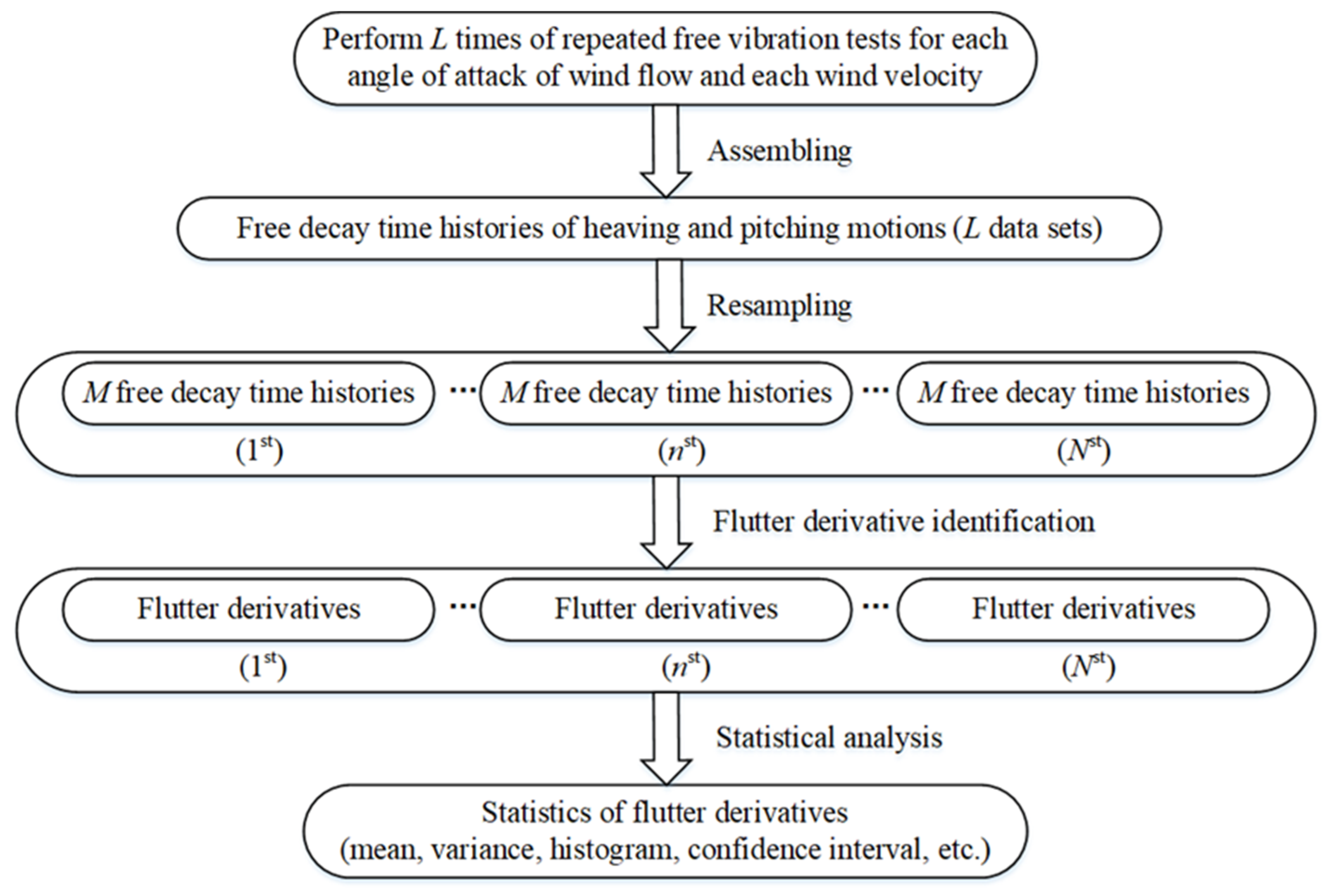
In the system identification process, the bootstrap can be utilized by fully making use of existing information to quantify the uncertainty [31,32,33,34]. In this study, combining with the identification method introduced above, a bootstrap scheme is proposed to quantify the uncertainty of the flutter derivatives. Figure 3 shows the proposed scheme. Firstly, repeated free-vibration tests are performed L times for each angle of attack and wind velocity, and L data sets of free-decay time histories are obtained as the sample population. Secondly, a bootstrap sample of M free-decay time histories is generated by randomly drawing M samples from the sample population. For a practical implementation of this process, firstly number the L data sets, and then generate M random integers that is not smaller than one and not greater than L. Finally take out M samples according to these numbers. N bootstrap samples are obtained by N times of random sampling with replacement. Thirdly, flutter derivative identification is carried out on each bootstrap sample of M free-decay time histories using the proposed optimized weighted least square method with the MABC-Powell algorithm, so that N sets of flutter derivatives are obtained. Lastly, the statistics of the identified flutter derivatives (e.g., mean, standard deviation, and confidence intervals) are calculated by Equations (22)–(24).
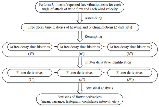
Figure 3.
Bootstrap scheme for statistical identification of flutter derivatives.
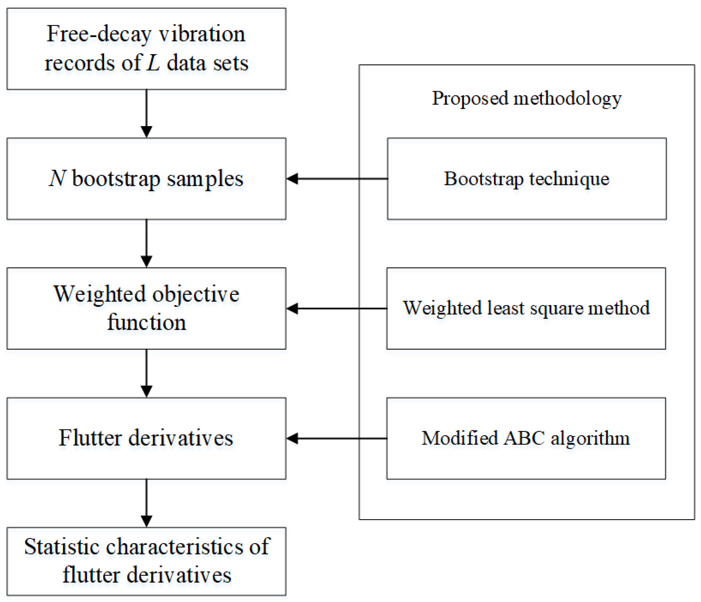
5. The Whole Flow Chart of the Proposed Method
The whole flow chart of the proposed method is shown in Figure 4. Firstly, L free-decay vibration response data sets are obtained by repeated sectional model wind tunnel tests for L times. N bootstrap samples are obtained by bootstrap resampling technique. Then based on the weighted least square principle, the objective function involving each bootstrap sample is established and the optimal weighting factors are obtained by an iterative procedure. When identifying the flutter derivatives by solving the optimization problem, the proposed hybrid method of modified artificial bee colony algorithm and Powell’s algorithm is adopted to improve the accuracy and convergence rate. Finally, based on the set of flutter derivatives identified from each bootstrap sample, the mean and standard deviation of flutter derivatives are calculated, thus not only the optimal value of flutter derivatives, but also their uncertainties are obtained.
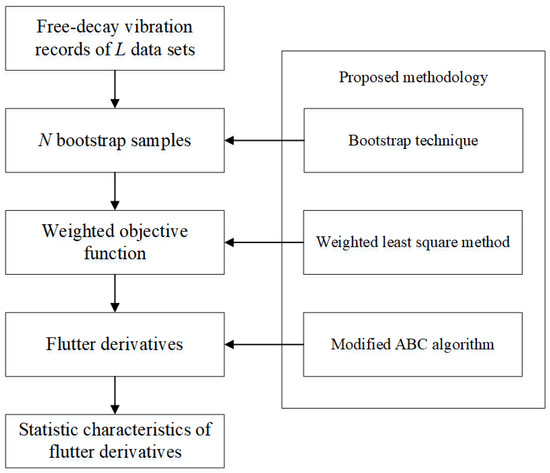
Figure 4.
The whole flowchart of the proposed method.
6. Numerical Illustrative Examples
6.1. Benchmark Functions
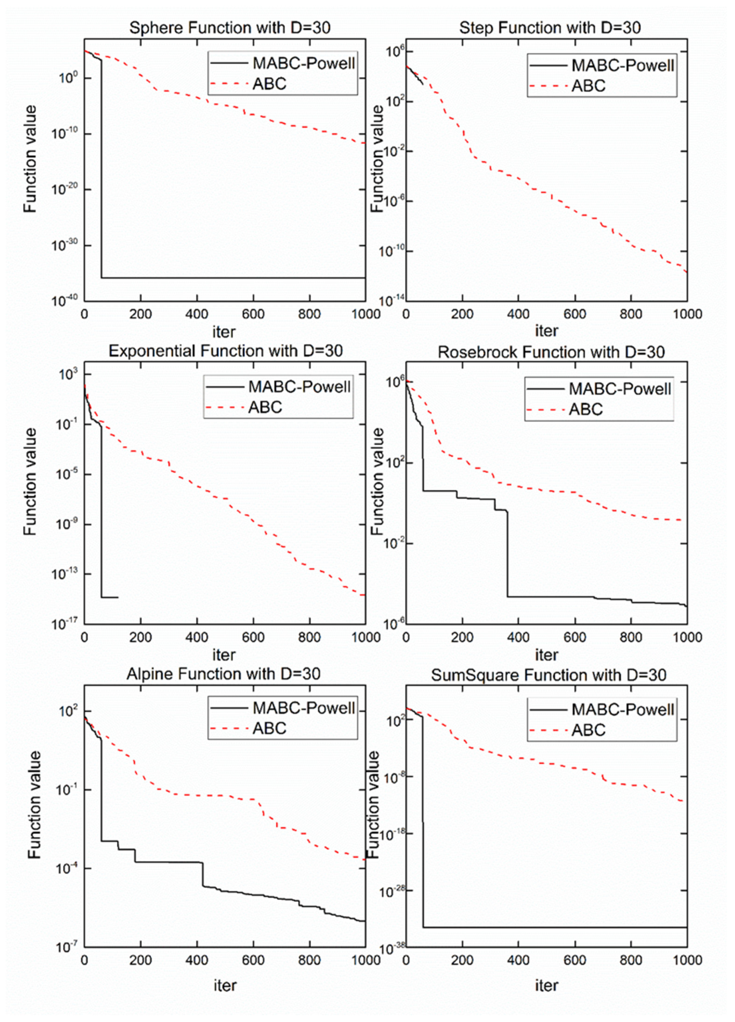
The proposed MABC-Powell method is tested in the optimization solutions of six well-known benchmark functions and compared with the standard ABC algorithm to verify its performance. The details of these benchmark functions are listed in Table 1. In the numerical experiment, the two algorithms are independently run 50 times for each benchmark function. The common parameter settings of the two algorithms are consistent (MCN = 1000, SN = 80, limit = 300). In MABC-Powell, the number of neighbors N is set to 5; the parameters δ and m are set respectively to 150 and 5 in the nonlinear decaying factor; and the number of cycles to launch Powell’s method T is set to 60. The computing hardware of the numerical experiment was a desktop with 3.2 GHz Dual-core Processor and 12 GB RAM, and the software environment was Windows 10 platform.

Table 1.
Test suite with six benchmark functions.
Table 2 shows the experimental results (mean, maximum, and minimum) of the standard ABC and MABC-Powell algorithms for the six benchmark functions with dimension equal to 30. It can be seen that, compared with the standard ABC algorithm, the MABC-Powell algorithm proposed in this paper has better solution accuracy. Figure 5 shows convergence lines for the six benchmark functions obtained with standard ABC and MABC-Powell. It can be seen that, compared with the standard ABC algorithm, the MABC-Powell algorithm has a better convergence rate and solution accuracy. Therefore, MABC-Powell becomes an attractive method for the identification of flutter derivatives. It should be pointed out that since the new algorithm adds an. additional Powell operator, it takes a little more time for the same iteration step. For the Sphere function, 50 times were calculated with MABC-Powell and Standard ABC, respectively, 100 iterations per time, with an average computational time of 1.207 s and 0.215 s per time, respectively. This increase in computation cost is worth it because the computational accuracy is greatly improved.
Table 2.
Accuracy comparison of standard ABC and MABC-Powell on the six benchmark functions with dimension D = 30.
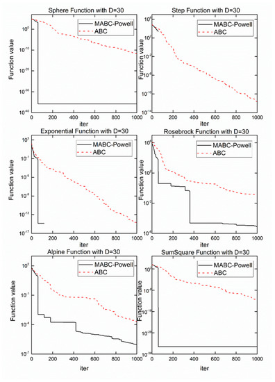
Figure 5.
Convergence lines for the six benchmark functions with dimension equal to 30.
6.2. Numerical Model of a Thin Plate
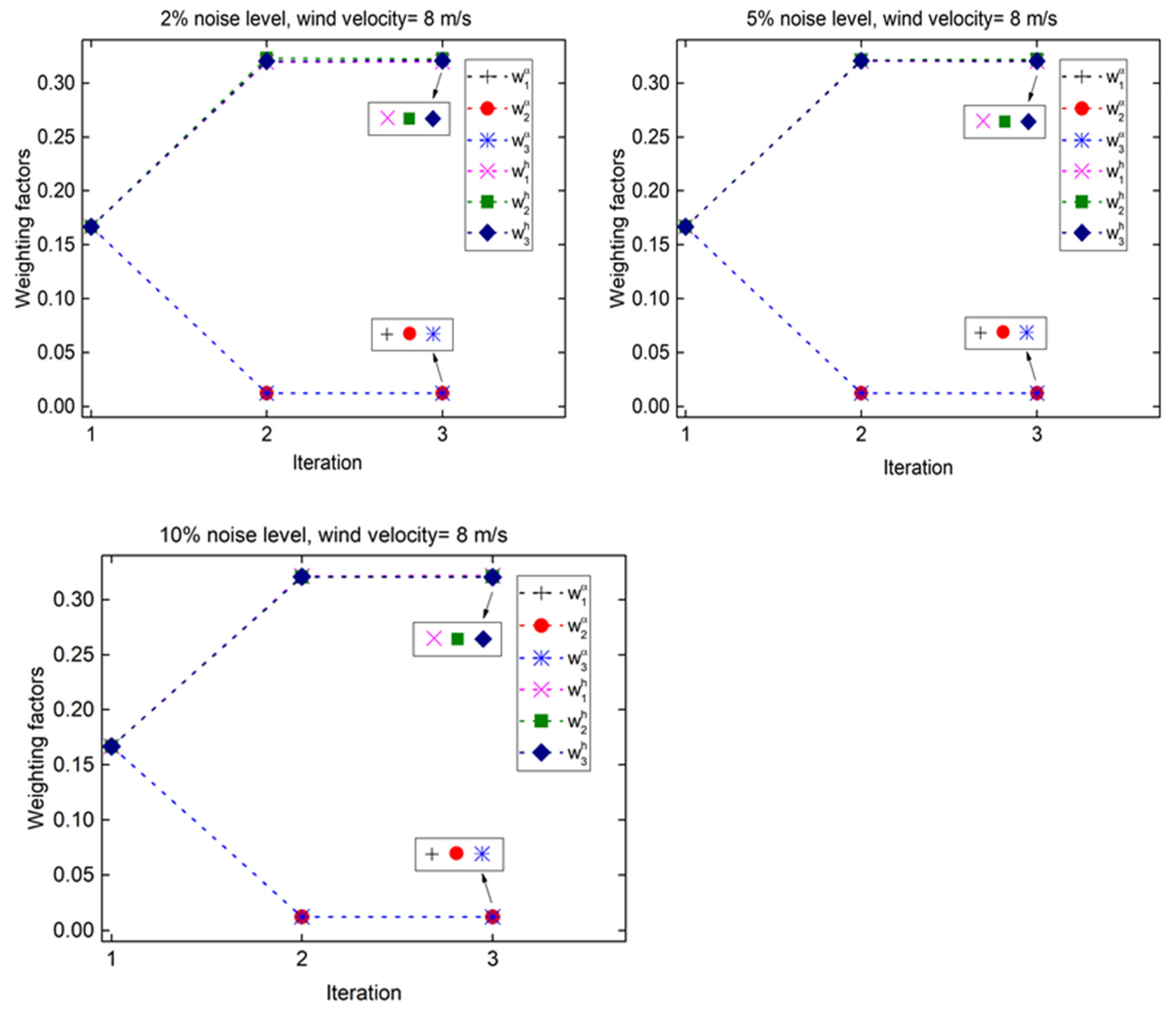
In order to verify the effectiveness and reliability of the proposed method in identifying the flutter derivatives of the bridge deck, the numerical model of a theoretical thin plate section was first employed. The following parameters were used for the numerical model: the width of the thin plate model B was 0.45 m, the mass per unit length m was 11.25 kg/m; the mass moment of inertia per unit length I was 0.2828 kg·m2/m; the frequency of vertical bending mode was 1.9274 Hz; the frequency of torsional mode was 3.0239 Hz; and the damping ratios of vertical bending and torsional modes were both 0.5%. Smooth oncoming wind with 0º angle of attack was assumed. The air density ρ was set to 1.293 kg/m3. In total, 20 sets of free-decay time histories were obtained for each wind speed, and a random noise was superimposed to the simulated response. Three cases of noise level were considered: 2%, 5%, and 10%. These 20 sets of data formed the sample population for bootstrap sampling. The proposed method was used to identify all eight flutter derivatives of the thin plate model. The control parameters in the MABC-Powell for numerical optimization were those specified in the numerical example with benchmark functions. A bootstrap sample consisting of three sets of vertical bending and torsional time histories was randomly selected from the sample population of 20 data sets. Therefore, there were six weighting factors in the objective function: three for vertical bending signal residuals () and the other three for torsional signal residuals (). Figure 6 shows the convergence lines for the six weighting factors for three cases of noise level at a wind velocity of 8 m/s. It is observed that only three iterations are needed for the convergence of weighting factors. In addition, the weighting factors related to torsional signal residuals are generally smaller than those related to vertical bending signal residuals. Please note that the unit of vertical displacement and torsional angle signal is m and rad, respectively. This is probably because the magnitude of torsional signal residuals is larger than that of vertical bending ones. According to Equation (15), the optimal weighting factors are inversely proportional to the related residuals, so the larger the residuals, the smaller the corresponding weighting factors.
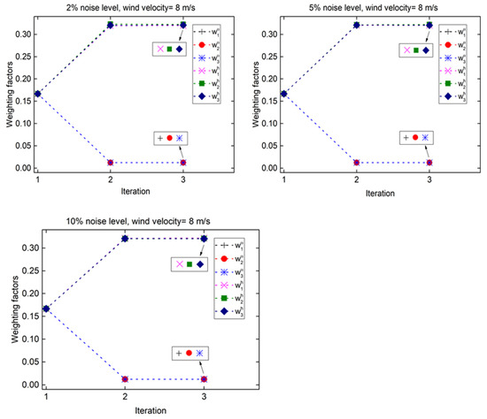
Figure 6.
Convergence lines of weighting factors for thin-plate numerical data.
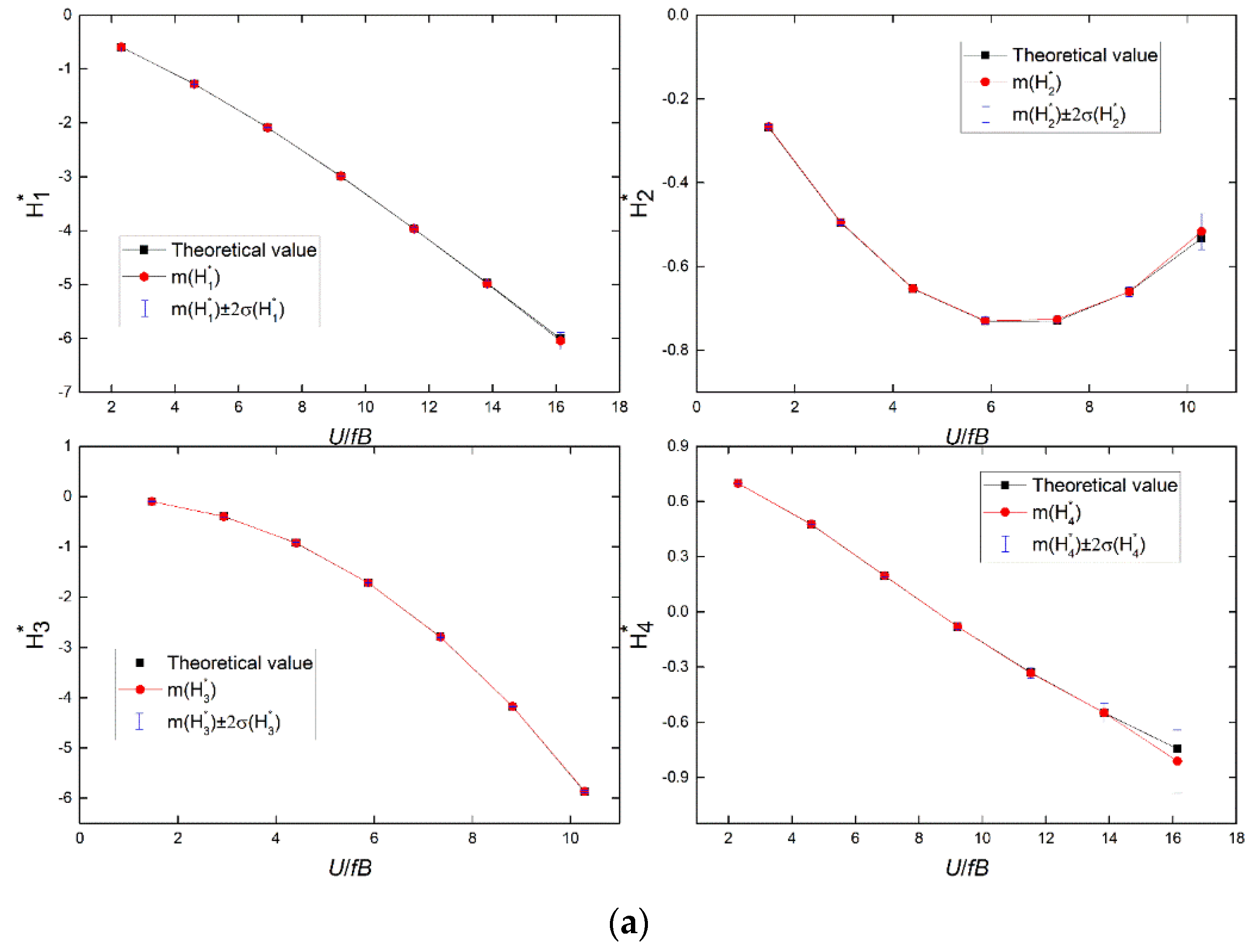
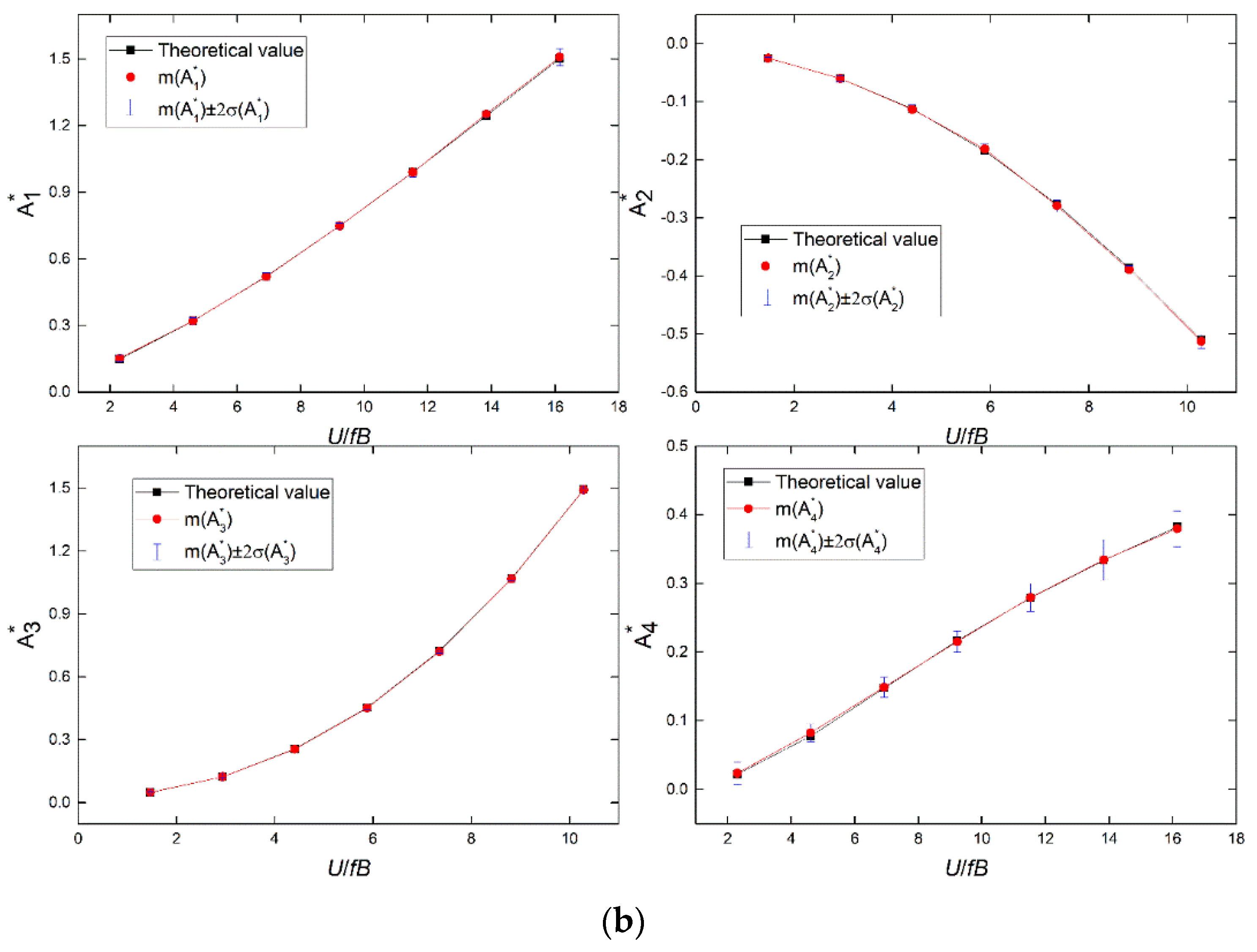
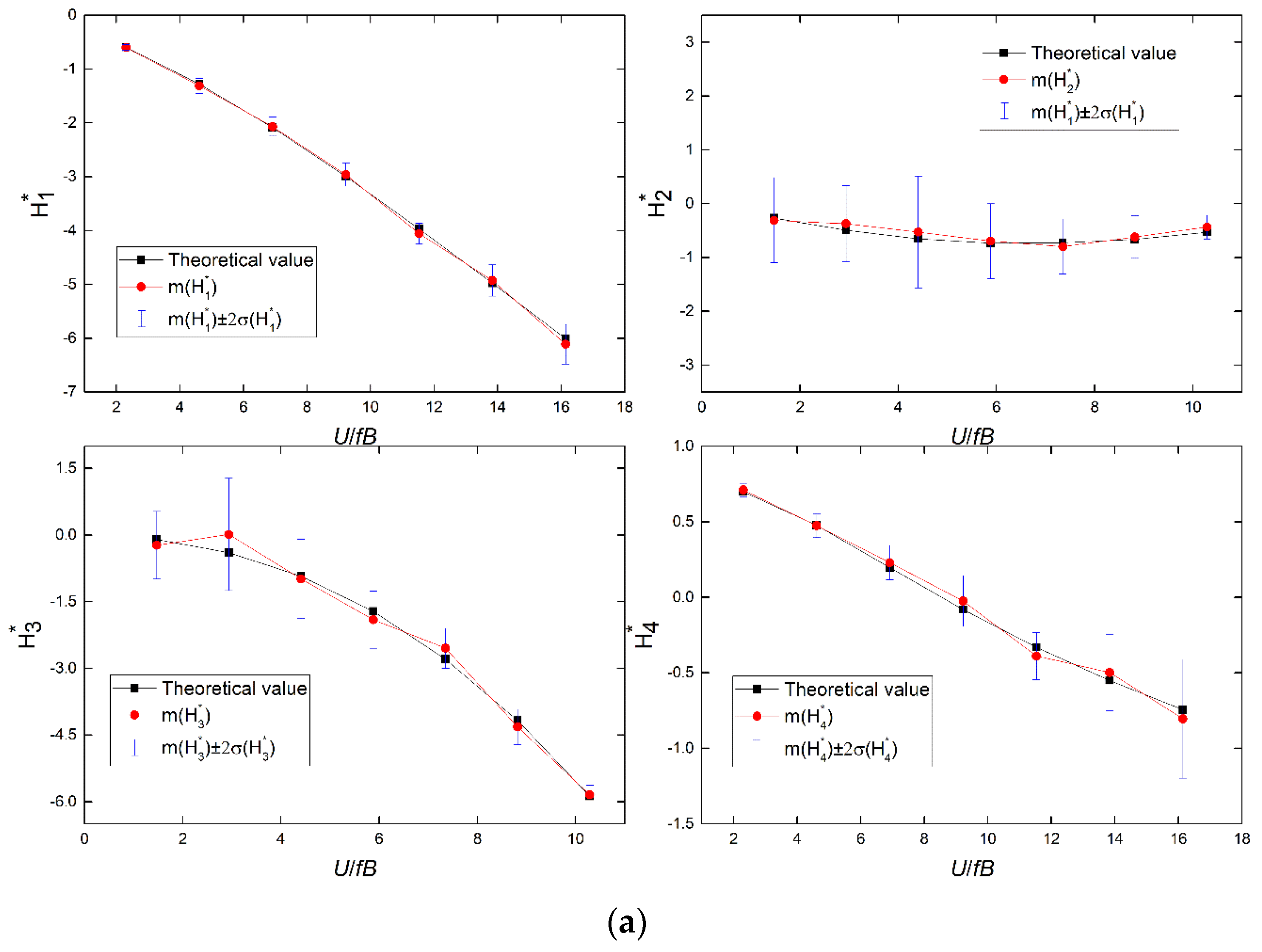
The number of bootstrap samples is 500, i.e., random sampling with replacement was performed 500 times on the population of 20 data sets, and each bootstrap sample consists of three vertical bending and torsional angle time histories. Consequently, the identification process using the proposed method was repeated 500 times, and 500 sets of identified flutter derivatives were obtained. Through statistical analysis of the identified results, mean and standard deviations were obtained. The comparison between flutter derivatives identified by the proposed method and the theoretical values [5] is shown in Figure 6, Figure 7 and Figure 8. The mean and the mean plus or minus two times the standard deviation are shown in the figures. In the case of low noise level (2%, Figure 7), the calculated mean values are nearly perfectly consistent with the theoretical values, and the standard deviations are very small except for , , and at higher wind velocities. In the case of medium noise level (5%, Figure 8), the mean values also agree well with the theoretical counterparts, except for , which shows small deviations from its theoretical value, while relatively large standard deviations are found for , , , , , and at higher wind velocities. Finally, in the case of high noise level (10%, Figure 9), the mean values still agree fairly well with the theoretical values, but the standard deviations are larger than before, especially for , , , and . On the whole, the accuracy of the results is satisfactory, which indicates the effectiveness and reliability of the proposed method for flutter derivative identification.
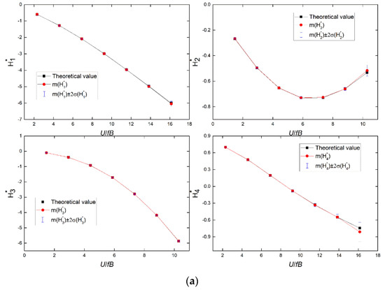
Figure 7.
Comparison of identified flutter derivatives and theoretical solutions for the case of 2% noise level. (a) H*1~ H*4 (2% noise level); (b) A*1~A*4 (2% noise level).
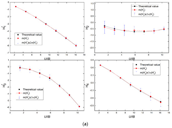
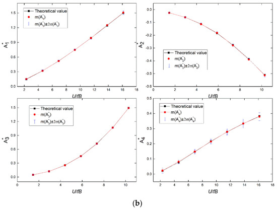
Figure 8.
Comparison of identified flutter derivatives and theoretical solutions for the case of 5% noise level. (a) H*1~H*4 (5% noise level); (b) A*1~A*4 (5% noise level).
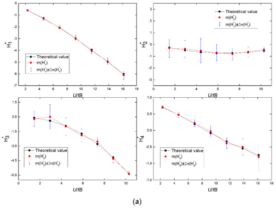
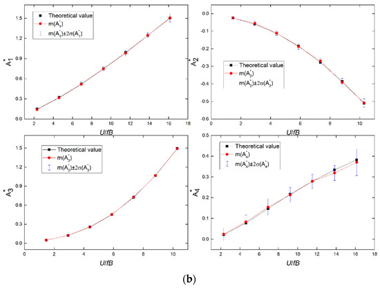
Figure 9.
Comparison of identified flutter derivatives and theoretical solutions for the case of 10% noise level. (a) H*1~H*4 (10% noise level); (b) A*1~A*4 (10% noise level).
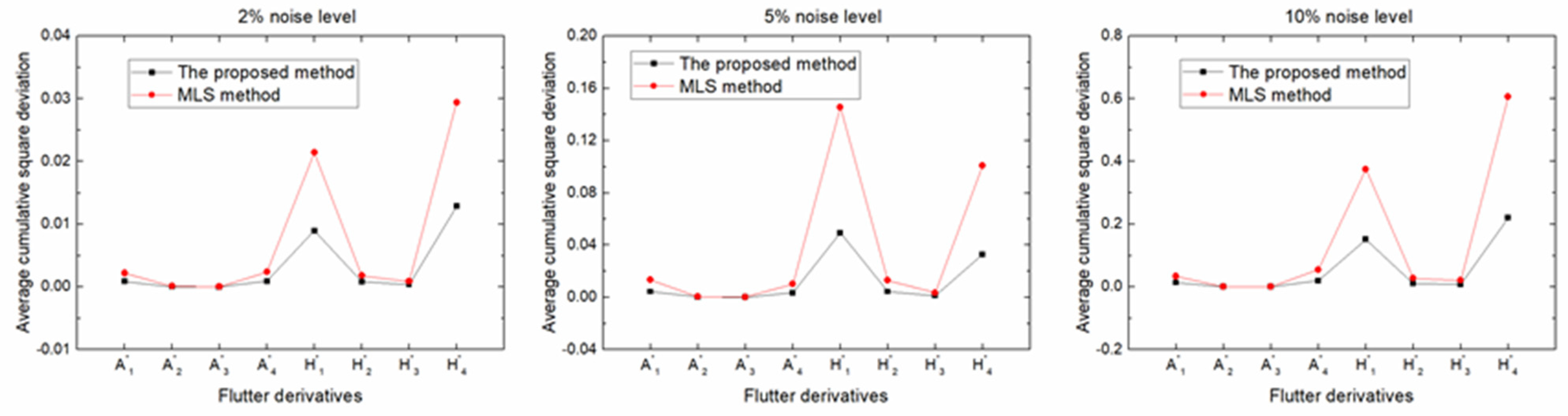
In order to demonstrate the accuracy advantage of this new method in identification of flutter derivatives compared with traditional methods, a comparison study based on the average cumulative square deviations was conducted between the proposed method and MLS method [8]. The average cumulative square deviations were calculated by the following equation:
where is the theoretical value for one of the flutter derivatives, and is the corresponding estimated value calculated on sample j at wind speed i. Ns is the number of samples at each wind speed, and Nw is the number of wind speed. The average cumulative square deviations of identified flutter derivatives and theoretical solutions calculated by the proposed method and MLS method are shown in Figure 10. It is observed that the proposed method has an accuracy advantage in the identification of flutter derivatives compared with MLS under three noise levels. For both methods, although the overall accuracy of H*1 and H*4 is worse than that of other flutter derivatives, the proposed method is better than MLS with respect to these two flutter derivatives.
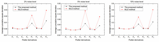
Figure 10.
Average cumulative square deviations of identified flutter derivatives and theoretical solutions calculated by the proposed method and MLS method.
The mean, standard deviation (σ), coefficient of variation (CV), and 95%-confidence interval (CI) of flutter derivatives for three noise levels at a wind velocity of 8 m/s, together with their theoretical values are reported in Table 3, Table 4 and Table 5. From the tables, it is observed that the means agree with the theoretical values as a whole, while the standard deviations increase with the noise level. It is also worth noting that the theoretical values are all within the 95%-confidence intervals.
Table 3.
Bootstrap statistics of identified flutter derivatives with 2% noise level (U = 8 m/s).
Table 4.
Bootstrap statistics of identified flutter derivatives with 5% noise level (U = 8 m/s).
Table 5.
Bootstrap statistics of identified flutter derivatives with 10% noise level (U = 8 m/s).
7. Example with Sectional Model of Bridge Deck in Wind Tunnel Tests
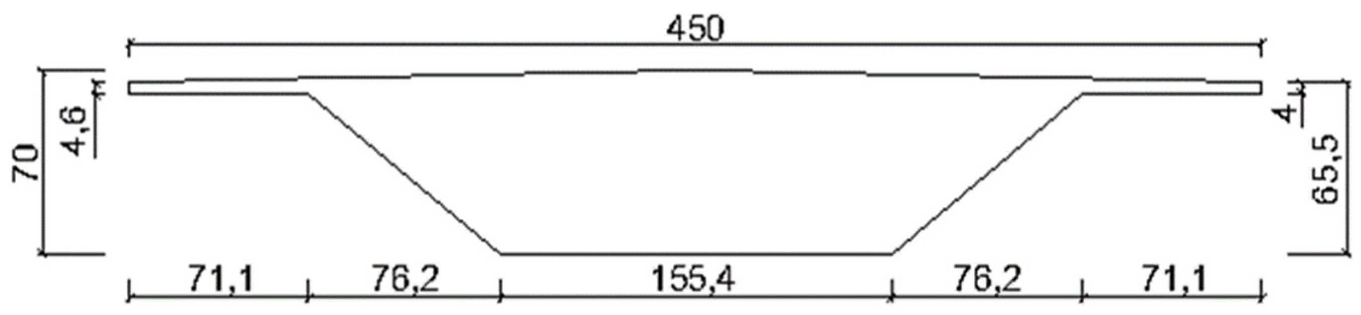
In order to further investigate the reliability of the proposed method for flutter derivative identification through wind tunnel tests, experimental data for a sectional model of a bridge deck were used. Free-vibration wind tunnel tests were carried out in the CRIACIV laboratory. Figure 11 shows the cross-section view of the model. It has a width B of 450 mm and a depth H of 70 mm. The model was suspended elastically by eight helical springs, allowing for vertical and torsional motions, while suppressing the sway motion in the wind flow direction by long cables. Vertical and torsional initial conditions were set through a device consisting of cables and electromagnets. More details concerning the model, the setup, and the wind tunnel test can be found in [19,35]. The free vibration tests were repeated 10 times for each wind speed.
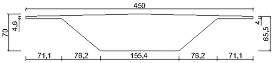
Figure 11.
Cross-section geometry of the model tested in the wind tunnel (in mm).
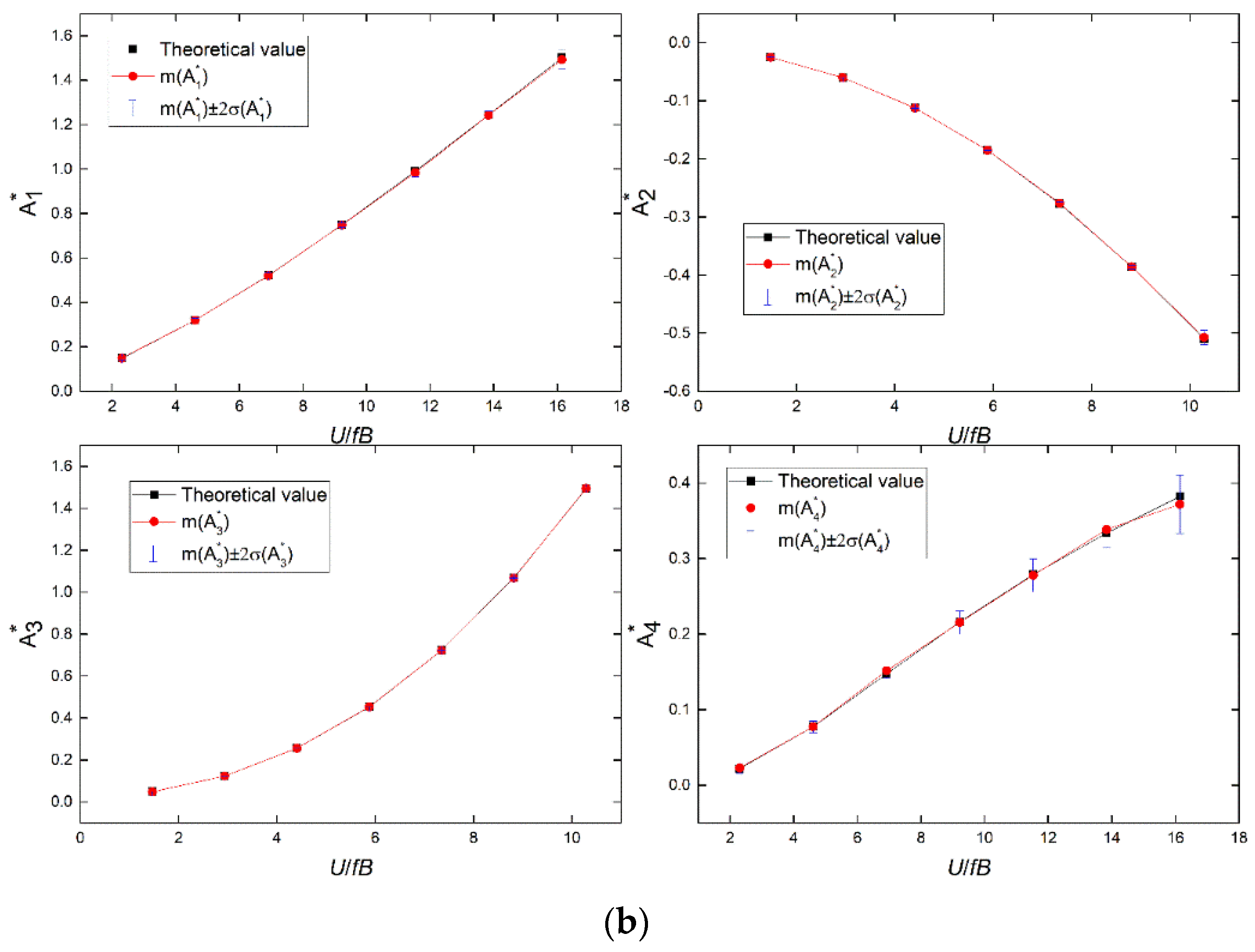
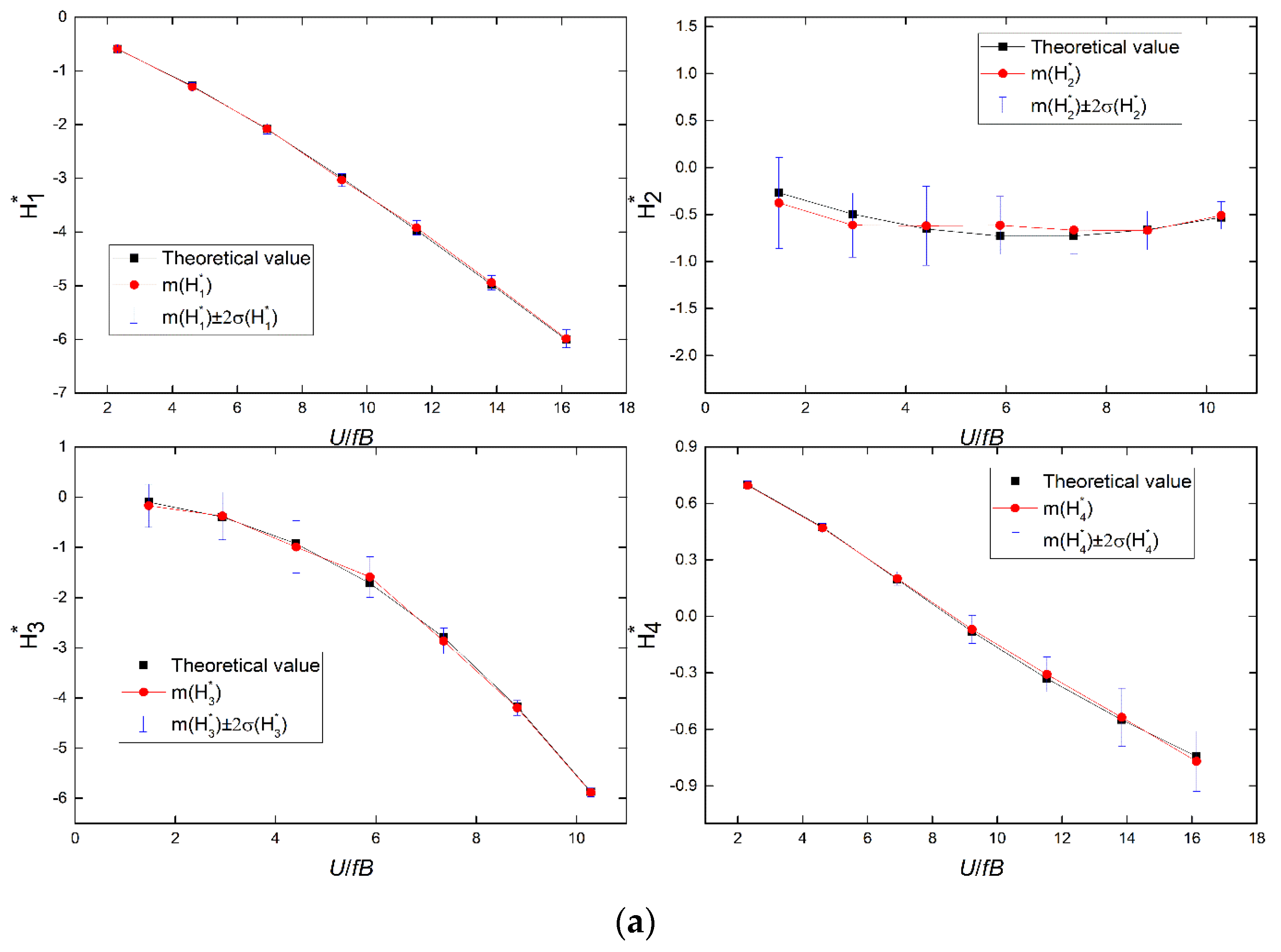
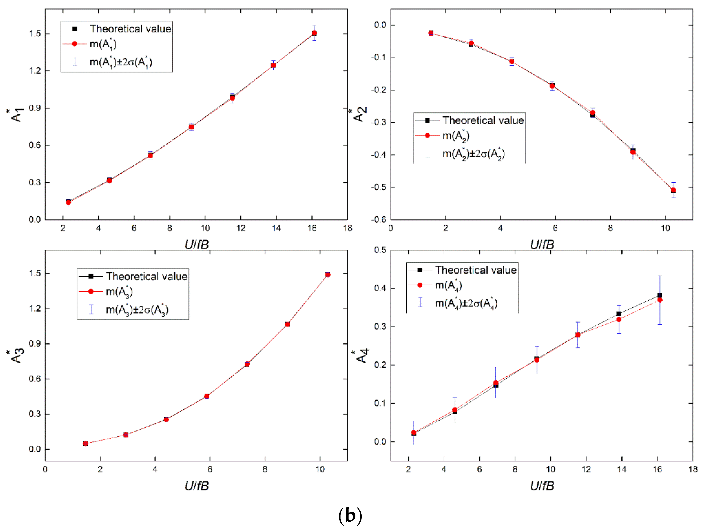
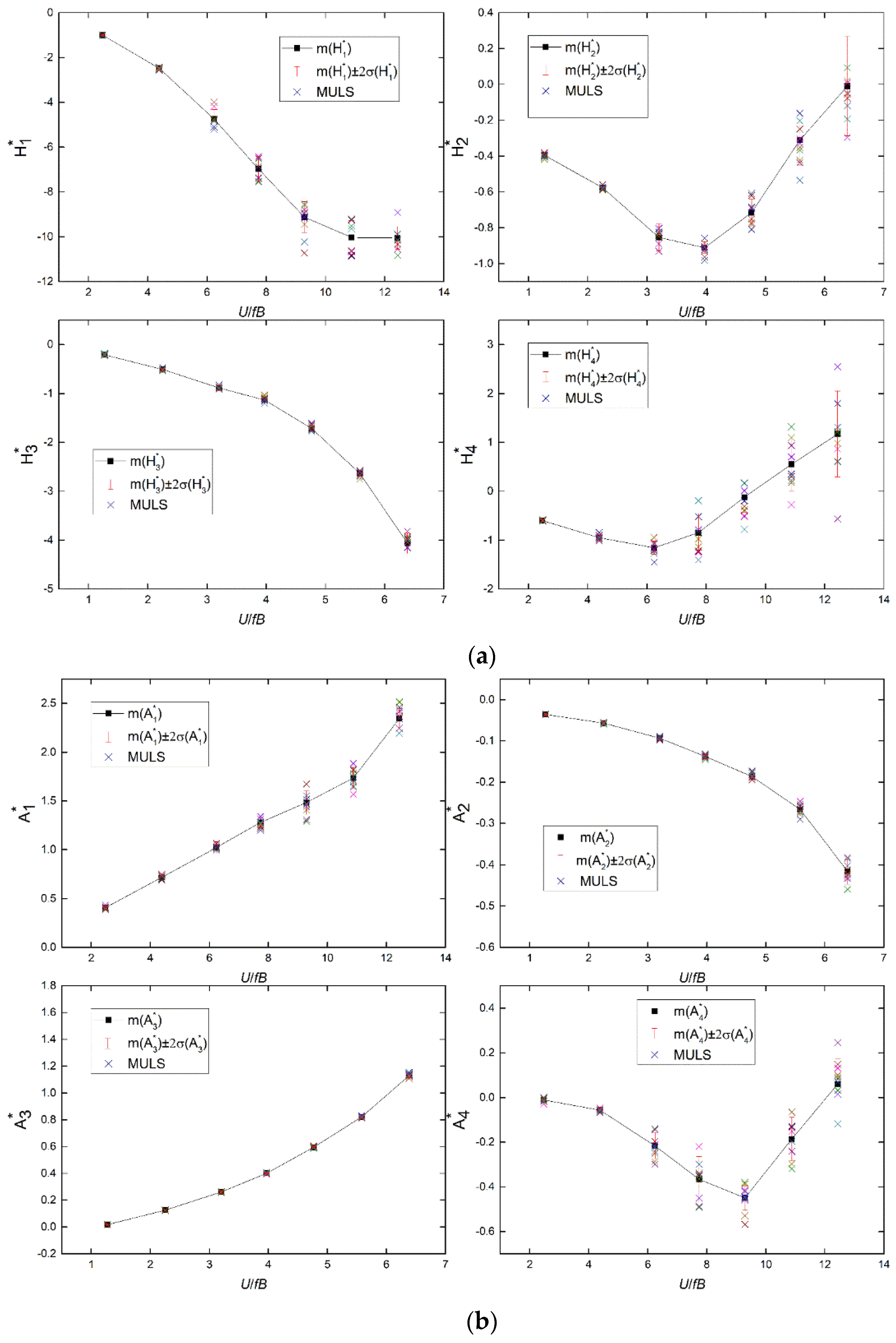
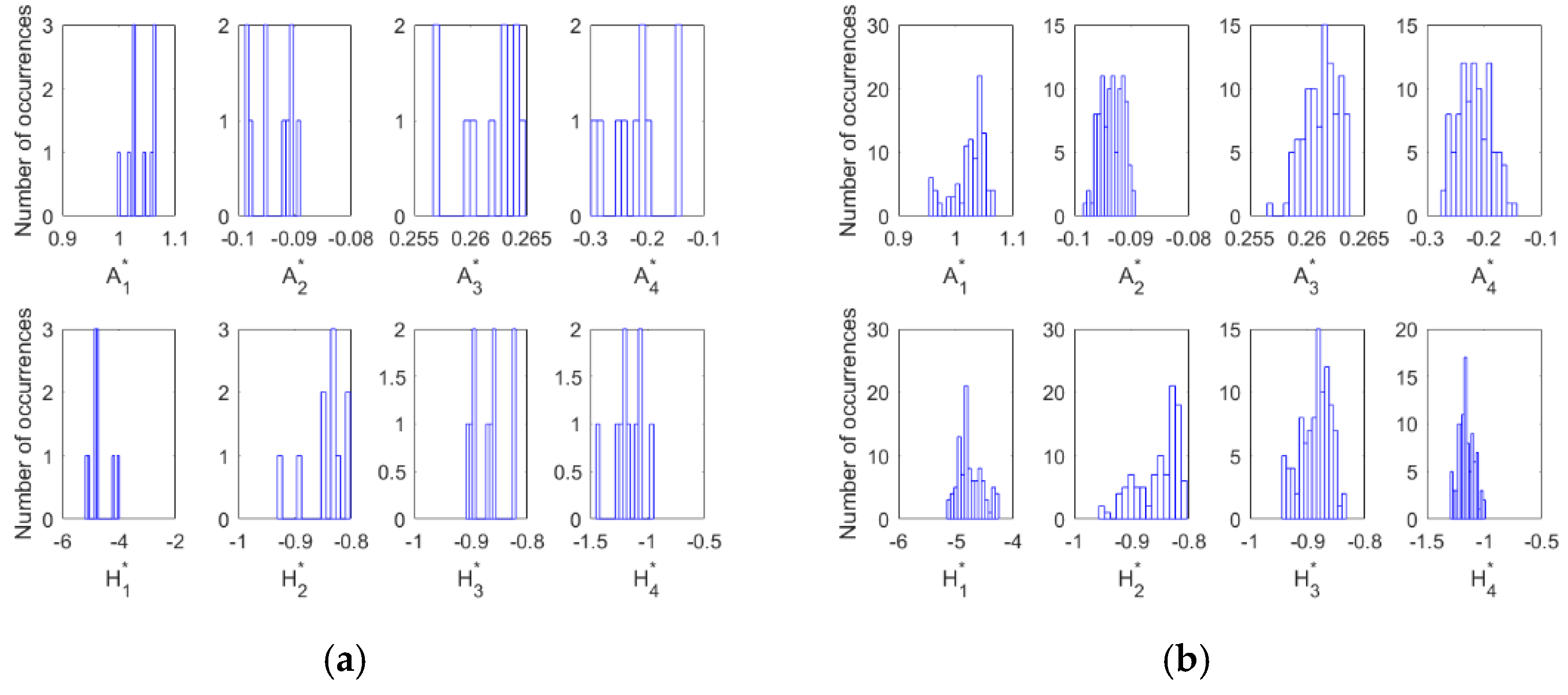
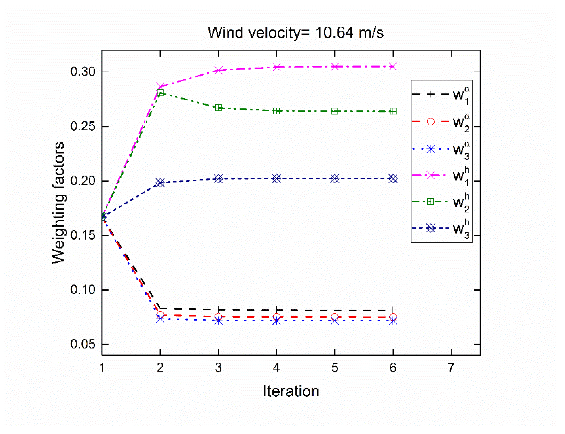
The sample population for bootstrap sampling consisted of 10 sets of data. All eight flutter derivatives of the bridge deck model were identified by the proposed method, in which the control parameters in the MABC-Powell algorithm for numerical optimization are the same as in the numerical examples in the previous sections. The number of data sets in each bootstrap sample is still three. In total, 100 bootstrap samples are extracted from the sample population of 10 data sets. The comparison between the flutter derivatives identified by the proposed method and the reference results [19] is shown in Figure 12. At a certain testing wind speed, the real frequencies were used for the calculation of reduced wind velocities U/fB. It can be seen that the flutter derivatives identified by the proposed method agree with the reference results and exhibit consistent statistical properties. , , and have small standard deviations while the other derivatives are more dispersed. The standard deviations at higher wind speed are generally larger than those at lower wind speed, especially near flutter onset. The possible reasons for this phenomenon are presented in point (3) of the discussion part. It should also be noted that the reference results present only 10 samples, which is insufficient to obtain accurate statistics. To improve statistical inference, the bootstrap scheme with 100 samples is adopted. At the wind speed of 8.6 m/s, the histogram of flutter derivatives identified using only the original 10 data sets and the histogram of flutter derivatives identified using 100 bootstrap samples are shown in Figure 13a,b, respectively. It can be seen that the distribution in Figure 13b is more concentrated, while Figure 13a is very scattered. The convergence lines for the weighting factors for one bootstrap sample at a wind speed of 10.64 m/s are shown in Figure 14. Additionally, in this case, the weighting factors for torsional signal residuals are smaller than those for the vertical bending ones, which are similar to the results of the numerical example. Please note that the unit of torsional and vertical bending signal is m and rad, respectively. This phenomenon is also similar to the proposed weighting factors in [10].
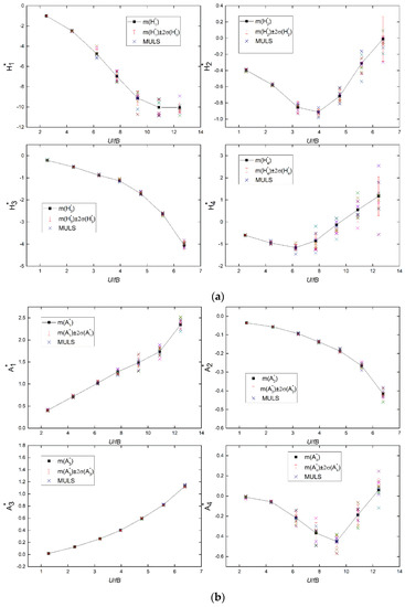
Figure 12.
Results of the flutter derivatives identified with the proposed method from experimental wind tunnel data and comparison with the values in [19] obtained with the MULS method. (a) H*1~H*4 for experimental data; (b) A*1~A*4 for experimental data.
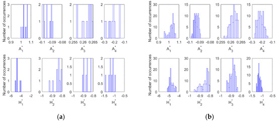
Figure 13.
Histogram comparison of flutter derivatives identified from 100 bootstrap samples and 10 original data sets (U = 8.6 m/s). (a) 10 original data sets; (b) 100 bootstrap samples.
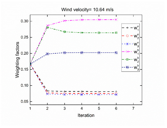
Figure 14.
Convergence lines of weighting factors for experimental data.
8. Discussions
The main purpose and contribution of this study was to propose three improvement measures based on the traditional linear Scanlan’s flutter model and the least square principle, thus providing a new way of thinking for flutter derivative identification. Firstly, a new method of determining weighting factors in the least square objective function is proposed. Secondly, the original ABC algorithm is improved and applied to flutter derivative identification. Thirdly, the uncertainty of flutter derivatives is quantified by the bootstrap method. Since the model in this paper is based on traditional assumptions and needs further improvement in some aspects, the relevant problems are listed below for further discussion and improvement in future studies.
- The first issue is the aeroelastic coupling effect of vertical and torsional modes at non-zero wind speed. For a 2-DOF sectional model system, there are always two natural modes (vertical and torsional) at any wind speed, and their frequencies and mode shapes vary with wind speed. Thus, each of the vertical and torsional motion in the free-decay vibration tests at non-zero wind speed contains components of both frequencies, and therefore, there are two sets of eight frequency-dependent flutter derivatives (i.e., 16 unknown parameters) to be identified. However, these two sets of eight flutter derivatives cannot be uniquely identified if only the free vibration response of a 2-DOF bridge sectional model at one wind speed is given. An approximation is always made in most traditional identification methods as well as our method (Equations (5) and (6)) that the flutter derivatives related to the vertical motion are dominated by the first frequency component and contrarily those related to the torsional motion are dominated by the second frequency component. This approximation may lead to error or scattering of identified flutter derivatives. This implied approximation in the identification of flutter derivatives has been deeply discussed by Chen and Kareem [36]. Their parametric study shows that excellent agreement was obtained despite the approximation in the self-excited forces being made, which supports the efficacy of this approximation.
- The second issue is the nonlinear vibration characteristics of the bridge deck sectional model. The identification of flutter derivatives involves a step of extraction of the stiffness and damping coefficients in still air, which include both mechanical and aerodynamic components. In most traditional identification methods as well as our method, the mechanical components in still air are conventionally assumed constants, while the aerodynamic components in still air are neglected. These assumptions will inevitably lead to some error of the identified flutter derivatives. Actually, the mechanical damping ratios and natural frequencies of the spring-suspended sectional model system vary to some extent with the change of the oscillating amplitude [37], and the aerodynamic damping ratio and frequency in still air vary with the vibration amplitude as well [38,39]. It was found that the aerodynamic components were more sensitive to the vibration amplitude than the mechanical components.
- Treatment of the data at high wind speed especially near flutter onset is a challenging and difficult issue in flutter derivative identification. In the higher wind speed cases, especially in the cases of wind speeds close to the critical point of flutter, the second frequency component is absolutely dominant in both the vertical and torsional responses, and the first frequency component almost vanishes. The reason is that the aerodynamic damping for the first mode is always positive for the flat bridge decks and rapidly increases with the rise of the wind speed while the aerodynamic damping for the second mode decreases in general and even becomes negative. Thus, the approximation made in point (1) will lead to large errors. Another critical point may be the high aerodynamic nonlinearity near flutter onset. The Scanlan’s linear model of self-excited forces may be improper for modeling the aerodynamic characteristics near flutter onset. The modeling errors cause significant scattering of identified flutter derivatives near the flutter critical wind speed.
9. Conclusions
A new algorithm to extract eight flutter derivatives and also quantify their uncertainties simultaneously from free-vibration records in wind-tunnel tests is presented. It is based on the least squares principle, but it introduces three basic modifications to enhance the identification. The first contribution of this paper is the introduction of rational weighting factors in the error function, which are optimized by an iterative procedure. The second contribution is the use of the heuristic MABC-Powell algorithm to solve the optimization problem and achieve better convergence and accuracy. The third original aspect is the adoption of a bootstrap scheme for uncertainty quantification and statistical inference of the identified flutter derivatives when only few data samples are available. The proposed MABC-Powell algorithm for numerical optimization was tested on several benchmark functions, showing better performance compared to standard ABC in terms of both the convergence rate and accuracy. The flutter derivatives identification method was verified through both a numerical and an experimental example. In both cases, the identified results showed good agreement with theoretical solutions or reference values, which indicates the effectiveness and robustness of the proposed method.
Author Contributions
Conceptualization, Z.F.; Investigation, Z.F. and Y.L.; Methodology, Z.F.; Software, Y.L.; Writing—original draft, Z.F. and Y.L.; Writing—review & editing, Z.F. All authors have read and agreed to the published version of the manuscript.
Funding
This work has partially been supported by National Natural Science Foundation of China (Grant No. 52178284, 51708203), the Open Research Fund Program for innovation platforms of universities in Hunan province from the Education Department of Hunan Province (Grant No. 17K022), and the Fundamental Research Funds for the Central Universities (Grant No. 531118010047). These supports are gratefully acknowledged.
Institutional Review Board Statement
Not applicable.
Informed Consent Statement
Not applicable.
Data Availability Statement
Data supporting reported results can be provided if requested.
Acknowledgments
The authors would like to thank Claudio Mannini at University of Florence for providing the experimental data and constructive comments on the paper manuscript.
Conflicts of Interest
The authors declare no conflict of interest.
Appendix A
The pseudo-code of the standard ABC algorithm is given below:
| Algorithm A1 Standard ABC algorithm |
| Input |
| D: Dimension of x |
| f(x): Objective function, x = |
| xmax: Upper bound of x |
| xmin: Lower bound of x |
| Output |
| : Optimal solution |
| /*Parameters initialization*/ |
| MCN: Max cycle number |
| SN: Half of population size |
| limit: Number of cycles for abandonment |
| iter: Iterations of the algorithm |
| /*Population initialization*/ |
| for i = 1 to SN do |
| for j = 1 to D do |
| end for |
| trial(i) = 0 |
| end for |
| while (iter < MCN) do |
| /*The employed bee phase*/ |
| for i = 1 to SN do |
| Randomly choose j from {1, 2, …, D} and k from {1, 2, …, SN} that k ≠ i |
| Randomly choose from [−1,1] |
| if trial(i) = 0 |
| else trial(i) = trial(i)+1 |
| end if |
| end for |
| = best() |
| /*The onlookers phase*/ |
| fori = 1 to SN do |
| end for |
| fori = 1 to SN do |
| q = roultteWheel |
| Randomly choose from [−1,1] |
| Randomly choose j from {1, 2, …, D} and k from {1, 2, …, SN} that k ≠ i |
| if trial(i) = 0 |
| else trial(q) = trial(q)+1 |
| end if |
| end for |
| = best() |
| /*The scouts phase*/ |
| for i = 1 to SN do |
| if trial(i) > limit |
| for j = 1 to D do |
| end for |
| end if |
| end for |
| iter = iter + 1 |
| end while (m = MCN) |
Appendix B
The pseudo-code of the Modified ABC algorithm with Powell’s method is given below:
| Algorithm A2 Modified ABC algorithm with Powell’s method (MABC-Powell) |
| Input |
| D: Dimension of x |
| f(x): Objective function, x = |
| xmax: Upper bound of x |
| xmin: Lower bound of x |
| Output |
| : Optimal solution |
| /*Parameters initialization*/ |
| MCN: Max cycle number |
| SN: Half of population size |
| limit: Number of cycles for abandonment |
| iter: Iterations of the algorithm |
| /*Population initialization*/ |
| for i = 1 to SN do |
| for j = 1 to D do |
| end for |
| trial(i) = 0 |
| end for |
| while (iter < MCN) do |
| /*The employed bee phase*/ |
| for i = 1 to SN do |
| Randomly choose j from {1, 2, …, D} |
| Randomly choose from [−1,1] |
| Randomly choose N neighbors and calculate the best neighbor |
| if trial(i) = 0 |
| else trial(i) = trial(i)+1 |
| end if |
| end for |
| = best() |
| /*The onlookers phase*/ |
| fori = 1 to SN do |
| end for |
| fori = 1 to SN do |
| q = roultteWheel |
| Randomly choose from [−1,1] |
| Randomly choose j from {1, 2, …, D} |
| Randomly choose N neighbors and calculate the best neighbor |
| if trial(i) = 0 |
| else trial(q) = trial(q)+1 |
| end if |
| end for |
| = best() |
| /*The Powell’s method phase*/ |
| if mod(iter,T) = 0 do |
| Randomly choose k from {1, 2, …, D} that has to be different from best, |
| generate a new solution U |
| Use the U as a starting point and generate a new solution by Powell’s method |
| if trial(i) = 0 |
| else trial(k) = trial(k)+1 |
| end if |
| end if |
| /*The scouts phase*/ |
| for i = 1 to SN do |
| if trial(i) > limit |
| for j = 1 to D do |
| end for |
| end if |
| end for |
| iter = iter + 1 |
| end while (iter = MCN) |
References
- Lin, P.; Hu, G.; Li, C.; Li, L.; Xiao, Y.; Tse, K.T.; Kwok, K.C.S. Machine learning-based prediction of crosswind vibrations of rectangular cylinders. J. Wind Eng. Ind. Aerodyn. 2021, 211, 104549. [Google Scholar] [CrossRef]
- Hu, G.; Kwok, K.C.S. Predicting wind pressures around circular cylinders using machine learning techniques. J. Wind Eng. Ind. Aerodyn. 2020, 198, 104099. [Google Scholar] [CrossRef]
- Hu, G.; Liu, L.; Tao, D.; Song, J.; Tse, K.T.; Kwok, K.C.S. Deep learning-based investigation of wind pressures on tall building under interference effects. J. Wind Eng. Ind. Aerodyn. 2020, 201, 104138. [Google Scholar] [CrossRef]
- Diana, G.; Rocchi, D.; Belloli, M. Wind tunnel: A fundamental tool for long-span bridge design. Struct. Infrastruct. Eng. 2015, 11, 533–555. [Google Scholar] [CrossRef]
- Scanlan, R.H.; Tomko, J.J. Airfoil and bridge deck flutter derivatives. J. Eng. Mech. Div. 1971, 97, 1717–1737. [Google Scholar] [CrossRef]
- Sarkar, P.P.; Jones, N.P.; Scanlan, R.H. System identification for estimation of flutter derivatives. J. Wind Eng. Ind. Aerodyn. 1992, 42, 1243–1254. [Google Scholar] [CrossRef]
- Gu, M.; Zhang, R.; Xiang, H. Identification of flutter derivatives of bridge decks. J. Wind Eng. Ind. Aerodyn. 2000, 84, 151–162. [Google Scholar] [CrossRef]
- Ding, Q.S.; Chen, A.R.; Xiang, H.F. Modified least-square method for identification of bridge deck aerodynamic derivatives. J. Tongji Univ. 2001, 29, 25–29. [Google Scholar]
- Li, Y.; Liao, H.; Qiang, S. Weighting ensemble least-square method for flutter derivatives of bridge decks. J. Wind Eng. Ind. Aerodyn. 2003, 91, 713–721. [Google Scholar] [CrossRef]
- Bartoli, G.; Contri, S.; Mannini, C.; Righi, M. Toward an Improvement in the Identification of Bridge Deck Flutter Derivatives. J. Eng. Mech. 2009, 135, 771–785. [Google Scholar] [CrossRef]
- Xu, F.Y.; Chen, X.Z.; Cai, C.S.; Chen, A.R. Determination of 18 Flutter Derivatives of Bridge Decks by an Improved Stochastic Search Algorithm. J. Bridg. Eng. 2012, 17, 576–588. [Google Scholar] [CrossRef]
- BogunovićJakobsen, J.; Hjorth-Hansen, E. Determination of the aerodynamic derivatives by a system identification method. J. Wind Eng. Ind. Aerodyn. 1995, 57, 295–305. [Google Scholar] [CrossRef]
- Brownjohn, J.M.W.; Jakobsen, J.B. Strategies for aeroelastic parameter identification from bridge deck free vibration data. J. Wind Eng. Ind. Aerodyn. 2001, 89, 1113–1136. [Google Scholar] [CrossRef]
- Karaboga, D. An Idea Based on Honey Bee Swarm for Numerical Optimization; Erciyes University: Kayseri, Turkey, 2005. [Google Scholar]
- Sun, H.; Luş, H.; Betti, R. Identification of structural models using a modified Artificial Bee Colony algorithm. Comput. Struct. 2013, 116, 59–74. [Google Scholar] [CrossRef]
- Gao, W.; Liu, S.; Huang, L. A novel artificial bee colony algorithm with Powell’s method. Appl. Soft Comput. 2013, 13, 3763–3775. [Google Scholar] [CrossRef]
- Sun, H.; Betti, R. A Hybrid Optimization Algorithm with Bayesian Inference for Probabilistic Model Updating. Comput. Civ. Infrastruct. Eng. 2015, 30, 602–619. [Google Scholar] [CrossRef]
- Peng, H.; Deng, C.; Wu, Z. Best neighbor-guided artificial bee colony algorithm for continuous optimization problems. Soft Comput. 2019, 23, 8723–8740. [Google Scholar] [CrossRef]
- Mannini, C.; Bartoli, G. Aerodynamic uncertainty propagation in bridge flutter analysis. Struct. Saf. 2015, 52, 29–39. [Google Scholar] [CrossRef]
- Pourzeynali, S.; Datta, T.K. Reliability analysis of suspension bridges against flutter. J. Sound Vib. 2002, 254, 143–162. [Google Scholar] [CrossRef] [Green Version]
- Cheng, J.; Cai, C.S.; Xiao, R.; Chen, S.R. Flutter reliability analysis of suspension bridges. J. Wind Eng. Ind. Aerodyn. 2005, 93, 757–775. [Google Scholar] [CrossRef]
- Baldomir, A.; Kusano, I.; Hernandez, S.; Jurado, J.A. A reliability study for the Messina Bridge with respect to flutter phenomena considering uncertainties in experimental and numerical data. Comput. Struct. 2013, 128, 91–100. [Google Scholar] [CrossRef]
- Abbas, T.; Morgenthal, G. Framework for sensitivity and uncertainty quantification in the flutter assessment of bridges. Probabilistic Eng. Mech. 2016, 43, 91–105. [Google Scholar] [CrossRef]
- Stanford, B.; Beran, P. Computational strategies for reliability-based structural optimization of aeroelastic limit cycle oscillations. Struct. Multidiscip. Optim. 2012, 45, 83–99. [Google Scholar] [CrossRef]
- Kusano, I.; Baldomir, A.; Jurado, J.A.; Hernández, S. Reliability based design optimization of long-span bridges considering flutter. J. Wind Eng. Ind. Aerodyn. 2014, 135, 149–162. [Google Scholar] [CrossRef]
- Kusano, I.; Baldomir, A.; Jurado, J.Á.; Hernández, S. The importance of correlation among flutter derivatives for the reliability based optimum design of suspension bridges. Eng. Struct. 2018, 173, 416–428. [Google Scholar] [CrossRef]
- Efron, B.; Tibshirani, R. An Introduction to the Bootstrap; Chapman & Hall: New York, NY, USA, 1993; Volume 57, ISBN 0412042312. [Google Scholar]
- Christodoulou, K.; Papadimitriou, C. Structural identification based on optimally weighted modal residuals. Mech. Syst. Signal Process. 2007, 21, 4–23. [Google Scholar] [CrossRef]
- Zhu, G.; Kwong, S. Gbest-guided artificial bee colony algorithm for numerical function optimization. Appl. Math. Comput. 2010, 217, 3166–3173. [Google Scholar] [CrossRef]
- Powell, M.J.D. Restart procedures for the conjugate gradient method. Math. Program. 1977, 12, 241–254. [Google Scholar] [CrossRef]
- Bittanti, S.; Lovera, M. Bootstrap-based estimates of uncertainty in subspace identification methods. Automatica 2000, 36, 1605–1615. [Google Scholar] [CrossRef]
- Kijewski, T.; Kareem, A. On the reliability of a class of system identification techniques: Insights from bootstrap theory. Struct. Saf. 2002, 24, 261–280. [Google Scholar] [CrossRef]
- Yan, B.F.; Miyamoto, A.; Brühwiler, E. Wavelet transform-based modal parameter identification considering uncertainty. J. Sound Vib. 2006, 291, 285–301. [Google Scholar] [CrossRef]
- Feng, Z.Q.; Zhao, B.; Hua, X.G.; Chen, Z.Q. Enhanced EMD-RDT Method for Output-Only Ambient Modal Identification of Structures. J. Aerosp. Eng. 2019, 32, 04019046. [Google Scholar] [CrossRef]
- Mannini, C.; Šoda, A.; Voß, R.; Schewe, G. Unsteady RANS simulations of flow around a bridge section. J. Wind Eng. Ind. Aerodyn. 2010, 98, 742–753. [Google Scholar] [CrossRef] [Green Version]
- Chen, X.; Kareem, A. Efficacy of the implied approximation in the identification of flutter derivatives. J. Struct. Eng. 2004, 130, 2070–2074. [Google Scholar] [CrossRef]
- Gao, G.; Zhu, L. Nonlinearity of mechanical damping and stiffness of a spring-suspended sectional model system for wind tunnel tests. J. Sound Vib. 2015, 355, 369–391. [Google Scholar] [CrossRef]
- Cao, F.; Ge, Y. Air-induced nonlinear damping and added mass of vertically vibrating bridge deck section models under zero wind speed. J. Wind Eng. Ind. Aerodyn. 2017, 169, 217–231. [Google Scholar] [CrossRef]
- Zhang, M.; Xu, F. Nonlinear Vibration Characteristics of Bridge Deck Section Models in Still Air. J. Bridg. Eng. 2018, 23, 04018059. [Google Scholar] [CrossRef]
Publisher’s Note: MDPI stays neutral with regard to jurisdictional claims in published maps and institutional affiliations. |
© 2021 by the authors. Licensee MDPI, Basel, Switzerland. This article is an open access article distributed under the terms and conditions of the Creative Commons Attribution (CC BY) license (https://creativecommons.org/licenses/by/4.0/).