Article

Development of Detection and Volumetric Methods for the Triceps of the Lower Leg Using Magnetic Resonance Images with Deep Learning

1
Graduate School of Health Sciences, Hokkaido University, Sapporo 060-0812, Japan
2
Department of Health Sciences and Technology, Faculty of Health Sciences, Hokkaido University, Sapporo 060-0812, Japan
3
Department of Medical Physics, Hokkaido University Hospital, Sapporo 060-8648, Japan
4
Department of Biomedical Science and Engineering, Faculty of Health Sciences, Hokkaido University, Sapporo 060-0812, Japan
5
Clinical AI Human Resources Development Program, Faculty of Medicine, Hokkaido University, Sapporo 060-8648, Japan
*
Author to whom correspondence should be addressed.
Appl. Sci. 2021, 11(24), 12006; https://doi.org/10.3390/app112412006
Submission received: 9 November 2021 / Revised: 11 December 2021 / Accepted: 14 December 2021 / Published: 16 December 2021

Abstract

:
Purpose: A deep learning technique was used to analyze the triceps surae muscle. The devised interpolation method was used to determine muscle’s volume and verify the usefulness of the method. Materials and Methods: Thirty-eight T1-weighted cross-sectional magnetic resonance images of the triceps of the lower leg were divided into three classes, i.e., gastrocnemius lateralis (GL), gastrocnemius medialis (GM), and soleus (SOL), and the regions of interest (ROIs) were manually defined. The supervised images were classified as per each patient. A total of 1199 images were prepared. Six different datasets separated patient-wise were prepared for K-fold cross-validation. A network model of the DeepLabv3+ was used for training. The images generated by the created model were divided as per each patient and classified into each muscle types. The model performance and the interpolation method were evaluated by calculating the Dice similarity coefficient (DSC) and error rates of the volume of the predicted and interpolated images, respectively. Results: The mean DSCs for the predicted images were >0.81 for GM and SOL and 0.71 for GL. The mean error rates for volume were approximately 11% for GL, SOL, and total error and 23% for GL. DSCs in the interpolated images were >0.8 for all muscles. The mean error rates of volume were <10% for GL, SOL, and total error and 18% for GM. There was no significant difference between the volumes obtained from the supervised images and interpolated images. Conclusions: Using the semantic segmentation of the deep learning technique, the triceps were detected with high accuracy and the interpolation method used in this study to find the volume was useful.

1. Introduction

Deep learning technology has been widely used in recent years for automatic driving, drones, weather forecasting, and games [1,2,3,4]. The deep learning techniques include classification [5], object detection [6], and semantic segmentation. Semantic segmentation has been used to visualize the three-dimensional (3D) anatomical structures of multiple organs in 3D computed tomography images [7], to facilitate the quantitative coronary angiography-based diagnosis of major vessels in X-ray coronary angiography [8], and to quantitate whole breast image analysis in diffusion-weighted images [9]. An applied method using Conditional Generative Adversarial Networks (cGANs) has been reported [10] to be highly accurate for in segmenting peri-knee tissue using magnetic resonance imaging (MRI). These techniques are used in various body parts and modalities. This study focused on semantic segmentation of the triceps surae muscle, which consists of the gastrocnemius and soleus (SOL) muscles. The gastrocnemius is a biceps muscle that comprises the gastrocnemius lateralis (GL) and gastrocnemius medialis (GM). The triceps is an important muscle because it makes activities, such as walking and standing, possible by its repeated contraction and relaxation. Triceps muscle weakness increases the risk of falling and prevents these essential activities [11]. The muscle volume is commonly used as a measure of the muscle size, and it is frequently measured in studies because it correlates with various functional parameters [12]. In a study by Thom et al., the volume of the triceps femoris muscle was calculated to assess the loss of muscle mass with aging [13]. The volume was calculated by the product of the cross-sectional area and slice thickness obtained by manual segmentation using an imaging software; however, this procedure takes a long time [14]. Friedberger et al. [15] showed that it is now possible to perform semi-automatic volume calculations using the Random Forest classifier for hand muscle segmentation. However, this method is still semi-automatic, and even though it reduces the effort of manual segmentation, it still requires modifications and is significantly time-consuming. In addition, since magnetic resonance imaging of the lower extremities is often performed with thicker slices and more spacing between images, volume calculations using only the acquired images are likely to differ significantly from the actual volume. Therefore, it was believed that by slice interpolating the MRI images and calculating the volume using the interpolated images, this difference from the actual image could be reduced.
Many studies have been conducted on the segmentation of quadriceps [16,17,18,19,20,21], there have been no previous studies focusing on the segmentation of triceps with deep learning. In a study conducted by Essafi et al. [22], the authors performed the segmentation of the medial gastrocnemius, one of the triceps muscles, without deep learning and reported that the average Dice similarity coefficient (DSC) in 25 subjects was 0.55. In the studies of thigh muscle segmentation using deep learning [16,17,18,19], the higher the DSC > 0.9, the higher the accuracy of muscle detection. Furthermore, in the studies of segmentation of thigh muscles without deep learning [20,21], there are examples of detection with relatively high accuracy, although not as high compared with studies that have used deep learning. Based on these results, that the triceps could be detected with high accuracy using the deep learning method.
In this study, deep learning was used to detect the triceps surae muscle. Then, the devised interpolation method was used to determine the muscle volume and verify the usefulness of the method.
The manuscript is structured as follows. Section 2 outlines the preprocessing of the dataset and the methodology and evaluations for transfer learning and the image interpolation method for semantic segmentation. Section 3 describes the created models and the evaluation of the image interpolation method. In Section 4, the results obtained in this study are compared with those of other papers, and the limitations of this study are discussed. Finally, the conclusions and future directions of this study are presented in Section 5.

2. Materials and Methods

2.1. Subjects

The 38 consecutive patients who underwent a noncontrast-enhanced lower leg MRI examination were retrospectively evaluated. The Digital Imaging and Communications in Medicine (DICOM) images were subsequently converted to anonymized DICOM files from the image server. These images have been approved by the Ethics Committee of the Hokkaido University Hospital. The details information of the obtained images is shown in Table 1.

2.2. Preprocessing

For supervised image creation, the DICOM images were converted to 8-bit using the MATLAB (The MathWorks, Inc., Natick, MA, USA) “mat2gray” function because the bit depth of DICOM images is 16-bit. Those with only one leg captured were resized to 256 × 256 portable network graphics (PNG) images, whereas those with both legs captured were trimmed to the appropriate size for each leg and resized to 256 × 256. The left leg was reversed and oriented in the same way as the right leg (Figure 1). The coordinates of the trimmed area were also recorded to estimate the pixel size and the number of pixels in a trimmed image for volume calculation. Images of 67 leg muscles were obtained from 38 patients. The trimmed images were used for training and evaluation.

2.3. Dataset

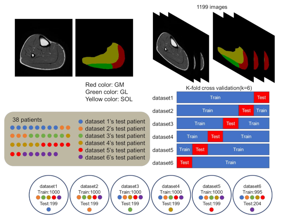
These images were saved as PNG images by dividing the triceps into three classes (GM, GL, and SOL) with an in-house MATLAB software; the regions of interest (ROIs) were also manually defined (Figure 2). The ROIs were manually defined by the author alone and were then verified by two radiological technologists with 5 (T.Y.) and 20 years of experience (H.S.), respectively. A total of 1199 images were prepared from 38 patients, and the Train:Test was set to 10:2. The 38 patients were classified into six groups, and six datasets were created so that one could be used as a test (Figure 2). Six different datasets with 1199 images were prepared for K-fold cross-validation so that the number of tests would be approximately 200. Data augmentation for improving the training [6] was performed on the training images, and they were rotated by 5° from −45 to 45°, increasing the number of images by 19 times.

2.4. Training for Creating Models

The software was developed with MATLAB software, and a computer with NVIDIA GeForce GTX 1080Ti 12GB (NVIDIA Corporation, Santa Clara, CA, USA) was used. DeepLabv3+ was used for the architecture for implementation of image segmentation models. The model was inputted with 2D images taken by MRI. The following training parameters were used: the batch size for the number of training samples was 32, the number of epochs was 100, and the initial learning rate was 0.0001. Using this network model, six different datasets were trained to create six models.

2.5. Interpolation

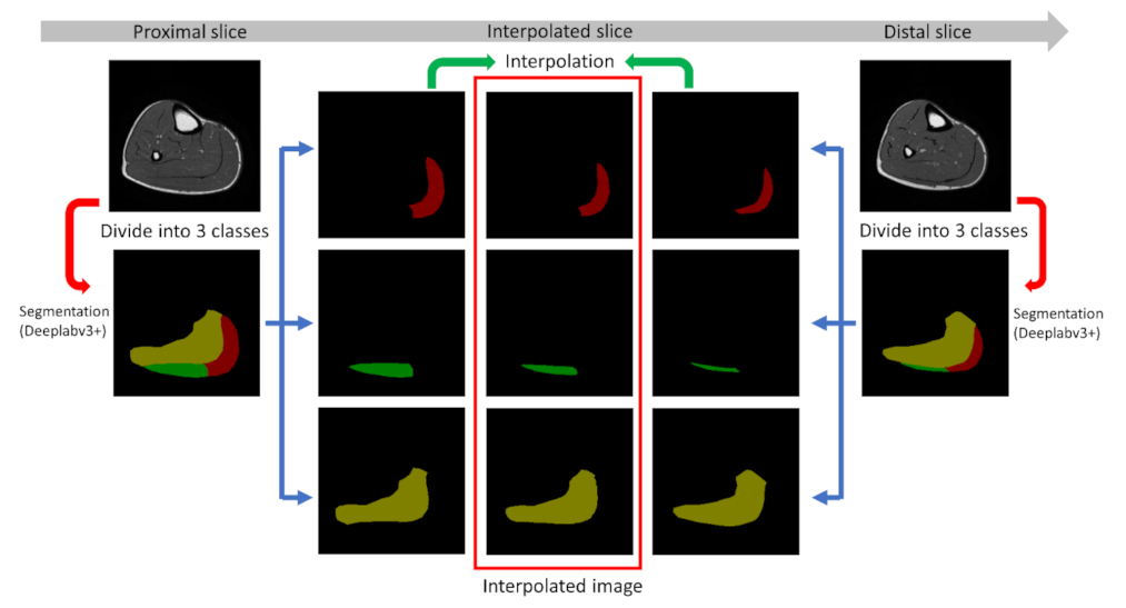
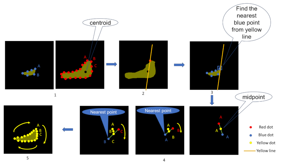
The supervised images and the images generated using the devised model were divided in each patient and classified into three muscle types (GM, GL, and SOL). Only the images with muscles present in the supervised images were extracted and interpolated by excluding even-numbered images from the predicted images in the same position (Figure 3 and Figure 4). The interpolation method is described in Figure 5. Interpolation was performed in the slice direction from two images of the muscle. The contours of the two muscles were represented by points. The centroid of the larger muscle was calculated and connected to the centroid by a point on the larger muscle. The distance between the connecting line and all points on the smaller muscle was calculated, and the point with the smallest distance was adopted. Moreover, the midpoint was calculated by connecting the adopted point to a point on the larger muscle. The same process was performed for all points of the larger muscle, and by connecting all the calculated midpoints, the interpolated image of the muscle was completed.

2.6. Indicators Used for Evaluation

2.6.1. DSC

When the supervised images were set as A and the predicted images were set as B, the following formula was used to calculate DSC. This value is an index to check the agreement between the images, and the closer the value is to 1, the better the agreement is.
D S C   =   2   ×   A     B A   +   B

2.6.2. Calculation of the Volume and Error Rate

The spacing between the slices and pixels were obtained from the DICOM data. The number of pixels used in the labeled muscle was determined, and the volume was calculated from the product of these values. The error rate was calculated to compare the volume of the supervised images with that of the predicted images. The error rate was calculated using the following formula.
V o l u m e   o f   p r e d i c t e d   i m a g e s     V o l u m e   o f   s u p e r v i s e d   i m a g e s V o l u m e   o f   s u p e r v i s e d   i m a g e s   ×   100   %  

2.7. Evaluation of the Created Models

DSCs were calculated for each muscle using the abovementioned formula, and the averages were calculated for each dataset to show the overall average. All images were used for this evaluation. The volumes were calculated for each patient and muscle, and the average error rates of the datasets were calculated using the mentioned formula. For this evaluation, only the images with muscle present in both the supervised and predicted images were used to calculate the error rate.

2.8. Evaluation of the Interpolation Method

Only the interpolated images were used to obtain DSCs, and the average DSC for each muscle was calculated. DSCs were calculated from the interpolated image and the supervised image of the same number (Figure 4C). The volumes were calculated from the interpolated images, and the error rates were calculated for comparison with the volumes of the supervised images. To confirm that the interpolation method is useful in terms of reducing volumetric errors, the error rate was calculated by comparing the volume of the supervised image and the volume of the image with the spacing between its slices doubled without interpolation while excluding even numbered images (Figure 4D). All patients with all three muscles and all predicted images that could be interpolated were used for these evaluations. Statistical tests were performed to compare the interpolated and supervised volumes. First, the Shapiro–Wilk test was applied to evaluate normality; if normality was accepted, the t-test was used; otherwise, the Wilcoxon signed-ranked test, a nonparametric test, was used. The differences in the statistical analyses were considered statistically significant when p was <0.05.

3. Results

3.1. Evaluation of the Created Models

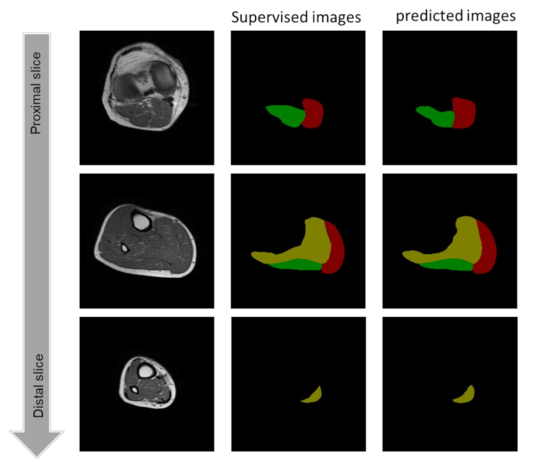
The DSC values per dataset are shown in Table 2. The following table shows the DSC values of all 67 leg muscles. GM and SOL were detected with relatively high accuracy. However, the DSCs of GL were lower than those of the others. The following are some representative examples of segmentation successes and failures (Figure 6 and Figure 7)
The error rates of volume per dataset are shown in Table 3. The following table shows the error rates of the volumes of all 67 legs that were present in the supervised and predicted images. The total error represents the error rate of all three muscle volumes. The error rate of MG, SOL, and sum was 10% but that of the GL volume was large.

3.2. Evaluation of the Interpolation Method

The DSC values of the interpolated images are shown in Table 4. The following table shows the DSC of 60 GMs, 54 GLs, and 66 SOLs in the interpolated images. All muscles had mean DSC larger than 0.8.
The error rates of volume for the interpolated images are shown in Table 5. The following table shows the error rate between the volume of the supervised images (Figure 4A) and the volume calculated from the 52 legs to which all the three muscles could be interpolated (Figure 4C). For GM, SOL, and the total error, the percentage was <10%. In fact, the percentage of the total error was as low as 7.5%. The usefulness of this interpolation method in reducing volume calculation errors was evaluated by comparing the error rate between the volume of the supervised image (Figure 4A) and the volume of the non-interpolated image (Figure 4D). In the comparison between the supervised and non-interpolated muscles, all muscles were >12%. Both volumes were calculated for each leg and were then statistically tested. p value results showed that there were no significant differences between the volumes of the supervised and interpolated muscles. the same sequence for the supervised and non-interpolated muscle were performed, and the p value results also showed that there were no significant differences.

4. Discussion

With regards to the evaluation of the created models, DSCs were used to compare the agreement of the images and evaluate whether the detection was correct in the two dimensions. Based on the results of the evaluation of the created models, MG and SOL were detected with higher accuracy than GL, with DSCs exceeding 0.8. As for MG and SOL, the DSC of segmentation in the thigh muscle, which exceeded 0.8 in many previous studies, were found to be lower than the respective values in DSCs, but the values themselves cannot be compared because the target areas were different. However, this study could detect MGs with a higher accuracy than the reported segmentation of MGs without using deep learning [22]. For GM and SOL, there were many large muscles present, but there were some false positives, which were detected with a DSC of >0.8 on average. As for the DSCs of GL, GL was shorter in the craniocaudal direction than the other two muscles, and the number of slices in which GL exists is small. The slices at the edge of the GLs were so small that it was difficult for the human eye to recognize them, and the ratio of the number of small GLs slices was higher than that of other muscles. In small muscles where the other muscles and surrounding fat tissues are mistakenly detected as GL, false positives were more common and this was believed to be the cause of the decline in DSCs. Figure 7 is a representative example of partially incorrectly predicted images. Not only are there false detections of the SOL as the GL and GM, but there are also examples of inaccurate location. As per Ding’s study [17], when false positives, which were not present in the surveillance images, appeared in the prediction images, DSC was zero and affected the average DSC. In addition, some images used in the test were blurry, and false positives were particularly common in these. The triceps surae is a long muscle that exists in a craniocaudal direction, and the shape of the muscle changes, particularly at the level of the knee and calf. In this study, the number of slices was uneven in each position; therefore, the number of slices at the knee level was small, which affected DSCs. As there were no reports on the segmentation of the triceps surae, the results were compared with those of the quadriceps. In a study by Kemnitz et al. [16], using T1-weighted 250 images of thighs, including the quadriceps, hamstrings, sutures, adductor muscles, and others, were prepared and trained with U-Net, which reported a muscle-only DSC of >0.9. However, as this was only a result for a specific anatomical location, it may not be suitable for the volume calculation and interpolation that were performed in this study. In a report by Ding et al. [17], 46 thigh 4968-slice Fat-water decomposition MRI images were trained with U-Net. The mean DSC of the quadriceps, hamstrings, sutures, and thin muscles was 0.89, and the mean percent difference in volume was 7.57%. A similar study was conducted to determine DSC and error rates for different image types and regions used; the results showed a similar trend to the present study, indicating the validity of the present results. With regards to volumetry without interpolation, the agreement was represented in three dimensions by calculating the error rates of the volume.
Based on the average error rates of volumes per dataset, the error rate of GM, SOL, and sum was 10%. The error rate in the GL volume was large, probably due to the presence of many false positives as in DSC. In addition, the predicted images were overestimated in all muscles, which might be due to the false positives because they were surrounded by other muscles and fat. Of the images used for training, the images with all three muscles present were the most common; however, there were few images at the level of the knee where only the gastrocnemius muscle was present, and the quadriceps muscles were mistakenly detected as gastrocnemius. In addition, images with contrast and roughness were also detected that made it difficult to see the boundaries between the muscles, and false positives were frequent in these images.
The interpolation method was evaluated in-plane by calculating the DSC of the supervised and interpolated images. All muscles had mean DSC larger than 0.8. The evaluation of Table 4 was DSC evaluated only with interpolated images; hence, it can be said that the interpolation was performed with high accuracy. In this interpolation method, the centroid of the larger muscle contour was discovered, and the centroid was connected to the dots that make up the contour; the dot with the shortest distance between the line and that of the smaller muscle contour were adopted. If a dot in the false positive area was adopted, the DSC was lowered. Even if they were not considered in this interpolation, all of them were >0.8, so the correct dot with a higher probability among the corresponding dots in the small contour was selected. In a study by Yap Abdullah et al. [23], the results of an interpolation to measure the intracranial volume were comparable to those of manual segmentation, and its use led to the development of a software for rapid measurement. In a study by Nordez et al. [24], to calculate the volume of the quadriceps muscle in MRI images, four different methods were used to calculate the error rate; it was reported that the interpolation method was the best. These results using the interpolation method showed the same trend as these studies.
The interpolation method was evaluated along the slice direction by calculating and comparing the error rates of muscle volumes, including the supervised and interpolated images. The volume contained interpolated images generated from the two images but with low error rates. Therefore, the results in Table 5 demonstrate that the interpolation method is effective in reducing the volumetric error. The percentages of GM, SOL, and total errors were >10%; for the total error, the percentage was as low as 7.5% because if there were no false positives in the images before and after the interpolated images, there were no false positives in the interpolated images. This was believed to lead to a decreased error rate because of the possibility of reduced false positives. Even if false positives existed, it seemed that the probability of adopting dots that constitute false positives was low. There was no significant difference between the volumes of the supervised and interpolated images, indicating that this method can be used without any problems in calculating the volume. From the results in Table 4 and Table 5, interpolation was performed by excluding the even numbered images from the subsequent evaluation. As these findings underline that the interpolation was accomplished with high accuracy, while observing at the same time the effect of volume reduction, the error with the actual volume could be further reduced by interpolating the actual captured images that were found.
This study has some limitations. First, this study was unable to interpolate all images used in the test. Because muscles were present in the supervised images and the even number of those present in the predicted images were excluded, if the muscles were small in the supervised images, they could not be detected and the images could not be complemented. Therefore, the solution is to improve the detection capability by training more images or to prepare a test image where the number of interpolatable images exists. Second, the error rate of the volume calculated in this study could not be calculated in the legs without gastrocnemius or SOL muscles. Therefore, to get a more correct error rate, it would be necessary to have all the three muscle types in the legs used for training or testing. Third, most studies on quadriceps segmentation used U-Net [16,17,18]. In these studies [25,26], network models were compared for segmentation, and deeplabv3puls was shown to have the highest detection ability. Therefore, DeepLabv3+ was used for segmentation instead of U-Net because Deeplabv3+, which has a higher detection capability, was more likely to be able to detect muscles with higher accuracy than U-net. Using this algorithm, the triceps could be detected immediately and determine its volume. However, the recent advances in the channel and spatial attention mechanisms [27,28,29] have definitely led to the evolution of semantic segmentation using U-Net. Therefore, a further study on CNNs in the state of the art is needed. Fourth, the hyperparameters were not adjusted because this study did not aim to tune the hyperparameters as in the study by Chieh et al. [30]. Setting and training the optimal hyperparameters may lead to more accurate detection with Bayesian Optimization. Fifth, the sample size of data is small. Not only is it difficult to guarantee generalization performance with small sample size, but it is also possible to improve accuracy by increasing sample size. Additionally, in this study, training and test images were divided 10:2 for six-fold cross validation, but five- or ten-fold is general [31,32]. This value was obtained by dividing the data by person, and it is thought that cross-validation can be performed with general values by increasing the sample size. Sixth, there are no studies of triceps surae muscle segmentation using Deep Learning. Therefore, this study was compared with a study of quadriceps segmentation [15,16,17,18,19,20] and a study of triceps surae muscle segmentation that did not use deep learning [21]. The results showed that the DSC of the quadriceps was higher than the DSC of this study, which suggests that this study has room for DSC improvement. In addition, it was more accurate than the reported segmentation of the triceps surae muscle. This interpolation method can be used to calculate their volume without any problems found. Although muscle perimeter length and cross-sectional area, which are correlated with muscle volume [33,34], are sometimes used as indices, it is more accurate to calculate volume from images of the entire muscle [35]. However, it is more accurate to calculate the volume from the whole muscle image. Therefore, this study, which can calculate the actual volume by immediately calculating the volume and interpolating between slices, suggests the possibility of advancing research in the field of physical therapy. The technique of detecting the triceps and calculating their volume can be used to other parts and organs, and it was assumed that the interpolation method can be used to determine the volume more accurately. The interpolation technique may also be useful in smoothing out the images captured with a thicker slice for multiplanar reconstruction processing and 3D visualization.

5. Conclusions

This deep learning segmentation technique could detect the triceps with relatively high DSCs. This eliminates the time needed to manually identify the muscles, and thus enables us to immediately calculate the respective volume. The ability to immediately calculate the volume of the triceps muscle will provide a distinct contribution to research studies in the field of physical therapy, including the ability to immediately perform the quantitative evaluations of rehabilitation devices in leg muscles. The interpolation method used in this study to determine the volume was useful. Using the interpolation method allowed us to find that the difference between the volume calculated by the interpolation method and the actual measurement could be smaller than the volume calculated solely from the captured image. In the future, this interpolation method can be used to calculate the volume of other muscles and organs as well, thereby making it possible to calculate the respective volume in a more accurate manner.

Author Contributions

Y.A. contributed to the data analysis, algorithm construction, and the writing and editing of the manuscript. T.Y. (Takaaki Yoshimura), K.M. and T.Y. (Tomonari Yamada) reviewed and edited the manuscript. H.S. proposed the idea and contributed to the data acquisition, performed supervision, project administration, and reviewed and edited the paper. All authors have read and agreed to the published version of the manuscript.

Funding

This research received no external funding.

Institutional Review Board Statement

The study was conducted according to the guidelines of the Declaration of Helsinki and approved by the Hokkaido University Hospital.

Informed Consent Statement

Informed consent was waived because of the retrospective nature of the study and the analysis used anonymous clinical data.

Data Availability Statement

The created models in this study are available on request from the corresponding author. However, the image datasets presented in this study are not publicly available due to ethical reasons, e.g., because they contain sensitive information that could compromise the privacy of the participants. The source code of this study is available at https://github.com/MIA-laboratory/TricepsMRIsegmentation (accessed on 7 December 2021).

Acknowledgments

The authors would like to thank the laboratory members of the Medical Image Analysis laboratory and Yoshimura’s laboratory for their help. The authors would also like to thank Masayuki Kugimoto for providing us with useful advice and information.

Conflicts of Interest

The authors declare that no conflict of interest exist.

References

  1. Son, S.; Jeong, Y.; Lee, B. An audification and visualization system (AVS) of an autonomous vehicle for blind and deaf people based on deep learning. Sensors 2019, 19, 5053. [Google Scholar] [CrossRef] [Green Version]
  2. Chen, Y.; Aggarwal, P.; Choi, J.; Jay, C.C. A deep learning approach to drone monitoring. In Proceedings of the 2017 Asia-Pacific Signal and Information Processing Association Annual Summit and Conference (APSIPA ASC), Kuala Lumpur, Malaysia, 12–15 December 2017; pp. 686–691. [Google Scholar] [CrossRef] [Green Version]
  3. Ghaderi, A.; Sanandaji, B.M.; Ghaderi, F. Deep Forecast: Deep Learning-based Spatio-Temporal Forecasting. In Proceedings of the International Conference on Machine Learning, Time Series Workshop, Sydney, NSW, Australia, 6–11 August 2017. [Google Scholar]
  4. Silver, D.; Schrittwieser, J.; Simonyan, K.; Antonoglou, I.; Huang, A.; Guez, A.; Hubert, T.; Baker, L.; Lai, M.; Bolton, A.; et al. Mastering the game of Go without human knowledge. Nature 2017, 550, 354–359. [Google Scholar] [CrossRef]
  5. Sugimori, H.; Hamaguchi, H.; Fujiwara, T.; Ishizaka, K. Classification of type of brain magnetic resonance images with deep learning technique. Magn. Reson. Imaging 2021, 77, 180–185. [Google Scholar] [CrossRef]
  6. Sugimori, H.; Kawakami, M. Automatic detection of a standard line for brain magnetic resonance imaging using deep learning. Appl. Sci. 2019, 9, 3849. [Google Scholar] [CrossRef] [Green Version]
  7. Zhou, X. Automatic Segmentation of Multiple Organs on 3D CT Images by Using Deep Learning Approaches. Adv. Exp. Med. Biol. 2020, 1213, 135–147. [Google Scholar] [CrossRef] [PubMed]
  8. Yang, S.; Kweon, J.; Roh, J.H.; Lee, J.H.; Kang, H.; Park, L.J.; Kim, D.J.; Yang, H.; Hur, J.; Kang, D.Y.; et al. Deep learning segmentation of major vessels in X-ray coronary angiography. Sci. Rep. 2019, 9, 16897. [Google Scholar] [CrossRef]
  9. Zhang, L.; Mohamed, A.A.; Chai, R.; Guo, Y.; Zheng, B.; Wu, S. Automated deep learning method for whole-breast segmentation in diffusion-weighted breast MRI. J. Magn. Reson. Imaging 2020, 51, 635–643. [Google Scholar] [CrossRef] [PubMed]
  10. Kessler, D.A.; MacKay, J.W.; Crowe, V.A.; Henson, F.M.D.; Graves, M.J.; Gilbert, F.J.; Kaggie, J.D. The optimisation of deep neural networks for segmenting multiple knee joint tissues from MRIs. Comput. Med. Imaging Graph. 2020, 86, 101793. [Google Scholar] [CrossRef] [PubMed]
  11. Cattagni, T.; Scaglioni, G.; Laroche, D.; Gremeaux, V.; Martin, A. The involvement of ankle muscles in maintaining balance in the upright posture is higher in elderly fallers. Exp. Gerontol. 2016, 77, 38–45. [Google Scholar] [CrossRef]
  12. Belavý, D.L.; Miokovic, T.; Rittweger, J.; Felsenberg, D. Estimation of changes in volume of individual lower-limb muscles using magnetic resonance imaging (during bed-rest). Physiol. Meas. 2011, 32, 35–50. [Google Scholar] [CrossRef]
  13. Tortorella, C.; Simone, O.; Piazzolla, G.; Stella, I.; Cappiello, V.; Antonaci, S. Role of phosphoinositide 3-kinase and extracellular signal-regulated kinase pathways in granulocyte macrophage-colony-stimulating factor failure to delay fas-induced neutrophil apoptosis in elderly humans. J. Gerontol. Ser. A 2006, 61, 1111–1118. [Google Scholar] [CrossRef]
  14. Karamanidis, K.; Epro, G.; König, M.; Mersmann, F.; Arampatzis, A. Simplified Triceps Surae Muscle Volume Assessment in Older Adults. Front. Physiol. 2019, 10, 1299. [Google Scholar] [CrossRef] [Green Version]
  15. Friedberger, A.; Figueiredo, C.; Bäuerle, T.; Schett, G.; Engelke, K. A new method for quantitative assessment of hand muscle volume and fat in magnetic resonance images. BMC Rheumatol. 2020, 4, 72. [Google Scholar] [CrossRef] [PubMed]
  16. Kemnitz, J.; Baumgartner, C.F.; Eckstein, F.; Chaudhari, A.; Ruhdorfer, A.; Wirth, W.; Eder, S.K.; Konukoglu, E. Clinical evaluation of fully automated thigh muscle and adipose tissue segmentation using a U-Net deep learning architecture in context of osteoarthritic knee pain. Magn. Reson. Mater. Phys. Biol. Med. 2020, 33, 483–493. [Google Scholar] [CrossRef] [PubMed] [Green Version]
  17. Ding, J.; Cao, P.; Chang, H.C.; Gao, Y.; Chan, S.H.S.; Vardhanabhuti, V. Deep learning-based thigh muscle segmentation for reproducible fat fraction quantification using fat–water decomposition MRI. Insights Imaging 2020, 11, 128. [Google Scholar] [CrossRef]
  18. Gadermayr, M.; Li, K.; Müller, M.; Truhn, D.; Krämer, N.; Merhof, D.; Gess, B. Domain-specific data augmentation for segmenting MR images of fatty infiltrated human thighs with neural networks. J. Magn. Reson. Imaging 2019, 49, 1676–1683. [Google Scholar] [CrossRef] [PubMed]
  19. Ghosh, S.; Ray, N.; Boulanger, P. A Structured Deep-Learning Based Approach for the Automated Segmentation of Human Leg Muscle from 3D MRI. In Proceedings of the 2017 14th Conference on Computer and Robot Vision (CRV), Edmonton, AB, Canada, 16–19 May 2017; pp. 117–123. [Google Scholar] [CrossRef]
  20. Andrews, S.; Hamarneh, G. The Generalized Log-Ratio Transformation: Learning Shape and Adjacency Priors for Simultaneous Thigh Muscle Segmentation. IEEE Trans. Med. Imaging 2015, 34, 1773–1787. [Google Scholar] [CrossRef] [PubMed] [Green Version]
  21. Baudin, P.-Y.; Azzabou, N.; Carlier, P.G.; Paragios, N. Automatic Skeletal Muscle Segmentation through Random Walks and Graph-Based Seed Placement. In Proceedings of the 2012 9th IEEE International Symposium on Biomedical Imaging (ISBI), Barcelona, Spain, 2–5 May 2012; pp. 1036–1039. [Google Scholar] [CrossRef] [Green Version]
  22. Essafi, S.; Langs, G.; Deux, J.F.; Rahmouni, A.; Bassez, G.; Paragios, N. Wavelet-driven knowledge-based MRI calf muscle segmentation. In Proceedings of the 2009 IEEE International Symposium on Biomedical Imaging: From Nano to Macro, Boston, MA, USA, 28 June–1 July 2009; pp. 225–228. [Google Scholar] [CrossRef]
  23. Abdullah, J.Y.; Rajion, Z.A.; Martin, A.G.; Jaafar, A.; Ghani, A.R.I.; Abdullah, J.M. Shape-based interpolation method in measuring intracranial volume for pre- and post-operative decompressive craniectomy using open source software. Neurocirugia 2019, 30, 115–123. [Google Scholar] [CrossRef]
  24. Nordez, A.; Jolivet, E.; Südhoff, I.; Bonneau, D.; De Guise, J.A.; Skalli, W. Comparison of methods to assess quadriceps muscle volume using magnetic resonance imaging. J. Magn. Reson. Imaging 2009, 30, 1116–1123. [Google Scholar] [CrossRef]
  25. Ahmed, I.; Ahmad, M.; Khan, F.A.; Asif, M. Comparison of deep-learning-based segmentation models: Using top view person images. IEEE Access 2020, 8, 136361–136373. [Google Scholar] [CrossRef]
  26. Khan, Z.; Yahya, N.; Alsaih, K.; Ali, S.S.A.; Meriaudeau, F. Evaluation of deep neural networks for semantic segmentation of prostate in T2W MRI. Sensors 2020, 20, 3183. [Google Scholar] [CrossRef]
  27. Rundo, L.; Han, C.; Nagano, Y.; Zhang, J.; Hataya, R.; Militello, C.; Tangherloni, A.; Nobile, M.S.; Ferretti, C.; Besozzi, D.; et al. USE-Net: Incorporating Squeeze-and-Excitation blocks into U-Net for prostate zonal segmentation of multi-institutional MRI datasets. Neurocomputing 2019, 365, 31–43. [Google Scholar] [CrossRef] [Green Version]
  28. Schlemper, J.; Oktay, O.; Schaap, M.; Heinrich, M.; Kainz, B.; Glocker, B.; Rueckert, D. Attention gated networks: Learning to leverage salient regions in medical images. Med. Image Anal. 2019, 53, 197–207. [Google Scholar] [CrossRef]
  29. Yeung, M.; Sala, E.; Schönlieb, C.-B.; Rundo, L. Focus U-Net: A novel dual attention-gated CNN for polyp segmentation during colonoscopy. Comput. Biol. Med. 2021, 137, 104815. [Google Scholar] [CrossRef] [PubMed]
  30. Chen, L.C.; Zhu, Y.; Papandreou, G.; Schroff, F.; Adam, H. Encoder-decoder with atrous separable convolution for semantic image segmentation. In Lecture Notes in Computer Science; Springer: Berlin/Heidelberg, Germany, 2018; pp. 833–851. [Google Scholar] [CrossRef] [Green Version]
  31. Do, D.T.; Le, T.Q.T.; Le, N.Q.K. Using deep neural networks and biological subwords to detect protein S-sulfenylation sites. Brief. Bioinform. 2021, 22, bbaa128. [Google Scholar] [CrossRef]
  32. Le, N.Q.K.; Huynh, T.T. Identifying SNAREs by Incorporating Deep Learning Architecture and Amino Acid Embedding Representation. Front. Physiol. 2019, 10, 1501. [Google Scholar] [CrossRef] [PubMed]
  33. Miyachi, R.; Yamazaki, T.; Ohno, N.; Miyati, T. Relationship between muscle cross-sectional area by mri and muscle thickness by ultrasonography of the triceps surae in the sitting position. Healthcare 2020, 8, 166. [Google Scholar] [CrossRef] [PubMed]
  34. Henninger, H.B.; Christensen, G.V.; Taylor, C.E.; Kawakami, J.; Hillyard, B.S.; Tashjian, R.Z.; Chalmers, P.N. The Muscle Cross-sectional Area on MRI of the Shoulder Can Predict Muscle Volume: An MRI Study in Cadavers. Clin. Orthop. Relat. Res. 2020, 478, 871–883. [Google Scholar] [CrossRef] [PubMed]
  35. Akagi, R.; Takai, Y.; Ohta, M.; Kanehisa, H.; Kawakami, Y.; Fukunaga, T. Muscle volume compared to cross-sectional area is more appropriate for evaluating muscle strength in young and elderly individuals. Age Ageing 2009, 38, 564–569. [Google Scholar] [CrossRef] [Green Version]
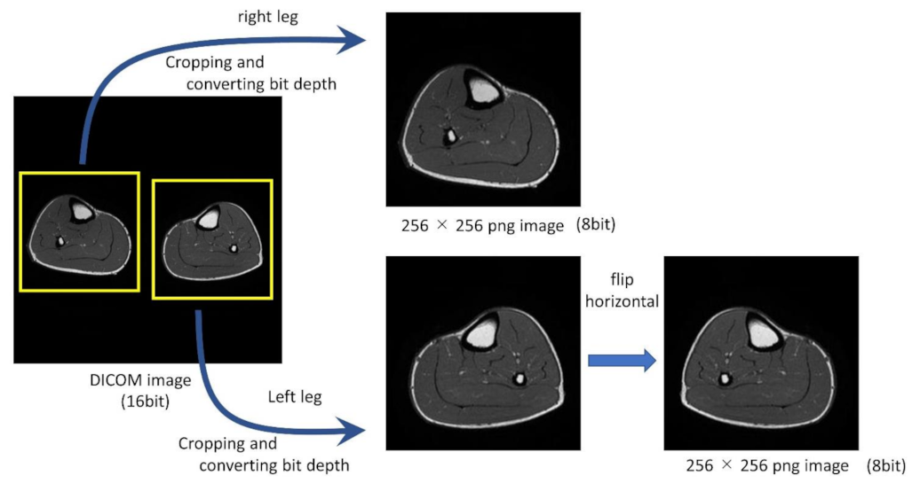
Figure 1. The conversion process from DICOM to PNG image.
Applsci 11 12006 g001
Figure 2. Six divided datasets and 6-fold cross-validation.
Applsci 11 12006 g002
Figure 3. Classifying muscles into three for interpolation.
Applsci 11 12006 g003
Figure 4. Creating the interpolated images from the predicted images based on the presence or absence of muscles in the supervised images. (A) Muscles in supervised images; (B) Predictive muscles using segmentation model; (C) Interpolated muscles using the interpolation method by thinning out the even number of predicted images; (D) Muscles with even-numbered predicted images thinned out and slice thickness doubled without using the interpolation method; 1–9; The number of the slice where the muscle is located.
Applsci 11 12006 g004
Figure 5. Procedure of interpolation: (1) The outline with dots and the calculated centroid of the muscle with the most dots were expressed; (2) a line was drawn connecting the red dot and the centroid; (3) measured the distance between all the blue points and the yellow line, found the nearest blue point from yellow line; (4) the midpoint of the red dot and the selected blue dot was marked; (5) a different red dot was selected and steps 2 through 4 were repeated for as many red dots as there are red dots, connecting all the yellow dots.
Applsci 11 12006 g005
Figure 6. Representative examples of accurately predicted images.
Applsci 11 12006 g006
Figure 7. Representative examples of partially incorrectly predicted images.
Applsci 11 12006 g007
Table 1. The details information of the obtained images (N = 38).
Mean ± SD [Min–Max]
Number of slices17.9 ± 4.9 [3–29]
Field of view [ mm ]342.1 × 295.0 [160 × 160–500 × 425]
Acquisition matrix size [pixel]446.0 × 402.4 [320 × 224–672 × 672]
Pixel size [ mm ]0.764 × 0.764 [0.559 × 0.559–0.928 × 0.928]
Slice thickness [ mm ]5.8 ± 0.5 [4–6]
Slice gap [ mm ]13.6 ± 4.7 [4.8–22.8]
Length of acquisition [ mm ]231.0 ± 76.2 [42–342]
Table 2. Average DSC values per dataset for the predicted images.
PositionDataset1Dataset2Dataset3Dataset4Dataset5Dataset6Mean ± SD
GM0.8970.7540.8760.8300.7760.7450.813 ± 0.064
GL0.8040.5910.7650.7730.6390.7040.713 ± 0.084
SOL0.8890.8200.7910.8230.8400.8440.835 ± 0.033
GM: gastrocnemius medialis, GL: gastrocnemius lateralis, SOL: soleus, SD: standard deviation.
Table 3. The error rate of volume per dataset for the predicted images.
PositionDataset1Dataset2Dataset3Dataset4Dataset5Dataset6Mean ± SD
GM5.6811.848.9610.288.8024.4811.67 ± 6.60
GL27.4623.0318.7427.1432.7112.3623.57 ± 7.22
SOL11.7117.2214.606.875.929.2410.93 ± 4.43
total error11.0713.3811.877.277.8412.4310.64 ± 2.51
[%], GM: gastrocnemius medialis, GL: gastrocnemius lateralis, SOL: soleus, SD: standard deviation.
Table 4. The DSC values of the interpolated images.
PositionDSC
GM0.877 ± 0.134
GL0.809 ± 0.170
SOL0.867 ± 0.078
GM: gastrocnemius medialis, GL: gastrocnemius lateralis, SOL: soleus, DSC: Dice similarity coefficient.
Table 5. The error rate of volume for the interpolated images.
Comparison TargetPositionError Rate [%]p Value
Supervised muscle and interpolated muscleGM9.41 ± 7.650.5052
GL17.89 ± 6.370.3098
SOL9.43 ± 5.070.7280
total error7.69 ± 3.49-
Supervised muscle and non-interpolated muscleGM20.28 ± 9.680.1499
GL33.93 ± 7.540.2539
SOL12.70 ± 5.790.3442
total error14.97 ± 3.98-
GM: gastrocnemius medialis; GL: gastrocnemius lateralis; SOL: soleus. Supervised muscle: Figure 4A; interpolated muscle: Figure 4C; non-interpolated muscle: Figure 4D.
Publisher’s Note: MDPI stays neutral with regard to jurisdictional claims in published maps and institutional affiliations.