Abstract
Accurate and stable load forecasting has great significance to ensure the safe operation of distributed energy system. For the purpose of improving the accuracy and stability of distributed energy system load forecasting, a forecasting model in view of kernel principal component analysis (KPCA), kernel extreme learning machine (KELM) and fireworks algorithm (FWA) is proposed. First, KPCA modal is used to reduce the dimension of the feature, thus redundant input samples are merged. Next, FWA is employed to optimize the parameters C and σ of KELM. Lastly, the load forecasting modal of KPCA-FWA-KELM is established. The relevant data of a distributed energy system in Beijing, China, is selected for training test to verify the effectiveness of the proposed method. The results show that the new hybrid KPCA-FWA-KELM method has superior performance, robustness and versatility in load prediction of distributed energy systems.
1. Introduction
The concept of energy internet will effectively promote world energy production, consumption and system reform, and drive energy transformation in all countries so as to achieve energy cleanliness, efficiency, safety, convenience, and sustainable use [1]. As an important component of energy internet, distributed energy system (DES) has attracted widespread attention due to its outstanding features for instance safety and re-liability, high energy efficiency, environmental friendliness, and sustainability [2]. However, the use of distributed energy (DE) has malpractices such as random output. Therefore, precise prediction of space-time load of DES has great significance owing to the assistance of improving the overall stability of the system operation and promoting the effective use of distributed energy.
For years, with the advancement of mathematical theory and the rapid development of modern computer technology, the technology and methods of load forecasting are developing all the time, which mainly includes classical prediction method and modern intelligent prediction method. Traditional prediction methods, which include time series method [3], regression analysis method [4], grey theory method [5] and so on, is simple and mature. However, due to certain defects, the prediction accuracy is unsatisfactory. Analysis of the time series method ignores the influence of other external factors on account of taking time factors as the only variable. Consequently, there will be a serious error in the prediction results when the external environment changes greatly [6]. The regression prediction method belongs to a speculate when choosing the explanatory variable or the way that the explanatory variable is expressed, which affects the diversity of the explanatory variables and the intractability of some explanatory variables to a certain extent, so as to cause the regression analysis method to be limited in predicting the load of DES [7]. The grey prediction method has a great fitting effect on the raw data as a smooth discrete sequence [8]. In contrast, the date of influencing factors of DES load are discrete. Thus, the accuracy of prediction will be greatly reduced by using grey prediction method. In summary, classical prediction method is not suitable for load forecasting of DES.
Currently, scholars gradually applied intelligent algorithms into load forecasting as the emergence of various algorithms. Since intelligent algorithms can simulate the human brain mechanism, simulation forecast the change of objects through the function of self-learning and self-optimization, establish suitable models, the prediction accuracy of intelligent algorithms such as artificial neural network (ANN) has been improved [9]. Due to these elements, scholars began to focus on continuous optimization of ANN and support vector machine (SVM), so as to enhance the convergence speed and the accuracy of the prediction results. Zeng, et al. took full account of the weather factors and established a short-term load prediction method in view of back propagation neural network (BPNN) which is a typical representative of ANN algorithm [10]. Gwo-Ching proposed a load prediction model in view of improvement differential evolution (IDE) and wavelet neural network (WNN) [11]. The ANN model can be used to control the error in a small range, however, this kind of algorithm converges slowly and is likely to fall into local optimum. Therefore, for the local optimization of neural networks, some scholars use support vector machine (SVM) for load forecasting research [12]. Based on SVM, Abdoos et al. [13] and Barman et al. [14] established load prediction models which promoted the prediction accuracy compared with the BPNN model. In contrast, for large-scale training samples, SVM is hard to achieve, and it is hard to solve the multi-classification problem [15].
As a new feedforward neural network, extreme learning machine (ELM), which overcome the defects of traditional BPNN and SVM, has been applied in a number of prediction areas and has obtained more accurate prediction results [16,17,18] for reducing the risk of falling into the local optimality. Since ELM has poor predict stability because of the characteristics of random initialization of inputting weight and hidden layer offset, Guangbin Huang et al. [19] introduced a kernel extreme learning machine (KELM) algorithm, which overcomes the weakness of poor stability of ELM and improves the learning accuracy of the algorithm. However, the performance of KELM is easily affected by the penalty coefficient C and the kernel parameter σ, therefore KELM needs to be solved by intelligent algorithms for parameter optimization with regard to the problems of difficult selection for these two parameters. The inspiration of fireworks algorithm comes from the explosion of air fireworks, which is a new type of swarm intelligence algorithm with global optimization solution of explosive search mechanism, shows great accuracy and high efficiency when solving complex optimization problems [20]. Thus, FWA to be selected for optimizing the parameters of KELM in this paper.
It is worth noting that the load forecasting of DES has a number of influence factors if all load factors are employed as the input characteristics of the prediction method, there will be a great number of factors due to the strong coupling, non-linearity, and information redundancy among factors [21]. Therefore, it is also important to reduce the dimension of input features. Principal component analysis (PCA) has a preferable treatment effect as a multivariate statistical method to synthesize multiple variables into a few variables, when it is dealing with various indicators with strong linear relationships [22]. On the other hand, factors that affect load changes in distributed energy systems, such as humidity, cloudiness, barometric pressure, and temperature, are non-linear in most cases [23]. However, as a linear method, PCA, which cannot obtain the high-order characteristics of the data and ignores the nonlinear information of the data while reducing the dimension. As a result, this paper uses kernel principal component analysis (KPCA) [24] to map the initial input variables to the high-dimensional feature space through nonlinear transformation and reduce the dimensionality of the input variables while preserving nonlinear information between the input variables.
In summary, this study preliminarily established the feature set of candidate influence factors of distributed energy system load and builds a distributed energy system load prediction model based on KPCA and FWA algorithm to optimize KELM. The other parts of this article are arranged as follows. The next part introduces the algorithm of this article, including kernel principal component analysis, FWA algorithm and KELM model, and constructs a complete prediction framework. The third part selects the practical cases to verify the effectiveness and stability of the proposed method. The fourth part is the conclusion.
2. Basic Theory
2.1. KPCA
As a nonlinear principal component model, KPCA which can get more reasonable result of index reduction compared with PCA, can effectively solve the nonlinear relationship among variables, and is effectively used in multi-index comprehensive analysis [25]. This method can compress the information contained in a great quantity of index variables into a few comprehensive variables that can reflect the original information features. In addition, by analyzing the index of the inclusive variables, it can process the nonlinear relationship between the variables and minimize the loss of the original data information [26]. The basic steps are as follows [27,28].
We set a combination of random vectors containing N random variables, thereinto, , and m stands for the input sample size. That is: the initial input sample data set is . By projecting to the space through nonlinear mapping, the dataset is projected to: , and it satisfies .
Get the covariance matrix according to the definition of covariance:
Solve:
Get it’s the eigenvalue and the eigenvector, wherein is an eigenvalue; is the feature vector which is corresponding to the eigenvalue.
Get by matrix centralization:
wherein, is n × n the matrix, satisfy simultaneously Ii, j = 1/n, the Formula (3) is simplified to:
After the above calculation, we can use the method of principal component analysis in traditional PCA to calculate the projection of a data point on the eigenvector, and finally the kernel principal component of the point can be obtained.
2.2. Improved Fireworks Model
FWA is the simulation of the whole fireworks explosion process [29]. Fireworks exploded to make sparks, the sparks make more new sparks at the same time, so as to constitute rich patterns. Converting the process of fireworks explosion into the calculation process of FWA, fireworks to be seen as feasible solutions of the problem, and the process of spark generation is understood as the process of finding the optimal result. In the process of solving the optimal solution, the influencing factors of FWA include the number of sparks, the blast radius, and a best group of fireworks and sparks which the next explosion selects.
FWA has a self-regulation mechanism with good local search and global search capabilities. In FWA, the explosion radius and explosion spark quantity of each firework is dissimilar. Fireworks with a larger explosion radius and a poor fitness value give fireworks more “ability to explore”-exploration ability. While the firework with a good fitness value owns a smaller explosion radius, enabling it to have a greater “ability of excavation” -exploitability around the location. Furthermore, the introduction of Gaussian mutation sparks can further enrich the diversity of a population.
Therefore, it can be seen that the three main components of FWA are explosion operator, mutation operator and selection strategy.
(1) Explosion operator. According to fitness value of fireworks, the amount of spark and explosion radius produced by each fireworks explosion can be obtained. The calculation formulas of spark number Si and explosion radius Ai are as follows towards the fireworks xi (I = 1, 2, …, N).
In Formulas (7) and (8), , denote the maximum and minimum fitness value of the current population respectively; the fitness value of the fireworks denotes expressed in ; and adjusts the quantity of explosive sparks as a constant; in addition, indicates that the size of the fireworks explosion radius is set to a constant; moreover, in order to avoid zero operation, is used as the minimum machine value.
(2) Mutation operator. Mutation operator can add the variety of the spark population. The variation spark in FWA is the Gaussian mutation sparks created by the explosion sparks through Gaussian mutation. When selecting fireworks , the k-dimensional Gaussian mutation exercise is used as: ; thereinto, represents k-dimensional variation spark, and indicates that it conforms to Gaussian distribution.
In FWA, when the explosion spark and mutation spark generated by the operator are separated from the search space, it must to map them to a new location, the calculation method is as follows:
wherein, , denote the upper and lower search spaces on the k-dimension.
(3) Selection strategy. A certain number of individuals need to be selected for the next generation of fireworks in explosion fireworks and mutation sparks so as to information for future generations of fireworks.
Candidates with the best fitness value will become the next generation of fireworks when individuals are selected and is population’s number. For the remaining fireworks, the choice is made in a probabilistic way. For fireworks , the calculation method is as follows:
wherein, represents the sum of the distances between all samples in the current individual candidate set. In set, the probability that a sample is selected will decrease when the individual has a higher density, which it also means there are other candidates around this individual.
Based on the previous description, the specific process of FWA method is obtained [30]:
Step 1. Initialize parameters, randomly select N fireworks in the solution space, and initialize its coordinates.
Step 2. Calculate the fitness value for each firework and calculated their explosion radius and spark number . Randomly select the coordinate in to update the coordinates.
Step 3. Firstly, Gaussian abrupt spark is generated; Then selecting the spark , calculating the result of Gaussian mutation sparks based on Gaussian mutation formula, and save them to the population of Gaussian mutation sparks.
Step 4. The probability formula is aimed to select the best individual from the fireworks, explosion sparks and Gaussian mutation sparks as the next iteration fireworks.
Step 5. Determine the termination condition. If the termination condition is not met, continue the loop until the best result is output; if it meets, the cycle ends.
2.3. KELM
Huang et al. put forward the theory of extreme learning machine in 2006. On account of this theory, many scholars have innovated in addition to a variety of models, such as online sequential extreme learning machine and KELM [31,32]. KELM is a single-layer feedforward neural network algorithm, which is more accurate than the extreme learning machine (ELM) algorithm. Compared with BPNN and SVM, the kernel function extreme learning machine has shorter time to calculate results, faster calculation speed, and greatly improves the adaptability of the model to the samples [33]. KELM algorithm has been effectively applied in many fields, which proves its effectiveness in prediction.
The following introduces the construction principle of the general ELM model, and the specific neural network function is as follows:
In the formula: g (x) denotes the output value of the network, hi (x) represents the output of the i hidden layer neurons corresponding to the input x; represents the connection weights between the i hidden layer neurons and the output neurons.
The regression accuracy of ELM is measured by the error. The smaller the error is, the greater the accuracy is. Therefore, the minimum output error is calculated to obtain the optimal result. The formula is as follows:
In the formula, L represents the quantity of hidden layer neurons; represents the function to be forecasted composed of the target value.
The generalization ability of neural networks is measured by minimizing the output weight β. Usually β takes its least squares solution, the calculation method is as follows:
In the formula: H represents the hidden layer matrix of neural network; represents the generalized inverse matrix of H matrix; O represents the prediction target value vector. On the basis of ridge regression theory, by improving the normal number 1/C, the results will be more stable with better generalization.
The introduction of kernel function to KELM algorithm can obtain better regression prediction accuracy. This paper uses Mercer’ s condition to define the kernel matrix, and the calculation formula is as follows:
Kernel matrix replaces random matrix HHT in ELM and uses kernel function to map all input samples from n-dimensional space to high-dimensional hidden feature space. After setting the kernel parameters, the mapping value of the kernel matrix is fixed [33]. The kernel function includes RBF kernel function, linear kernel function and polynomial kernel function, which is usually set as RBF kernel function:
The parameter 1/C is added to the main diagonal of the unit diagonal matrix HHT, so that the characteristic root will not be equal to zero, and then the weight vector β* is obtained. A more stable and better generalization ELM model is obtained. At this time the output weights of ELM method become [34]:
In the formula, I denotes diagonal matrix; C denotes penalty coefficient for weighing the proportion between structural risk and empirical risk; HHT denotes generated by mapping input samples from kernel functions.
From the above formulas, the output of the KELM model is described as follows:
In the kernel KELM algorithm, it is not necessary to give the specific form of the feature mapping function h(x) of the hidden layer node, and the output value can be gotten only by knowing the specific form of the kernel function [35]. Furthermore, so the kernel function is directly in the form of inner product, it is not necessary to set the number of hidden layer nodes, nor to set the initial weight and bias of hidden layer.
2.4. Model Construction
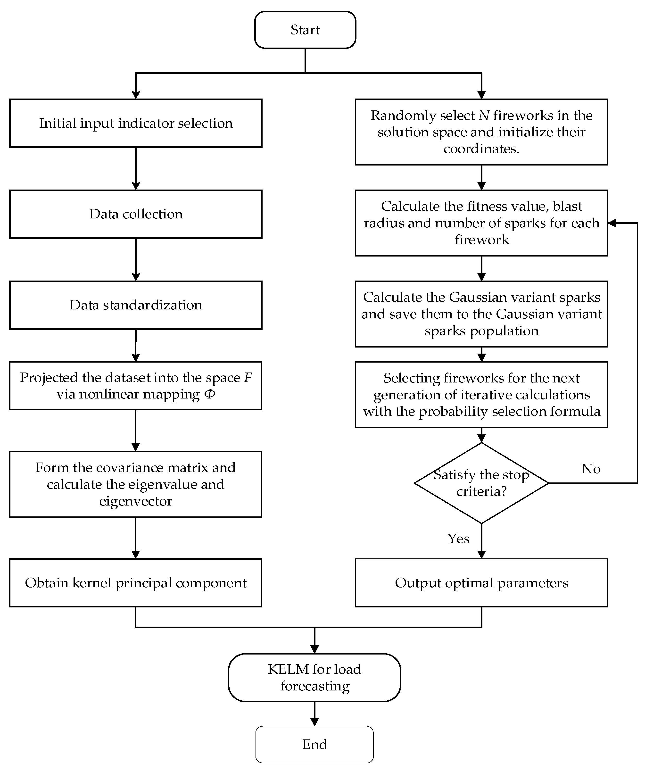
This paper first determines the feature set of the candidate influence factors of the distributed energy system and uses KPCA method to deal with the feature dimensionality reduction, and then uses the fireworks algorithm to optimize the KELM, thus the optimal value of the penalty coefficient C and the kernel parameter σ is obtained. Finally, the characteristic data after KPCA reduction are input to get the prediction result. The proposed composite prediction framework is shown in Figure 1.
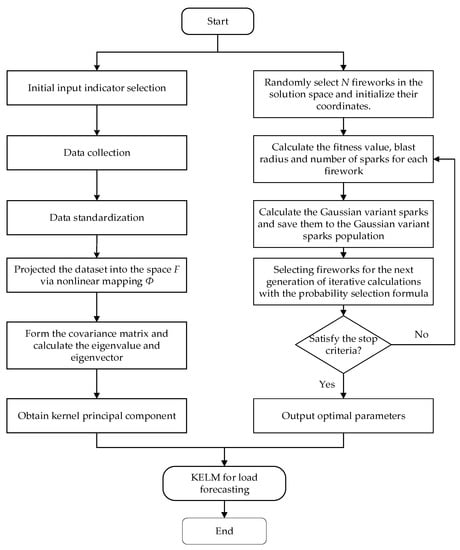
Figure 1.
The proposed composite prediction framework.
The following are the specific steps of the prediction model.
- (1)
- Initial input variable selection and data processing. The influence factors of the distributed energy system load are determined by the literature data analysis, and the candidate input variables C = {Ci, i = 1, 2, …, n} are formed, and quantify and normalize the input data (Ci).
- (2)
- KPCA feature reduction. After step (1), a matrix is formed based on the input data, the nonlinear mapping function selects the Gauss kernel function . After the KPCA nonlinear transformation in the Section 2.1, the kernel principal component is retained when the cumulative variance contribution rate is greater than 90 %, and finally a new input variable matrix is formed.
- (3)
- Initialize the FWA parameter. After many tests, the maximum quantity of iterations is , the quantity of population is , the quantity of spark determines the constant , and the radius of explosion determines the constant .
- (4)
- Get the best values of C and σ in KELM. Firstly, C and σ will be randomly assigned, and then the fitness of each generation will be compared to select the best parameters. Judge whether each iteration satisfies the stop condition of the algorithm. If yes, the parameter is the global optimal parameter. If not, start a new cycle until the global optimal parameter is found.
- (5)
- Simulation prediction. According to the prediction model above, the short-term load of distributed energy system is forecasted, and the results of load forecasting are analyzed and evaluated.
3. Error Measures
It is very important to find the model with the best prediction effect among many models, and the indexes to evaluate the advantages and disadvantages of prediction models usually include: relative error (RE), root mean square error (RMSE), average absolute error (MAPE) and average absolute error (AAE). The smaller the error value, the better the accuracy of prediction, and the more effective the method. The calculation formula of these four indicators are as follows:
In the formula, represents the actual charge at time t, denotes the predicted charge at time t, and N represents the data group.
4. Case Study and Results Analysis
4.1. Data Selection and Pretreatment
For the sake of verify the forecasting accuracy of the method, this paper selects the load data and meteorological data of the distributed energy system in China from 0:00 on 18 June 2018 to 24:00 on 18 June 2019. The charge data from 0:00 on 14 June 2018 to 24:00 on 14 June 2019 are selected as training samples to establish univariate time series. The charge data from 0:00 on 18 June 2019 to 24:00 on 18 June 2019 are utilized as testing sample, with the information collection frequency being 15 min. Simultaneously, the maximum temperature, average temperature, minimum temperature, season type, month, precipitation regime, day type, wind speed, humidity, and the load value at the same time in the previous five days are considered as the candidate set for feature selection, totaling 30 candidate features, as shown in Table 1.

Table 1.
The whole candidate features.
Since the collected data is not public, the main statistical indicators are listed in Table 2.

Table 2.
The main statistical indicators of the collecting data.
For the better training and learning of the proposed model, all input data should be normalized:
In the formula, represents the actual value, denotes the minimum value of the sample, denotes the maximum value, and denotes the standardized load.
Furthermore, KPCA is adopted to make principal component analysis of 30 reference vectors and extract 4 sets of vectors as the input vector of the proposed model.
4.2. KELM for Load Forecasting
After the dimensionality reduction of input features, input parameters are brought into the KELM model for learning. In this article, the self-programming program is utilized to the operation in Matlab software. It is It is noteworthy that RBF kernel function is selected in the article as the kernel function of KELM method. To ensure its precision and accuracy, the model’s important parameters are obtained and optimized by FWA algorithm. The parameters of FWA algorithm are set in Section 2.4, hence they are not repeated here. Through calculation, the KELM model parameters are C = 8.325 and σ = 0.0031.
For the sake of proving the forecasting accuracy of the proposed DES load forecasting method, this paper also selects the KELM, ELM and BPNN which are not optimized by FWA to forecast the load data of this sample, and then evaluates and analyzes the prediction results of the four methods. The structure of the BPNN model is 6-3-1, whose hidden layer transfer function is expressed as “tansig” function, while the output layer transfer function is expressed as purelin function, with the maximum time of training being 300, the minimum error of training objectives being 0.0001, the rate of training being 0.1, and the original weight and threshold values derived from the model’s own learning. In the ELM method, the penalty parameter obtained from training C is 10.276 and the kernel parameter σ is 0.0013. In the KELM model parameters, C is 10.108 and σ is 0.0026.
Table 3 shows the DES load prediction results of BPNN, ELM, KELM, and the method proposed in the article on the test set.

Table 3.
Partial predicted and actual values of the test set (Unit: kW).
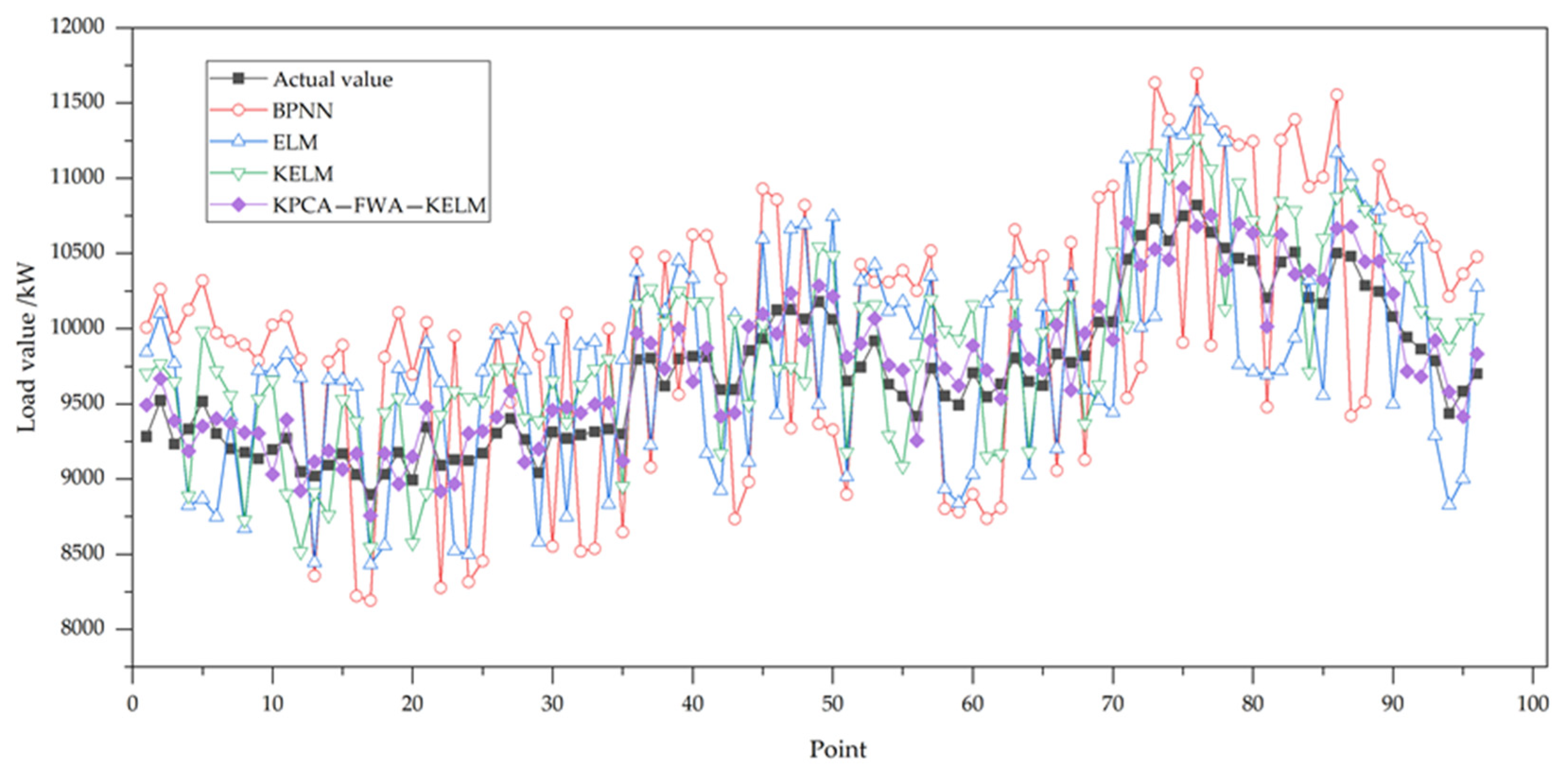
In order to intuitively analyze, the predicted results in Table 3 are drawn into diagrams, as shown in Figure 2. It can be found from Table 3 and Figure 2 that the predicted results of the four methods are not very different from the real data, and the overall trend is consistent. Among them, the prediction results of KPCA-FWA-DIR method are most similar to the actual situation, and the prediction results of other models have relatively large errors. Furthermore, the results show that the prediction curve of KELM method is more accurate than that of single prediction curve, indicating that the introduction of kernel function increases the accuracy of the model to a certain extent.
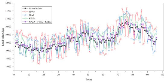
Figure 2.
Prediction results.
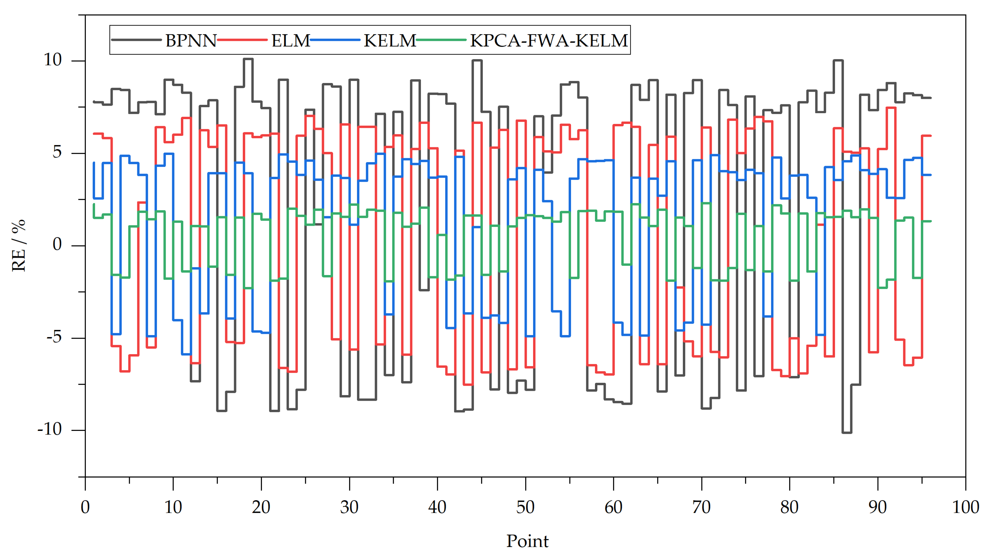
Figure 3 shows the relative errors of the four methods. By observing Figure 4, we can clearly see the differences in the forecasting results of different models.
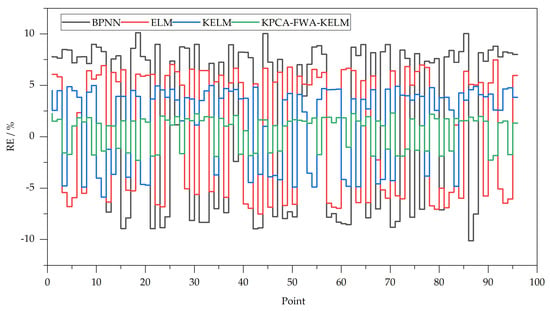
Figure 3.
RE of prediction results.

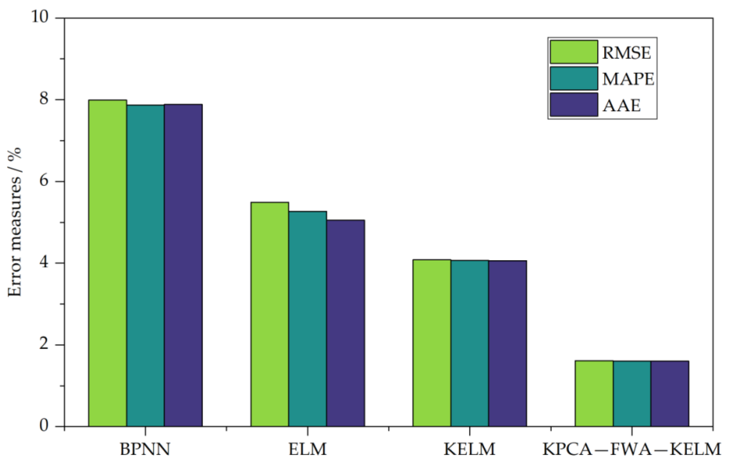
Figure 4.
RMSE, MAPE and AAE of the prediction results.
The RE ranges [−3%, 3%] and [−1%, 1%] are usually used as standards to measure the accuracy of forecasting methods. As shown in Figure 4, the forecasting errors at all time points of the KPCA-FWA-KELM model are not only in the [−3%, 3%] interval, but also within [−2.5%, 2.5%]. The minimum value of the relative error absolute values is 0.58% and the maximum value is 2.31%, of which only 8 sample points have errors outside [−2%, 2%], which are sample points with serial numbers 1, 19, 31, 39, 63, 71, 79 and 91, respectively. The relative errors are 2.25%, −2.29%, 2.23%, 2.06%, 2.24%, 2.31%, 2.19% and −2.28%, respectively. In the KELM prediction method, the relative error of 11 prediction results is controlled in within [−3%, 3%]. The error of the three prediction results is within [−1.5%, 1.5%], in which the serial numbers are 13, 31 and 45 respectively. Their relative errors are −1.22%, 1.15% and 1.01% respectively. The minimum absolute value of relative error is 1.01% and the maximum is 5.89%. In the ELM model, the error of 4 sample points is controlled in within [−3%, 3%], which are the samples of the sequence number of 7, 68 and 84 respectively. The relative errors are 2.35%, −2.26% and 1.14%, respectively, but they are all outside the [−1%, 1%] range. Its minimum of the absolute value of the relative error is 1.14% and the maximum value is 7.52%. The minimum value of absolute relative error of BPNN method is 1.16%, and the maximum is 10.12%. The error of most prediction results is in [−9%, −7%] and [7%, 9%], and the fluctuation range is large. From this point of view, the KPCA-FWA-KELM method has the best prediction effect, followed by KELM method and ELM method, and BPNN method has the worst effect. It can be found that KPCA-FWA-KELM modal has the best prediction accuracy and stability, which shows that FWA algorithm improves the ability of model learning, effectively avoids the problem of falling into local optimization, and improves the global search ability of KELM. It is also shown that the prediction results obtained from the KPCA model can achieve satisfactory prediction results and effectively eliminate the interference of redundant data. Furthermore, ILSSVM has better performance than LSSVM, SVM and BPNN. This result shows that LSSVM can achieve better prediction effect after improvement.
The RMSE, MAPE and AAE of BPNN, ELM, KELM and KPCA-FWA-KELM are shown in Figure 4. We can find that the RMSE, MAPE and AAE of the proposed methods are 1.6158%, 1.6079% and 1.6017% respectively, which are the least error of the above five methods. Furthermore, errors of RMSE, MAPE and AAE of KELM methods are 4.0873%, 4.0713% and 4.0649% respectively. The RMSE, MAPE and AAE of ELM method were 5.4899%, 5.2693% and 5.0553% respectively. RMSE, MAPE and AAE of the BPNN method are 7.9917%, 7.8731% and 7.8878% respectively.
These indexes reflect the overall error of model forecasting and the degree of error discretization. Therefore, it can be further seen that the overall forecasting effect of the KELM method is superior to the ELM method and the BPNN method, while the overall forecasting effect of the ELM method is superior to the BPNN method, indicating that the overall forecasting performance of the ELM method is significantly improved after the introduction of the kernel function. The forecasting effect of the KPCA-FWA-KELM method is better than that of the KELM method. Practice has proved that using FWA algorithm to select KELM method C and σ can obtain better optimization effect, while KPCA method can reduce redundant data while ensuring the integrity of input information, so as to achieve ideal forecasting effect.
In summary, the method proposed in this article optimizes the KELM method by the FWA algorithm and obtains the appropriate parameters C and σ in the KELM method, which can effectively decrease the load forecasting error.
On the one hand, KPCA method can ensure the integrity of input information, on the other hand, it can decrease the noise in the input variables to enhance the effectiveness of input variables, so as to enhance the accuracy and stability of distributed energy system load prediction. The data calculation results prove the effectiveness and stability of the load prediction method proposed in this article.
5. Conclusions
This paper puts forward a hybrid load prediction method that combines KPCA with KELM optimized by FWA. First, for the sake of forecasting the power load of DES, the KPCA method is used to select input features. In addition, the FWA method is employed to optimize the parameters of KELM. Lastly, after the optimized input subset and the best values of C and σ are obtained, the method is used for load prediction of DES. The following results are obtained through this study.
- (1)
- KPCA can effectively decrease the influence of non-correlation noise and improve the prediction performance.
- (2)
- The introduction of FWA optimization algorithm can enhance the global search ability, and the KELM method optimized by FWA shows good results.
- (3)
- On the basis of the error index, in comparison with ELM, KELM has achieved better prediction results, indicating that the method of improving ELM by introducing kernel function is effective (RMSE, MAPE and AAE are respectively 4.0873%, 4.0713% and 4.0649%). Therefore, the KPCA-FWA-KELM load prediction modal proposed in this paper is effective and feasible and is expected to become an effective alternative method for load prediction in power industry.
Author Contributions
Conceptualization, Y.L.; methodology, H.W.; software, H.W.; validation, H.W.; formal analysis, Y.F.; investigation, Y.L.; resources, H.W.; data curation, X.Z.; writing—original draft preparation, Y.F. and H.W.; writing—review and editing, Q.Y. and Y.L.; visualization, Y.F.; supervision, Y.L.; project administration, Y.L.; funding acquisition, Y.L. All authors have read and agreed to the published version of the manuscript.
Funding
This work is supported by Science Foundation of Ministry of Education of China (Project No. 21YJC630072), Natural Science Foundation of Hebei Province, China (Project No. G2020403008) and the Fundamental Research Funds for the Universities in Hebei Province, China (Project No. QN202210).
Conflicts of Interest
The authors declare no conflict of interest.
References
- Sani, A.S.; Yuan, D.; Bao, W.; Dong, Z.J. A Universally Composable Key Exchange Protocol for Advanced Metering Infrastructure in the Energy Internet. IEEE Trans. Ind. Inform. 2020, 17, 534–546. [Google Scholar] [CrossRef]
- Wu, Z.; Yao, J.; Zhu, P.; Yang, F.; Meng, X.; Kurko, S.; Zhang, Z. Study of MW-scale biogas-fed SOFC-WGS-TSA-PEMFC hybrid power technology as distributed energy system: Thermodynamic, exergetic and thermo-economic evaluation. Int. J. Hydrogen Energy 2021, 46, 11183–11198. [Google Scholar] [CrossRef]
- Kocak, C.; Dalar, A.Z.; Yolcu, O.C.; Bas, E.; Egrioglu, E. A new fuzzy time series method based on an ARMA-type recurrent Pi-Sigma artificial neural network. Soft Comput. 2020, 24, 8243–8252. [Google Scholar] [CrossRef]
- Wang, P.; Zhou, Y.; Sun, J. A new method for regression analysis of interval-censored data with the additive hazards model. J. Korean Stat. Soc. 2020, 49, 1131–1147. [Google Scholar] [CrossRef]
- Jia, Y.; Li, G.; Dong, X.; He, K. A novel denoising method for vibration signal of hob spindle based on EEMD and grey theory. Measurement 2021, 169, 108490. [Google Scholar] [CrossRef]
- Akdi, Y.; Gölveren, E.; Ünlü, K.D.; Yücel, M.E. Modeling and forecasting of monthly PM2.5 emission of Paris by periodogram-based time series methodology. Environ. Monit. Assess. 2021, 193, 1–15. [Google Scholar] [CrossRef]
- Wang, Y.; Jia, P.; Cui, H.; Peng, X. A novel regression prediction method for electronic nose based on broad learning system. IEEE Sens. J. 2021, 21, 17. [Google Scholar] [CrossRef]
- Duan, H.; Pang, X. A Multivariate Grey Prediction Model Based on Energy Logistic Equation and Its Application in Energy Prediction in China. Energy 2021, 229, 120716. [Google Scholar] [CrossRef]
- Herzog, S.; Tetzlaff, C.; Wrgtter, F. Evolving artificial neural networks with feedback. Neural Netw. 2020, 123, 153–162. [Google Scholar] [CrossRef]
- Zeng, Y.R.; Zeng, Y.; Choi, B.; Wang, L. Multifactor-Influenced Energy Consumption Forecasting Using Enhanced Back-propagation Neural Network. Energy 2017, 127, 381–396. [Google Scholar] [CrossRef]
- Gwo-Ching, L. Hybrid Improved Differential Evolution and Wavelet Neural Network with load forecasting problem of air conditioning. Int. J. Electr. Power Energy Syst. 2014, 61, 673–682. [Google Scholar]
- Shankar, K.; Lakshmanaprabu, S.K.; Gupta, D.; Maseleno, A.; De Albuquerque, V.H.C. Optimal feature- based multi- kernel SVM approach for thyroid disease classification. J. Supercomput. 2020, 76, 1–16. [Google Scholar] [CrossRef]
- Abdoos, A.; Hemmati, M.; Abdoos, A.A. Short term load forecasting using a hybrid intelligent method. Knowl. Based Syst. 2015, 76, 139–147. [Google Scholar] [CrossRef]
- Barman, M.; Choudhury, N.B.D.; Sutradhar, S. A regional hybrid GOA-SVM model based on similar day approach for short-term load forecasting in Assam, India. Energy 2018, 145, 710–720. [Google Scholar] [CrossRef]
- Wang, H.; Liang, Y.; Ding, W.; Niu, D.; Li, S.; Wang, F. The Improved Least Square Support Vector Machine Based on Wolf Pack Algorithm and Data Inconsistency Rate for Cost Prediction of Substation Projects. Math. Probl. Eng. 2020, 2020, 1–14. [Google Scholar]
- Shamsah, S.; Owolabi, T.O. Modeling the Maximum Magnetic Entropy Change of Doped Manganite Using a Grid Search-Based Extreme Learning Machine and Hybrid Gravitational Search-Based Support Vector Regression. Crystals 2020, 10, 310. [Google Scholar] [CrossRef]
- Zhang, T.; Tang, Z.; Wu, J.; Du, X.; Chen, K. Multi-Step-Ahead Crude Oil Price Forecasting Based on Two-layer Decomposition Technique and Extreme Learning Machine Optimized by the Particle Swarm Optimization Algorithm. Energy 2021, 229, 120797. [Google Scholar] [CrossRef]
- Liang, Y.; Niu, D.; Cao, Y.; Hong, W.-C. Analysis and Modeling for China’s Electricity Demand Forecasting Using a Hybrid Method Based on Multiple Regression and Extreme Learning Machine: A View from Carbon Emission. Energies 2016, 9, 941. [Google Scholar] [CrossRef] [Green Version]
- Zhou, Y.; Peng, J.; Chen, C. Extreme Learning Machine with Composite Kernels for Hyperspectral Image Classification. IEEE J. Sel. Top. Appl. Earth Obs. Remote Sens. 2017, 8, 2351–2360. [Google Scholar] [CrossRef]
- Wang, P.; Zhang, N. Real-time detection of burst faults of key nodes in optical transmission networks based on fireworks algorithm. Int. J. Sens. Netw. 2020, 33, 98. [Google Scholar] [CrossRef]
- Vieira, D.; Silva, B.E.; Menezes, T.V.; Lisboa, A. Large scale spatial electric load forecasting framework based on spatial convolution. Int. J. Electr. Power Energy Syst. 2020, 117, 105582. [Google Scholar] [CrossRef]
- Chen, X.; Wang, L.; Huang, Z. Principal Component Analysis Based Dynamic Fuzzy Neural Network for Internal Corrosion Rate Prediction of Gas Pipelines. Math. Probl. Eng. 2020, 2020, 1–9. [Google Scholar] [CrossRef]
- Borii, A.; Torres, J.; Popov, M. Fundamental study on the influence of dynamic load and distributed energy resources on power system short-term voltage stability. Int. J. Electr. Power Energy Syst. 2021, 131, 107141. [Google Scholar]
- Lahdhiri, H.; Taouali, O. Reduced Rank KPCA based on GLRT chart for sensor fault detection in nonlinear chemical process. Measurement 2020, 169, 108342. [Google Scholar] [CrossRef]
- Liang, Y.; Niu, D.; Hong, W.-C. Short Term Load Forecasting Based on Feature Extraction and Improved General Regression Neural Network model. Energy 2019, 166, 653–663. [Google Scholar] [CrossRef]
- Zhang, Y.; Lin, Z.; Lin, X.; Zhang, X.; Zhao, Q.; Sun, Y. A gene module identification algorithm and its applications to identify gene modules and key genes of hepatocellular carcinoma. Sci. Rep. 2021, 11, 5517. [Google Scholar] [CrossRef] [PubMed]
- Long, Z.; Zhou, X.; Wu, X. Cascaded Approach to Defect Location and Classification in Microelectronic Bonded Joints: Improved Level Set and Random Forest. IEEE Trans. Ind. Inform. 2019, 16, 4403–4412. [Google Scholar] [CrossRef]
- Sumner, J.; Alaeddini, A. Analysis of Feature Extraction Methods for Prediction of 30-Day Hospital Readmissions. Methods Inf. Med. 2019, 58, 213–221. [Google Scholar] [CrossRef]
- Liu, F.; Xiao, B.; Li, H. Finding Key Node Sets in Complex Networks Based on Improved Discrete Fireworks Algorithm. J. Syst. Sci. Complex. 2021, 34, 1014–1027. [Google Scholar] [CrossRef]
- Qiao, Z.; Ke, L.; Zhang, G.; Wang, X. Adaptive collaborative optimization of traffic network signal timing based on immune-fireworks algorithm and hierarchical strategy. Appl. Intell. 2021, 51, 6951–6967. [Google Scholar] [CrossRef]
- Li, W.; Meng, J.E.; Shi, Z. A Kernel Extreme Learning Machines Algorithm for Node Localization in Wireless Sensor Networks. IEEE Commun. Lett. 2020, 24, 1433–1436. [Google Scholar]
- Chen, S.; Gu, C.; Lin, C.; Wang, Y.; Hariri-Ardebili, M.A. Prediction, Monitoring, and Interpretation of Dam Leakage Flow via Adaptative Kernel Extreme Learning Machine. Measurement 2020, 166, 108161. [Google Scholar] [CrossRef]
- Wang, Z.; Chen, S.; Guo, R.; Li, B.; Feng, Y. Extreme learning machine with feature mapping of kernel function. IET Image Process. 2020, 14, 2495–2502. [Google Scholar] [CrossRef]
- Sharma, E.; Deo, R.C.; Prasad, R.; Parisi, A.V. A hybrid air quality early-warning framework: An hourly forecasting model with online sequential extreme learning machines and empirical mode decomposition algorithms. Sci. Total Environ. 2020, 709, 135934. [Google Scholar] [CrossRef]
- Liu, Y.; Fang, J.J.; Shi, G. Calibration of magnetic compass using an improved extreme learning machine based on reverse tuning. Sens. Rev. 2019, 39, 121–128. [Google Scholar] [CrossRef]
Publisher’s Note: MDPI stays neutral with regard to jurisdictional claims in published maps and institutional affiliations. |
© 2021 by the authors. Licensee MDPI, Basel, Switzerland. This article is an open access article distributed under the terms and conditions of the Creative Commons Attribution (CC BY) license (https://creativecommons.org/licenses/by/4.0/).

