Inverse Approach of Parameter Optimization for Nonlinear Meta-Model Using Finite Element Simulation

Abstract

Accurate and efficient estimation and prediction of the nonlinear behavior of materials during plastic working is a major issue in academic and industrial settings. Studies on property meta-models are being conducted to estimate and predict plastic working results. However, accurately representing strong nonlinear properties using power-law and exponential models, which are typical meta-models, is difficult. The combination meta-model can be used to solve this problem, but the possible number of parameters increases. This causes a cost problem when using FE simulation. In this study, the accuracy of the nonlinear properties of materials and the number of iterations were compared for three typical meta-models and the proposed advanced meta-models considering stress–strain properties. A material property test was conducted using ASTM E8/E8M, and the meta-model was initialized using ASTM E646 and MATLAB Curve Fitting Toolbox. A finite element (FE) simulation was conducted for the meta-models, and the test and simulation results were compared in terms of the engineering stress–strain curve and the root-mean-square error (RMSE). In addition, an inverse method was applied for the FE simulation to estimate the true stress–strain properties, and the results were analyzed in terms of the RMSE and the number of iterations and simulations. Finally, the need for an advanced meta-model that exhibits strong nonlinearity was suggested.

1. Introduction

The number of safety and environmental problems encountered in the construction and automotive industries is continuously increasing [1,2]. Therefore, the utilization of lightweight materials and high-strength materials for user safety is increasing [3,4]. However, part design and plastic working for such high-strength materials become difficult owing to the nonlinear properties resulting from hardening during plastic working. A typical method for identifying the nonlinear properties of materials is a tensile test, and tensile test results can be expressed using a force–displacement graph. This graph is then converted to an engineering stress–strain curve [5]. During this process, the curve can be transformed into a true stress–strain curve, which reflects the changes in the cross-sectional area, using an extrapolation, interpolation, or regression method [6,7,8,9,10,11]. An extrapolation, interpolation, or regression model is used as a meta-model in the form of a constitutive equation to simulate the test data. A property meta-model (typically called a material model, hardening model, etc.), which is an approximate model that accounts for practical physical phenomena, is widely used in engineering design and optimization processes. Property meta-models are used to represent elastic and plastic properties against the strength of materials [12]. In general, elastic properties are expressed by a linear function such as the Hook model, whereas plastic properties are expressed by power-law, exponential, and combination models [13,14,15,16,17,18,19]. When a curve-fit meta-model is applied to a finite element (FE) simulation, an engineering stress–strain curve is obtained, along with the differences between the FE simulation results and the actual test results. Thus, the inverse method is being investigated to reduce the differences between these results by applying a meta-model for the FE simulation in order to obtain the true stress–strain curve [20,21,22]. The inverse method is a meta-model-based optimization process that searches for the optimal property values by repeatedly performing FE simulations and updating the parameters of a meta-model to reduce errors. For the inverse method, nonlinear models such as power-law and exponential models can be considered as property meta-models. In addition, a modified meta-model such as a combination model can be considered to represent the nonlinear properties of high-strength, large-strain materials [23,24,25,26]. These meta-models are being researched to increase the order or term for representing nonlinear properties [27,28]. When the parameters of a meta-model increase, the resources and costs required by the inverse method increase. Therefore, a meta-model that exhibits a higher accuracy with a smaller number of parameters than that used for the typical meta-models is required.

To compare the estimated performance of the properties for different meta-models, this study compared the RMSE values, the number of iterations, and the sum of FE simulations of the typical meta-models with those of the proposed advanced meta-model corresponding to the plastic property of high-strength materials. First, the engineering stress–strain curves were obtained by conducting ASTM E8/E8M [29] uniaxial tensile tests for 10705MBU, a high-strength metal. Then, curve fitting was performed for the true stress–strain curves of three typical property meta-models (i.e., Gosh, Hockett–Sherby, and combination meta-models) and the advanced meta-models (Gaussian mixture, sum of sine, and polynomial). The MATLAB Curve Fitting Toolbox (CFT) was used for the parameter initializing process. In addition, HyperMesh was used for FE modeling and LS-DYNA for FE simulations. The property meta-models applied to the FE simulation were optimized using LS-OPT. The simulation and optimization results were compared in terms of the RMSE values and the iteration of convergence. Finally, the proposed advanced meta-models were determined to have an advantage over the typical property meta-models for estimating the nonlinear behaviors of high-strength metals.

2. Preprocess

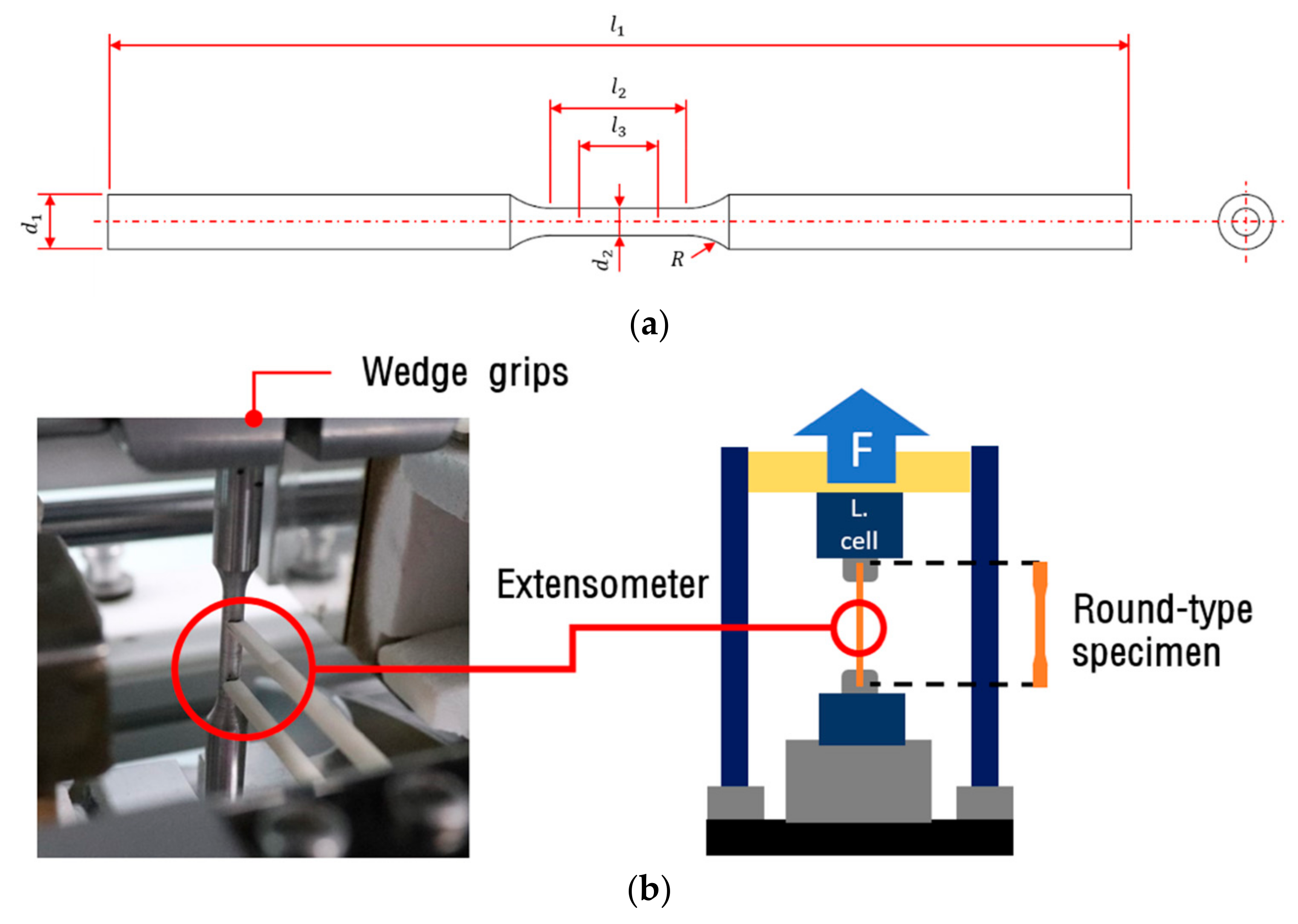
2.1. Experimental Material, Procedure

The test material considered in this study is high-strength stainless steel 10705MBU, which is often used in forging. The number of specimens used in this tensile test is three, and their dimensions are presented in

Table 1. Nominal dimensions of specimen.

Symbol	Description	Dimensions [mm]
$l_1$	Length overall	150
$l_2$	Length of narrow section	20
$l_3$	Gage length	12
$d_1$	Diameter of grip section	8
$d_2$	Diameter of narrow section	4
$R$	Radius of fillet	10

and Figure 1. Specimens with a circular cross-section were used in this study to minimize the anisotropic effect [30,31].

The tensile test was conducted in accordance with the provisions of ASTM E8/E8M. Using the universal testing machine MTS 370.10 with a maximum loading capacity of 100 kN, the specimen was fixed with upper and lower wedge-shaped clamps, and the crosshead speed was set to 5 mm/min. The max load was 14.30 kN on average, and the standard deviation was 0.35 kN. To improve the measurement accuracy of the narrow section displacement, the displacement that occurred in the gage zone was measured three times using an extensometer. As shown in Figure 2, the plastic region of the tested metal has the characteristic of a right-upward curve from the yield strength until the maximum strength, and a right-downward curve from the maximum strength until the fracture. The third set of experimental data in

Table 2. Stress points of each set of experimental data.

Symbol	Yield Stress [MPa]	Ultimate Stress [MPa]
1st $\mathrm{Exp} \mathrm{data}$	736	946
2nd $\mathrm{Exp} \mathrm{data}$	772	1001
3rd $\mathrm{Exp} \mathrm{data}$	749	967

was used for the initialization of the meta-model because the data evenly show the same trends as the first and second sets of experimental data.

This study used Gosh, Hockett–Sherby, and combination meta-models as typical meta-models.

Table 3. Typical meta-model for the true stress–strain curve.

No.	Description	Typical Meta-Model	Number of Variables
1	Engineering data	${\sigma }_e={\sigma }_e$	-
2	ASTM E646	${\sigma }_t={\sigma }_e\left(1+{\epsilon }_e\right)$	-
3	Gosh	${\sigma }_t={\sigma }_y+K {({\epsilon }_y+{\epsilon }_e)}^{n_1}$	3
4	Hockett–Sherby	${\sigma }_t={\sigma }_s-\left({\sigma }_s-{\sigma }_y\right)\times \exp \left(-b{\epsilon }_e{}^{n_2}\right)$	4
5	Hockett–Sherby and Gosh	${\sigma }_t=\psi \{{\sigma }_s-\left({\sigma }_s-{\sigma }_y\right)\times \exp \left(-b{\epsilon }_e{}^{n_3}\right)\}+\left(1-\psi \right)\times \{{\sigma }_y+K {({\epsilon }_y+{\epsilon }_e)}^{n_4}\}$	7

summarizes the test data (Model 1) used as input values for the plastic properties of the FE simulation and of various typical meta-models (Models 2–5). Model 2 is the true stress model presented in ASTM E646 [32]. Here, the variable $K$ denotes the strength coefficient; ${\epsilon }_{\mathrm{e}}$ denotes the plastic strain; $n_1$–$n_4$ denotes the strain-hardening coefficient; ${\epsilon }_y$ denotes the yield strain; ${\sigma }_s$ denotes the saturation stress; and $b$ denotes the material constant. In general, $\psi$ has the range of $0\le \psi \le 1$ and combines the characteristics of power-law and exponential models.

Table 4. Advanced meta-model for the true stress–strain curve.

No.	Description	Advanced Meta-Model	Number of Variables
6	Gaussian Mixture	${\displaystyle {\sigma }_t=\sum _{i=1}^l{a}_i\exp {\{-(x-b_i)/c_i\}}^2}$	6
7	Sum of Sine	${\displaystyle {\sigma }_t=\sum _{i=1}^l{a}_i\sin (b_{i}x+c_i)}$	6
8	Polynomial	${\sigma }_t=p_m{x}^m+p_{m-1}{x}^{m-1}+p_{m-2}{x}^{m-2}+\dots +p_{1}x+p_0$	6

summarizes the advanced meta-models (Models 6–8). All the models represent the true stress except for Model 1, which expresses the engineering stress. Models 6–8 are advanced meta-models for showing a nonlinear plastic region. The Gaussian mixture, sum-of-sine, and polynomial models were used to simulate the nonlinear data. Here, i denotes a number that distinguishes the term; l denotes the maximum value of the term; m denotes the maximum value of order; $a_i$, $b_i$, and $c_i$ denote the property variables of Models 6–7; and $p_m–p_0$ are the variables of Model 8.

In general, when the equations of a meta-model become more complex and the number of parameters increases, the nonlinearity of the model becomes higher, and nonlinear data can be simulated more accurately. However, the resources consumed in the optimization process can be increased. Therefore, the appropriate meta-model should be selected considering nonlinearity and the number of parameters. The number of parameters of the advanced meta-models was restricted based on the fact that the maximum number of parameters of the typical meta-models is eight. Hence, in Table 4, l was set to 2, and m was set to 5 to equalize the number of parameters among the advanced meta-models.

2.2. Curve Fitting

Incorrect initial parameter values have a significant effect on the accuracy of a meta-model. Thus, a curve-fitting process is required to fit the experimental data to the meta-model’s characteristic curve. This was conducted in the sequence of Figure 3 using MATLAB CFT. For setting the parameter values of each meta-model ($M_u)$, the logarithmic diagram method of ASTM E646 was referenced, or the ASTM E646 and MATLAB CFT processes were omitted for models that do not have parameters.

Figure 4 shows the result of initializing the meta-model using MATLAB CFT. The right-downward nonlinear characteristic based on the ultimate strength appeared to be similar in Model 1 and Models 5–8. Models 3–4 were fit in a direction with the smallest mean error because they did not express the characteristics of a curve that goes right-downward after the ultimate strength. Therefore, Models 1 and 2 without parameters and Models 3 and 4 among the typical meta-models cannot represent highly nonlinear characteristics well, whereas Model 5 and Models 6–8 are relatively advantageous for representing a nonlinear curve. The parameter values of the initialized meta-model are summarized in

Table 5. Initialized parameters of meta-models using CFT.

	Meta-Models
Parameters	Gosh	Hockett–Sherby	Hockett–Sherby and Gosh	Gaussian Mixture	Sum of Sine	Polynomial
${\sigma }_y$	7.49 × 102	7.49 × 102	7.49 × 102	-	-	-
$K$	1.88 × 102	-	9.39 × 103	-	-	-
$n_1$	1.20 × 10−1	-	-	-	-	-
$n_2$	-	1.57 × 100	-	-	-	-
${\sigma }_s$	-	8.73 × 102	1.80 × 102	-	-	-
$b$	-	6.00 × 102	6.00 × 102	-	-	-
$\psi$	-	-	9.11 × 10−1	-	-	-
$n_3$	-	-	3.92 × 100	-	-	-
$n_4$	-	-	5.52 × 10−1	-	-	-
a1	-	-	-	7.70 × 10−1	2.58 × 103	-
b1	-	-	-	7.45 × 101	1.14 × 101	-
c1	-	-	-	4.19 × 10−1	2.00 × 10−2	-
a2	-	-	-	9.58 × 102	1.67 × 103	-
b2	-	-	-	7.00 × 100	1.38 × 101	-
c2	-	-	-	1.68 × 101	2.75 × 100	-
$p_1$	-	-	-	-	-	−9.65 × 101
$p_2$	-	-	-	-	-	1.86 × 10−9
$p_3$	-	-	-	-	-	2.42 × 105
$p_4$	-	-	-	-	-	−8.21 × 104
$p_5$	-	-	-	-	-	8.77 × 103
$p_6$	-	-	-	-	-	8.77 × 103

. The property values in Table 5 were applied for the FE simulation and used in setting the parameter search range.

2.3. Inverse Method

The FE model used in the inverse method was set up by dividing the tensile specimen into 100 equal parts along the length and 32 equal parts along the cross-section, and each FE was modeled as a solid type with eight integration points. Figure 5 shows the shape of the FE model. By simulating the practical test environment, a fixed condition was applied to one grip part of the FE model, and a forced displacement condition (5 mm/min) was applied to the opposite grip part. For applying the forced displacement condition, the displacement of the gage zone and the reaction force of the fixed part were simulated. The simulation condition was set in such a manner that the FE simulation would be terminated when the maximum strain of the gage zone derived by the tensile test was reached.

The inverse method is a process of meta-model-based optimization using FE simulation. The optimization of the parameter range was performed by repeating the convergence test with the response surface method of the design of experiment.

The procedure for the inverse method used in this study is shown in Figure 6. The parameter values of each meta-model through curve fitting described in the previous paragraph were set to the search range by the design of experiment method. The initialized parameters were optimized in the curve-fitting process based on the experimental data and ASTM E646. The design of experiment was performed using the D-optimal method to generate a response surface model by using the estimation algorithm, and the response surface was configured as a quadratic polynomial surface. The response obtained in each simulation was the RMSE (R) value determined by the genetic algorithm. If R ≥ ${\eta }_{max}$, the experiment table was rewritten by adjusting the parameter range around the optimum point. To prevent unnecessary iterations at R ≥ ${\eta }_{max}$, the maximum number of iterations was set to $i_{max}$. ${\eta }_{max}$ was 0.01, and $i_{max}$ was 50. The iteration of the inverse method was stopped when the RMSE became lower than the ${\eta }_{max}$ value or when the number of iterations reached the preset maximum value.

3. Results and Discussion

3.1. Results of RMSE

The finite element simulation results applied with meta-model-based optimization were compared with those for each model. Figure 7 shows the comparison results of the RMSE. Figure 7a quantitatively compares the RMSE among the meta-models with the engineering data in the test results and the parameters initialized as a result of MATLAB CFT. Model 1 showed 0 error because it was compared with itself. Model 2 showed a large error because it had no parameters to change the curve characteristic, so curve fitting was not performed. Models 3–8 showed lower RMSE values than that of Model 2. The advanced meta-model showed the lowest RMSE value among the meta-models. Figure 7b shows the result of the FE simulation performed once after (a). The FE simulation was performed by LS-DYNA, and the error between the test result and the FE simulation result was represented by RMSE. When performing the FE simulation, it was necessary to verify whether the simulation was completed stably. The displacement rate ($\delta$) is a dimensionless number obtained by normalizing the maximum value of the test displacement to the maximum value of the simulation displacement, and it indicates the stability of the FE simulation. The simulation was stopped by force if the property meta-model did not represent nonlinear displacement at the gage zone of the specimen. The results of the FE simulation showed that Model 2 had the lowest RMSE, whereas Model 6 had the highest RMSE. Furthermore, Models 7–8 showed significant differences in the value of $\delta$, confirming the unstable simulation. Figure 7c presents the results of the inverse method that repeatedly performed the FE simulation. Models 6–8, which were used as advanced meta-models, showed lower RMSE values than Models 3–5, which were used as typical meta-models and as ASTM E646.

Figure 8 shows convergence in the meta-model-based optimization process for the engineering data. Excluding Model 3 with a small number of parameters, there was no significant difference in the number of iterations between the typical meta-models and the advanced meta-models. The RMSE significantly decreased for the most part for the inverse method.

3.2. Results of Stress–Strain Curve

Although RMSE was effective in representing the error that occurred in the FE simulation, the characteristic of the graph needed to be checked to verify whether the graph accurately expressed the nonlinearity of the plastic section. Figure 9 shows the engineering stress–strain curve of the meta-model optimized by the inverse method. Models 3 and 4 failed to sufficiently derive the slope of the curve, whereas Model 5 failed to approximately derive the downward characteristic of post-necking. The results of Models 6–8 were close to the nonlinear characteristics of the materials, showing a characteristic of the curve that was more similar to the test data than other models.

3.3. Results of Optimization

The total number of FE simulations was compared among the meta-models considering the resources and costs of the FE simulation using Equation (1). Here, α denotes the total number of iterations, and β denotes the number of FE simulations performed in each iteration.

$$\mathsf{\gamma } =\mathsf{\beta }\left(\mathsf{\alpha }-1\right)+1$$

(1)

To compare the inverse method results of each meta-model, the RMSE, the number of iterations, and the total number of FE simulations of each meta-model are listed in

Table 6. Inverse method results as per meta-model.

No.	Number of Variables in Inverse Method	Number of Iterations (α)	Converged RMSE	Component Number per Iteration in FEA (β)	Sum of FE Simulations (γ)
1	2	8	12.9	10	71
2	2	4	32.6	10	31
3	3	3	41.2	5	11
4	4	8	38.7	5	36
5	7	7	31.0	5	31
6	6	8	18.8	5	36
7	6	8	14.7	5	36
8	6	8	14.7	5	36

. Models 1–2 could search the parameters within the range by setting the x and y parameters in the process of the inverse method. Models 3–4 had fewer iterations, but both had a highly converged RMSE value. Model 5 had fewer iterations, compared with the number of parameters, and a relatively low RMSE value. Models 6–8 had more iterations than Model 5; however, the value of the converged RMSE decreased significantly.

4. Conclusions

To compare the estimated performance of the properties among meta-models, this study compared the RMSE, number of iterations, and total number of FE simulations of typical meta-models and advanced meta-models. To compare the advanced meta-models with the typical meta-models, parameters were initialized using MATLAB CFT, and the initialized parameters were applied to an FE simulation. The inverse method was used to correct the errors of the FE simulation results. Through this process, the number of iterations, the total number of FE simulations, and the RMSE were compared among the meta-models. For the inverse method, the number of iterations and the total number of FE simulations did not show significant differences between the typical metal-models and the advanced meta-models, except for the Gosh model. The RMSE values of the advanced meta-models were lower than those of the typical meta-models, demonstrating that the advanced meta-model can significantly decrease errors. Based on the findings of this study, advanced meta-models are expected to have a positive effect on the accuracy improvement of FE simulation because they showed a high accuracy in the plastic region of high-strength materials.

References

1. Kequan, Y. Self-healing of PE-fiber reinforced lightweight high-strength engineered cementitious composite. Cem. Concr. Compos. 2021, 123, 104209. [Google Scholar]
2. Sheng, L. An approach to 570 °C/105 h creep rupture strength prediction and safety assessment of Grade 91 components with reduced hardness after service exposures at 530–610 °C. Int. J. Press. Vessel. 2020, 182, 104073. [Google Scholar]
3. Mazzon, E. Lightweight rigid foams from highly reactive epoxy resins derived from vegetable oil for automotive applications. Eur. Polym. J. 2015, 68, 546–557. [Google Scholar] [CrossRef]
4. Ishikawa, T. Overview of automotive structural composites technology developments in Japan. Compos. Sci. Technol. 2018, 155, 221–246. [Google Scholar] [CrossRef]
5. Zhang, Z.L. Determining material true stress-strain curve from tensile specimens with rectangular cross-section. Int. J. Solids Struct. 1999, 36, 3497–3516. [Google Scholar] [CrossRef]
6. Kamaya, M. A procedure for determining the true stress–strain curve over a large range of strains using digital image correlation and finite element analysis. Mech. Mater. 2011, 43, 243–253. [Google Scholar] [CrossRef]
7. ManSoo, J. A new method for acquiring true stress–strain curves over a large range of strains using a tensile test and finite element method. Mech. Mater. 2008, 40, 586–593. [Google Scholar]
8. Sebastian, D. Sheet Metal Testing and Flow Curve Determination under Multiaxial Conditions. Adv. Eng. Mater. 2007, 9, 987–994. [Google Scholar]
9. Kunmin, Z. Identification of post-necking stress–strain curve for sheet metals by inverse method. Mech. Mater. 2016, 92, 107–118. [Google Scholar]
10. Zhang, H. Inverse identification of the post-necking work hardening behaviour of thick HSS through full-field strain measurements during diffuse necking. Mech. Mater. 2019, 129, 361–374. [Google Scholar] [CrossRef]
11. Ulbin, M. Fatigue analysis of closed-cell aluminium foam using different material models. Trans. Nonferr. Met. 2021, 31, 2787–2796. [Google Scholar] [CrossRef]
12. Berna, D. Meta-model based simulation optimization using hybrid simulation-analytical modeling to increase the productivity in automotive industry. Math. Comput. Simul. 2016, 120, 120–128. [Google Scholar]
13. Sener, B. Comparison of Quasi-Static Constitutive Equations and Modeling of Flow Curves for Austenitic 304 and Ferritic 430 Stainless Steels. Acta Phys. Pol. A 2016, 131, 605–607. [Google Scholar] [CrossRef]
14. Ghosh, A.K. Tensile instability and necking in materials with strain hardening and strain-rate hardening. Acta Metall. 1997, 25, 1413–1424. [Google Scholar] [CrossRef]
15. Hollomon, J.H. Tensile deformations. Trans. Metall. Soc. Aime 1945, 162, 268–290. [Google Scholar]
16. Ludwik, P. Elemente der Technologischen Mechanik; Springer: Berlin, Germany, 1909. [Google Scholar]
17. Swift, H.W. Plastic instability under plane stress. J. Mech. Phys. Solids 1952, 1, 1–18. [Google Scholar] [CrossRef]
18. Hockett, J.E.; Sherby, O.D. Large strain deformation of polycrystalline metals at low homologous temperatures. J. Mech. Phys. Solids 1975, 23, 87–98. [Google Scholar] [CrossRef]
19. Voce, E. The relationship between stress and strain for homogeneous deformation. J. Inst. Met. 1948, 74, 537–562. [Google Scholar]
20. Husain, A. An inverse finite element procedure for the determination of constitutive tensile behavior of materials using miniature specimen. Comput. Mater. Sci. 2004, 31, 84–92. [Google Scholar] [CrossRef]
21. Yihua, X. Inverse Parameter Identification for Hyperelastic Model of a Polyurea. Polymers 2021, 13, 2253. [Google Scholar]
22. Toros, A.A. Failure Prediction Capability of Generalized Plastic Work Criterion. Procedia Manuf. 2020, 47, 1235–1240. [Google Scholar]
23. Chen, J.J. Validation of constitutive models for experimental stress-strain relationship of high-strength steel sheets under uniaxial tension. Mater. Sci. Eng. 2019, 668, 012013. [Google Scholar] [CrossRef]
24. Kim, Y.S. New Stress-Strain Model for Identifying Plastic Deformation Behavior of Sheet Materials. J. Korean Soc. Precis. Eng. 2017, 34, 273–279. [Google Scholar] [CrossRef]
25. Bingtao, T. Numerical and experimental study on ductile fracture of quenchable boron steels with different microstructures. Int. J. Lightweight Mater. Manuf. 2020, 3, 55–65. [Google Scholar]
26. Pino, K. Computer-aided identification of the yield curve of a sheet metal after onset of necking. Comput. Mater. Sci. 2004, 31, 155–168. [Google Scholar]
27. Kim, J.H. Characterization of the post-necking strain hardening behavior using the virtual fields method. Int. J. Solids Struct. 2013, 50, 3829–3842. [Google Scholar] [CrossRef] [Green Version]
28. Okan, D.Y. Effect of constitutive material model on the finite element simulation of shear localization onset. Simul. Model. Pract. Theory 2020, 104, 102105. [Google Scholar]
29. ASTM. Standard E8E8M-16a. Test Methods for Tension Testing of Metallic Materials; ASTM International: West Conshohocken, PA, USA, 2016. [Google Scholar]
30. Pham, Q.T. Influence of the post-necking prediction of hardening law on the theoretical forming limit curve of aluminium sheets. Int. J. Mech. Sci. 2018, 140, 521–536. [Google Scholar] [CrossRef]
31. Chen, J. Experimental extrapolation of hardening curve for cylindrical specimens via pre-torsion tension tests. J Strain Anal. 2020, 55, 20–30. [Google Scholar] [CrossRef]
32. ASTM. Tensile Strain-Hardening Exponents (N-Values) of Metallic Sheet Materials; ASTM E646-16; ASTM International: West Conshohocken, PA, USA, 2016. [Google Scholar]
Figure 1. Tensile test by ASTM E8/E8M: (a) Dimensions of specimen; (b) tensile test schematic.
Applsci 11 12026 g001
Figure 2. Engineering stress–strain data of ASTM E8E8M tensile test.
Applsci 11 12026 g002
Figure 3. Illustration of parameter initialization for RMSE comparison.
Applsci 11 12026 g003
Figure 4. The results of the meta-modeling for stress–strain curve.
Applsci 11 12026 g004
Figure 5. Finite element model of tensile specimen.
Applsci 11 12026 g005
Figure 6. Schematic of inverse procedure using CFT and FE simulation.
Applsci 11 12026 g006
Figure 7. The results of RMSE: (a) RMSE comparison after parameter initialization; (b) stability comparison of tensile test and simulation results with RMSE and δ; (c) stability comparison of tensile test and optimized parameter results with RMSE and δ.
Applsci 11 12026 g007
Figure 8. Parameter convergence results.
Applsci 11 12026 g008
Figure 9. Optimized stress–strain curve results of inverse method: (a) Exp. data—Engineering data based on Exp. data and ASTM E646; (b) Exp. data—meta-models; (c) Exp. data—Advanced meta-models.
Applsci 11 12026 g009aApplsci 11 12026 g009b