Adaptive Cruise Control for Intelligent City Bus Based on Vehicle Mass and Road Slope Estimation

Abstract

Adaptive cruise control (ACC), as a driver assistant system for vehicles, not only relieves the burden of drivers, but also improves driving safety. This paper takes the intelligent pure electric city bus as the research platform, presenting a novel ACC control strategy that could comprehensively address issues of tracking capability, driving safety, energy saving, and driving comfort during vehicle following. A hierarchical control architecture is utilized in this paper. The lower controller is based on the nonlinear vehicle dynamics model and adjusts vehicle acceleration with consideration to the changes of bus mass and road slope by extended Kalman filter (EKF). The upper controller adapts Model Predictive Control (MPC) theory to solve the multi-objective optimal problem in ACC process. Cost functions are developed to balance the tracking distance, driving safety, energy consumption, and driving comfort. The simulations and Hardware-in-the-Loop (HIL) test are implemented; results show that the proposed control strategy ensured the driving safety and tracking ability of the bus, and reduced the vehicle’s maximum impact to 5 m/s³ and the State of Charge (SoC) consumption by 10%. Vehicle comfort and energy economy are improved obviously.

1. Introduction

Intelligent Vehicles (IV) and Intelligent Transportation System (ITS) have been hot topics during recent years [1]. They integrate information technology, sensor technology, and automatic control technology, and provide large potential to reduce pollutant emission [2,3]. As a pivotal component of ITS, Advanced Driver Assistance System (ADAS) which contains Adaptive Cruise Control (ACC) plays an important role in modern passenger cars and commercial vehicles [4,5,6,7]. ACC can adjust the speed by throttle/braking control to achieve vehicle following [8], and includes three modules: perception, decision, and control [9]. The perception module can get the states of vehicle by wheel speed sensor and radar; the decision modules calculate the desired acceleration according to the control strategy; the control modules operate the braking/driving system to control the longitudinal motion of the vehicle.

There have been numerous studies on ACC. Safe distance model is a popular way to describe the vehicle collision risk [10]. Compared with Constant Time Headway (CTH), which can only be applied in specific occasions, the desired following distance of Variable Time Headway (VTH) varies with relative speed and has better adaptability [11]. Since VTH does not consider the acceleration of the preceding vehicle, there is more room for further improvement. Ganji et al. [12] developed a sliding mode controller which performed better in response to variable speed compared with the classic controller. Shakouri et al. [13] established the desired safe distance and designed an inner loop controller to maintain following distance with consideration to the speed. ACC is a multi-objective optimization process and apart from the vehicle dynamics and driving safety, the driving comfort and energy consumption should also be optimized. Luo et al. proposed a novel distance control strategy to solve the multi-objective coordinate control problem by using objects decoupling control; the proposed control system is beneficial to real-time performance [14,15]. For multi-objective optimization, MPC is widely used for its effectiveness and optimal performance [16,17]. However, heavy computation burden is a problem for numerical optimization [18]. Li et al. presented a fast online computation method to reduce computational burden of the receding horizon optimization in MPC controllers [19]. Cagienard et al. proposed a moving back (MB) method by fixing some free variables to constant and improved the computational efficiency [20].

Hierarchical control strategy is a popular concept to deal with the relationship between the controller and actuators in the ACC [21,22,23]. The upper-level controller is designed to balance tracking capability, driving safety, and energy consumption. The lower-level controller realizes the vehicle following by adjusting the driving and braking system. Real-time road condition and vehicle status are essential information for ACC; due to limitations of sensors, some road information cannot be obtained directly [24]. In ACC control strategies, vehicle mass and road slope are usually considered as constants which will cause the inaccurate calculation of vehicle status. Therefore, estimations of vehicle mass and road slope are essential [25]. Recursive Least Squares (RLS), Kalman Filter (KF), and Slide Mode Observer (SMO) are the main methods used to estimate vehicle mass and road slope. RLS is vulnerable to noise and it will get the biased parameter estimation [26,27]. In order to solve the nonlinearity of the model, Kalman Filter-based for nonlinear filtering algorithms is applied and implemented on a real-time ECU [28]. In recent years, Machine Learning (ML) has been widely used in the field of intelligent driving. A. H. Korayem [29] et al. proposed a ML-based approach to estimate trailer mass. The inputs of the ML-based method have been selected based on the tractor–trailer dynamic model, and are considered to be normalized by the tractor mass, tire sizes, and geometry, so that re-training of the network is not needed for different towing vehicles. The results show that the mass estimation error is less than 10%.

By analyzing the algorithms mentioned above, two issues can be found relating to a lack of detailed research. Firstly, driving safety, tracking ability, driving comfort, and energy consumption should be optimized during ACC, and how to complete online computation efficiently should be solved. Secondly, the bus mass will change due to the passengers getting on and off at stations. Besides the vehicle mass, the road slope is another important parameter that can affect the ACC algorithm performance. In order to solve these two issues, a deep fusion method with MPC and EKF is designed in this paper. The contributions and novelties of this paper are as follows: (1) a novel multi-objective optimization algorithm based on nonlinear MPC is proposed; (2) the road slope and vehicle mass estimation make the proposed control strategy more applicable to actual situation; (3) some search skills are used in preceding horizon optimization to reduce the computing burden.

This paper is mainly organized as follows. In Section 2, the dynamic model of the pure electric city bus is built. Section 3 mainly formulates the problems and introduces the optimizing indexes of ACC. The MPC multi-objective optimizing algorithm and vehicle mass and road slope estimated by EKF are designed in this section. Simulations and HIL test are carried out and results are analyzed in Section 4. Finally, conclusions of this paper are obtained in Section 5.

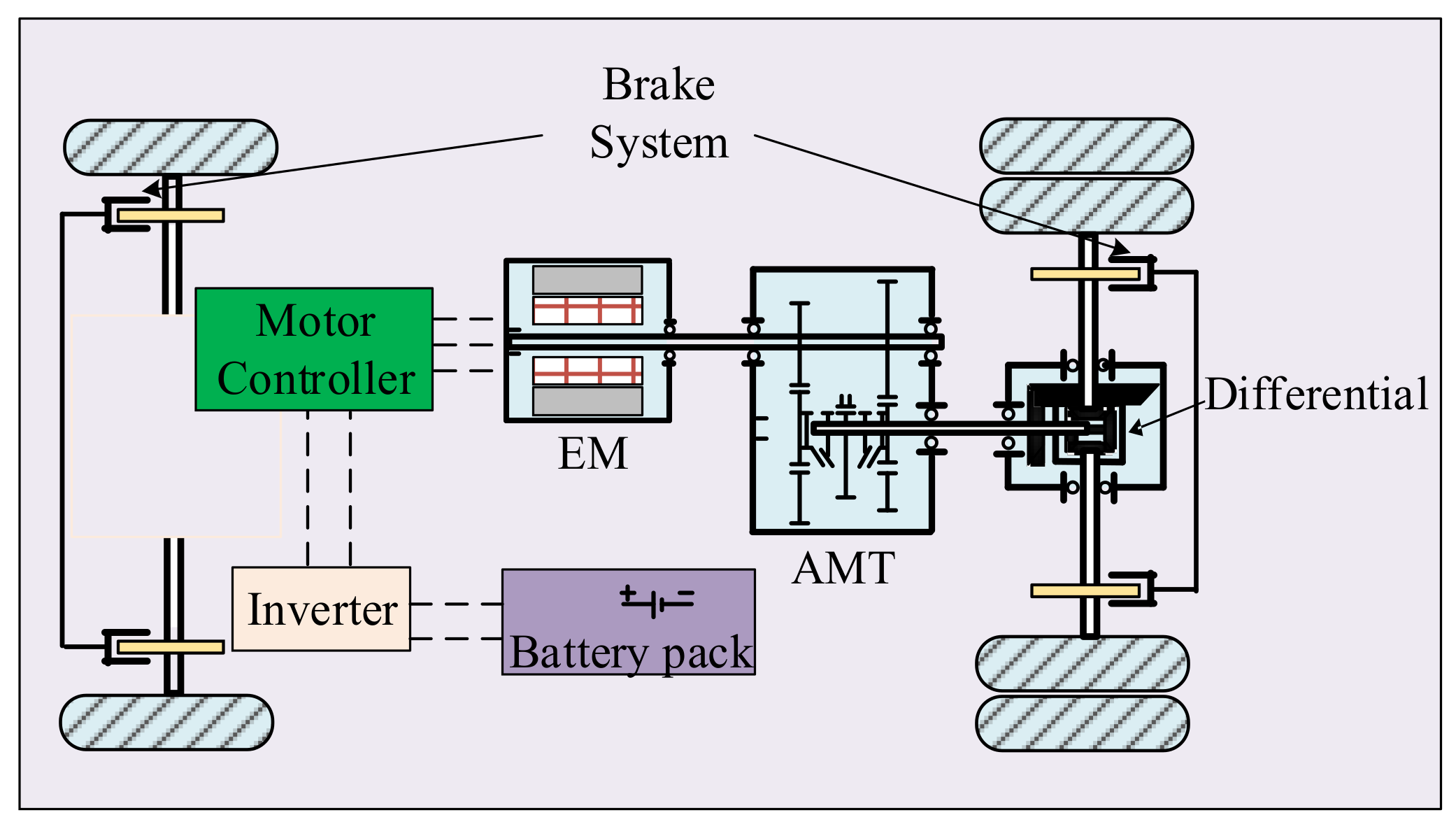
2. Model of Intelligent City Bus

A pure electric city bus is selected as the study platform in this paper. It is equipped with millimeter wave radar to detect position and speed information of preceding and current vehicles. The powertrain configuration of the bus is illustrated in Figure 1. It includes an electric motor (EM), a two-speed AMT, a differential, and the braking system. The EM is powered by a battery pack and is the only driving force provider in this system. When the vehicle brakes, EM can also provide braking force. The AMT can adjust output rotational speed by changing gear ratio [30]. The braking system refers to pneumatic electric braking system and it provides braking force when it receives braking command.

Key parameters of the city bus are shown in

Table 1. Key parameters of the city bus.

Parameters	Symbol	Value	Parameters	Symbol	Value
Bus Mass (kg)	$m$	-	time-delay constant of EM (s)	$\mathsf{\tau }$	0.5
Curb Mass (kg)	$m_{\min }$	12,200	output speed of EM (rpm)	$n_{EM}$	-
Gross Mass (kg)	$m_{\max }$	18,000	output speed of EM (rad/s)	${\omega }_{EM}$	-
Frontal Area (m2)	$A$	8.98	Final drive ratio	$i_0$	4.50
Air Resistance Coefficient	$C_D$	0.65	Gear ratio	$i_g$	[2.60, 1]
Road resistance coefficient	$f_r$	0.125	Transmission efficiency	${\eta }_{EM}$	0.85
Tire radius (m)	$r$	0.502	output power of battery (kW)	$P_{bat}$	-
rated/peak power of EM (kW)	$P_{EM}$	80/160	Voltage of Battery (V)	$U_{OC}$	-
rated/peak torque of EM (Nm)	$T_{EM}$	500/1100	internal resistance (Ω)	$R$	-
desired torque of EM (Nm)	$T_{EM}^{*}$	-	Capacity of Battery (A·h)	$Q_b$	348
regenerative torque of EM(Nm)	$T_{REG}$	-	State of Charge of Battery	$SoC$	-

. The gross mass is 12,200 kg, and when it is fully loaded with passengers, it reaches 18,000 kg. The bus is driving on the road with good road conditions, its rolling resistance coefficient is selected as 0.015.

2.1. EM Model

For EM, what we concern is the working efficiency. Therefore, its dynamic characteristics of output torque can be simplified as the first-order process [31]:

$$T_{EM}=\frac{T_{EM}^{*}}{1+\tau s}$$

(1)

where $T_{EM}$, $T_{EM}^{*}$, $\mathsf{\tau }$, and $s$ are output torque, desired torque, time-delay constant, and the frequency of the fist-order system. The energy utilization of the bus can be reflected by EM working efficiency and it is higher when the EM works at a relatively high efficiency. The energy consumption rate can be considered as a function of EM speed and EM torque, which can be expressed as follows:

$${\eta }_{EM}=f(n_{EM},T_{EM})$$

(2)

where ${\eta }_{EM}$ is the EM efficiency, it can be obtained from lookup table based on EM energy consumption MAP as shown in Figure 2. $n_{EM}$ is the rotational speed. When $T_{EM}$ is positive, the EM consumes electrical energy to drive the vehicle. When it is negative, the EM can be used as a generator to charge the battery if certain conditions are met.

2.2. Battery Model

For the battery pack, the relationships between open-circuit voltage, charging resistance, and state of charge (SoC) are complicated. In this paper, we don’t consider the effect of temperature and other factors, the relationships between them are shown in Figure 3.

The battery works safely and efficiently when SoC is between 0.5 and 0.75 and in this range, the value of internal resistance changes gently, so we can take it as a constant. For convenience, a simplified battery model with appropriate precision needs to be built, which simplify the battery as a voltage source with an internal resistance. Then, the gradient of SoC with time can be written as follows [32]:

$$\frac{\mathrm{d}SoC}{\mathrm{d}t}=-\frac{U_{OC}-\sqrt{U_{OC}^2-4R{P}_{ba}{}_t}}{2R{Q}_b}$$

(3)

where the $U_{OC}$, $R$, $Q_b$, and $P_{ba}{}_t$ are open-circuit voltage, internal resistance, the capacity of battery, and output power of battery.

When the bus drives, EM is a motor and it consumes battery energy. When the bus brakes, EM becomes a generator and it can provide energy for the battery by the regenerative braking system. Therefore, $P_{ba}{}_t$ can defined as follows:

$$P_{ba}{}_t=\left\{\begin{array}{ll}{T}_{EM}{\omega }_{EM}{\eta }_{EM}\hfill & {\omega }_{EM}\ge 0\hfill \\ \frac{T_{REG}{\omega }_{EM}}{{\eta }_{EM}}\hfill & {\omega }_{EM}<0\hfill \end{array}\right.$$

(4)

where ${\eta }_{EM}$, ${\omega }_{EM}$, and $T_{REG}$ are the efficiency of EM, the output speed of EM, and the regenerative torque of EM. In order to improve energy regenerative efficiency, the mechanical braking force of rear axle should be limited so that the EM should be involved in braking as much as possible. When EM cannot provide enough braking force, the mechanical brake then participates. For safety, the following restrictions are imposed on the regenerative braking force:

(1)

When SoC ≥ 0.8, for the safty of battery, EM is no longer engaged in braking and the mechanical braking system provides the brake torque. Thus, $T_{REG}$ = 0;

(2)

When the brake severity Z is in the range of 0 to 0.1, EM provides the brake torque for the vehicle and $T_{REG}$ = $T_{EM}$;

(3)

When Z is in the range of 0.1 to 0.7 or EM cannot provide enough brake torque, EM and mechanical braking system provides power for together. Thus, $T_{REG}$ = $T_{EM}$;

(4)

When Z > 0.7, EM quits from working and the braking power is provided by mechanical braking system. Thus, $T_{REG}$ = 0;

(5)

The EM braking effect is not obvious when its output speed below 500 r/min and the braking torque of the rear axle is provided by traditional mechanical braking system.

2.3. Vehicle Longitudinal Dynamics

When the bus is on a sloped road as shown in Figure 4, its longitudinal dynamic equation can be described as below:

$$m\dot{v}=F_t-F_{air}-F_{slope}-F_u$$

(5)

where $m$, $v$,$F_t$, $F_{air}$, $F_{slope}$, and $F_{\mu }$ are the bus mass, the longitudinal speed, the driving force acting on the wheels, the air resistance, the ramp resistance, and the rolling resistance, respectively. Therefore Equation (5) can be expanded as follows:

$$m\dot{v}=\frac{T_{EM}{i}_0{i}_g\eta }{r}-\frac{1}{2}{C}_{D}A\rho v^2-mg{f}_r\cos \theta -mg\sin \theta$$

(6)

where $i_0$ is the ratio of finial drive, $i_g$ is the ratio of AMT, $r$ is the wheel radius, $\eta$ is the transmission efficiency, $C_D$ is the air resistance coefficient, $A$ is the frontal area of the bus, $\rho$ is the air density (25 °C), $g$ is the acceleration of gravity, $f_r$ is rolling resistance coefficient, and $\theta$ is the road slope.

3. Problem Formulation

Two state space equations are described in this section: the state space equation for ACC and estimation equation for bus mass and road slope. Then the multi-objective optimization indexes are analyzed.

3.1. State Space Equation for ACC

The displacement, velocity, and SoC of the bus are defined as the state variables, so the state vector is $\mathit{x}={[s_{veh},v_{veh},SoC]}^T$. EM torque, braking torque, and gear position are selected as the control vector $\mathit{u}={[T_{EM},T_{Brk},i_g]}^T$. The road slope $\theta$ can be obtained by EFK, the distance between the two vehicles $s_{ref}-s_{veh}$, and the speed of the preceding vehicle $v_{veh}$ can be obtained by the radar. These external inputs are defined as $\mathit{d}={[\theta ,s_{ref}-s_{veh},v_{ref}]}^T$, where $s_{veh}$, $s_{ref}$,$v_{veh}$, and $v_{ref}$ are the traveling distance, speed of current vehicle, and preceding vehicle. The system states space equation can be written as follows:

$$\dot{\mathit{x}}=f(\mathit{x},\mathit{u},\mathit{d})$$

(7)

3.2. State Space for Vehicle Mass and Road Slope Estimating

Usually, the road slope cannot be obtained directly. In addition, the mass of the bus is not constant because of passengers constantly getting on and off. As important parameters of the vehicle longitudinal dynamic model, the vehicle mass and road slope should be determined. The EKF algorithm is used to estimate the two variables in this section.

The state variables are defined as $\mathit{x}={[v,m,\theta ]}^T$. Considering the nonlinear relationship between the road slope and vehicle mass, the road slope can be regarded as zero in a relatively short time interval. Combining with Equation (1), the differential equations can be given as:

$$\left\{\begin{array}{l}\dot{v}(t)=\frac{T_{EM}(t)i_0{i}_g}{m(t)r}-gf-\frac{1}{2m(t)}{C}_{D}A\rho v^2(t)-g\theta (t)\hfill \\ \dot{m}(t)=0\hfill \\ \dot{\theta }(t)=0\hfill \end{array}\right.$$

(8)

The EKF algorithm is based on discrete state space equation, and the forward Euler method is used to the discrete Equation (8). It can be obtained as follows:

$$\left\{\begin{array}{l}{v}_k=v_{k-1}+\Delta t\left(\frac{T_{EM}(t_{k-1})i_0{i}_g\eta }{m_{k-1}r}-gf-\frac{1}{2m_{k-1}}{C}_{D}A\rho v_{k-1}^2-g{\theta }_{k-1}\right)\hfill \\ m_k=m_{k-1}\hfill \\ {\theta }_k={\theta }_{k-1}\hfill \end{array}\right.$$

(9)

Therefore, the state of the system can be written as follows:

$$\left[\begin{array}{c}{v}_k\\ m_k\\ {\theta }_k\end{array}\right]=\left[\begin{array}{c}{v}_{k-1}+(\dot{v}(t_{k-1}))\Delta t\\ m_{k-1}\\ {\theta }_{k-1}\end{array}\right]+{\mathit{W}}_{k-1}$$

(10)

where:

$$\dot{v}(t_{k-1})=\frac{T_{EM}(t_{k-1})i_g{i}_0\eta }{m_{k-1}r}-gf-\frac{1}{2m_{k-1}}{C}_{D}A\rho v_{k-1}^2-g{\theta }_{k-1}$$

(11)

The observed equation can be written as:

$$z_k=[\begin{array}{ccc}1& 0& 0\end{array}]\left[\begin{array}{c}{v}_k\\ m_k\\ {\theta }_k\end{array}\right]+{\mathit{V}}_k$$

(12)

Combining with Equation (10), the state space can be expressed as follows:

$$\left\{\begin{array}{c}x=f(x_{k-1})+{\mathit{W}}_{k-1}\\ z_k=\mathit{H}{x}_k+{\mathit{V}}_k\end{array}\right.$$

(13)

where $\mathit{H}=[\begin{array}{ccc}1& 0& 0\end{array}]$ is the measuring matrix $\mathit{W}$ and $\mathit{V}$ are noise vector, which are independent white Gaussian noise with zero mean. The EKF algorithm that employed to estimate the vehicle mass and road slope includes two processes: the time update and the measuring update. The equations of updating time can be described as follows:

$$\left\{\begin{array}{l}{\hat{x}}_k^{-}=f({\hat{x}}_{k-1}^{-})\hfill \\ {\mathit{P}}_k^{-}=\mathit{A}(k){\mathit{P}}_{k-1}\mathit{A}{(k)}^T+{\mathit{Q}}_{k-1}\hfill \end{array}\right.$$

(14)

where ${\hat{x}}_k^{-}$, ${\hat{x}}_{k-1}^{-}$, ${\mathit{P}}_k^{-}$, ${\mathit{P}}_{k-1}$, and ${\mathit{Q}}_{k-1}$ are the optimal prediction of observer estimation, the optimal estimation of state variables of last step, error covariance matrix estimated from the last matrix, the error covariance matrix of last step, and covariance matrix of noise process, respectively. $\mathit{A}(k)$ is the state transition matrix and it is the Jacobian matrix obtained as follows:

$$\mathit{A}(k)=\frac{\partial f(\hat{x}(k))}{dx}=\left[\begin{array}{ccc}{\mathit{A}}_1& {\mathit{A}}_2& {\mathit{A}}_3\\ 0& 1& 0\\ 0& 0& 1\end{array}\right],$$

(15)

where ${\mathit{A}}_1$, ${\mathit{A}}_2$, ${\mathit{A}}_3$ can be described as follows:

$$\left\{\begin{array}{l}{\mathit{A}}_1=1-\frac{C_{D}A\rho v}{m}\Delta t\hfill \\ {\mathit{A}}_2=\frac{C_{D}A\rho v^{2}r-2T_{EM}{i}_g{i}_0\eta }{2m^{2}r}\hfill \\ {\mathit{A}}_3=-g\Delta t\hfill \end{array}\right..$$

(16)

The measuring updating equation is defined as follows:

$$\left\{\begin{array}{c}{\mathit{K}}_k={\mathit{P}}_k^{-}{\mathit{H}}^T{(\mathit{H}{\mathit{P}}_k^{-}{H}^T+{\mathit{R}}_k)}^{-1}\\ {\mathit{P}}_k=(\mathbf{I}-{\mathit{K}}_k\mathit{H}){\mathit{P}}_k^{-}\\ {\widehat{x}}_k={\widehat{x}}_k^{-}+{\mathit{K}}_k(z_k-\mathit{H}{\widehat{x}}_k^{-})\end{array}\right.$$

(17)

where ${\mathit{K}}_k$, ${\mathit{P}}_k$, $\mathit{I}$, and ${\hat{x}}_k$ are gains of Kalman filter, error covariance of observer estimation, the unit matrix, and the optimal estimation of observed elements respectively.

3.3. ACC Optimizing Indexes

As one important component of ACC, the spacing strategy determines the safe following distance and provides the reference input values for the subsequent control algorithm. These indexes that should be optimized are the following distance$\Delta s$, the relative speed $\Delta v$, the relative acceleration $\Delta a$, and the vehicle jerk $j_{veh}={\mathrm{da}}_{veh}/\mathrm{d}t$. They are described in the following text.

Safety is the primary requirement in ACC. To avoid collision between the current and preceding vehicle, the minimum following distance should be longer than the braking distance. The braking distance can be obtained as [33]:

$$s_{Brk}=v_{veh}{\mathsf{\tau }}_{Brk}+\frac{v_{veh}^2}{2a_{Brk}}$$

(18)

where ${\mathsf{\tau }}_{Brk}$ is the reaction time of braking system, we assume it is 0.5 s. $a_{Brk}$ is the braking deceleration; the maximum braking deceleration is 8 m/s². This paper assumes that after the emergency braking, the final minimum and maximum distance between the two vehicles is 2m and 8m. Therefore, Equation (18) can be expended as follows [34]:

$$\left\{\begin{array}{c}\Delta s_{\min }=2+0.5\cdot v_{veh}+0.0625\cdot v_{veh}^2\\ \Delta s_{\max }=8+0.5\cdot v_{veh}+0.0625\cdot v_{veh}^2\end{array}\right.$$

(19)

where $\Delta s_{\min }$ and $\Delta s_{\max }$ are the minimum and maximum safety following distance. We can define the optimal braking distance with the adjustment coefficient $\alpha$:

$$\left\{\begin{array}{c}\Delta s_{up}=\alpha \cdot \Delta s_{\max }+(1-\alpha )\cdot \Delta s_{\min }\\ \Delta s_{low}=\alpha \cdot \Delta s_{\min }+(1-\alpha )\cdot \Delta s_{\max }\end{array}\right.$$

(20)

where $\Delta s_{up}$ and $\Delta s_{low}$ are the upper and lower bound of the optimal distance zone. The relationship between the following distance and the longitudinal speed of the vehicle is shown in Figure 5.

The relevant traveling distance $\Delta s$ should be restricted in the optimal distance area, when it is out of the area, there will be a cost coefficient. When $\Delta s$ is larger than $\Delta s_{up}$, the cost coefficient will be very large. When $\Delta s$ is smaller than $\Delta s_{low}$, it means the preceding vehicle and the current vehicle may collide and this situation is not allowed. Therefore, the cost function of $\Delta s$ can be defined as:

$$J_{\Delta s}=\left\{\begin{array}{ll}+\infty ,\hfill & \Delta s<\Delta s_{\min }\hfill \\ k_1\cdot \tan (\frac{\Delta s-\Delta s_{low}}{\Delta s_{\min }-\Delta s_{low}}\cdot \frac{\pi }{2}),\hfill & \Delta s_{\min }\le \Delta s<\Delta s_{low}\hfill \\ \left|\Delta s-\frac{\Delta s_{up}+\Delta s_{low}}{2}\right|,\hfill & \Delta s_{low}\le \Delta s<\Delta s_{up}\hfill \\ k_2\cdot {(\Delta s-\Delta s_{up})}^2,\hfill & \Delta s_{up}\le \Delta s<\Delta s_{\max }\hfill \\ k_3\cdot {(\Delta s-\Delta s_{\max })}^2+k_2\cdot {(\Delta s-\Delta s_{up})}^2,\hfill & \Delta s>\Delta s_{\max }\hfill \end{array}\right.$$

(21)

where $k_1$, $k_2$, and $k_3$ are the cost coefficients. As for the cost function about longitudinal speed and acceleration, we define them by $\Delta v$ and $\Delta a$:

$$\left\{\begin{array}{c}{J}_{\Delta v}=k_4\cdot \Delta v^2\\ J_{\Delta a}=k_5\cdot \Delta a^2\end{array}\right.$$

(22)

where $k_4$ and $k_5$ are the cost coefficients. The cost function corresponding to the vehicle jerk (the time rate of change of acceleration) has great effect on ride comfort:

$$J_{jerk}=\left\{\begin{array}{cc}{k}_6\cdot j_{veh}^2& \left|j_{veh}\right|>3 m/s^2\\ 0& \left|j_{veh}\right|\le 3 m/s^2\end{array}\right.,$$

(23)

where $k_6$ is the cost coefficient. When $j_{veh}\le 3$, we think the jerk is small and the vehicle movies smoothly, so $J_{jerk}=0$.

In order to optimize energy consumption, economic optimizing indexes should be defined. Considering that EM power represents the consumption of electrical energy. The cost function of economic optimizing index can be defined as:

$$J_{eco}={\displaystyle {\int }_0^{t_f}(T_{EM}\cdot {\omega }_{EM}\cdot {\eta }_{EM}})dt.$$

(24)

In summary, the cost function of optimizing indexes can be expressed as follows:

$$J_{opt}={\displaystyle {\int }_0^{t_f}(J_{\Delta s}+J_{\Delta v}+J_{\Delta a})dt}+J_{eco}$$

(25)

In Equation (24), $t_f$ is the period of MPC predictive horizon described in Section 3.4. From Equations (21)–(24), we get the cost coefficients of following distance, relevant speed, relevant acceleration, and jerk at a certain moment. Therefore, the integrated indexes ${\displaystyle {\int }_0^{t_f}{J}_{\Delta s}dt}$, ${\displaystyle {\int }_0^{t_f}{J}_{\Delta v}dt}$, ${\displaystyle {\int }_0^{t_f}{J}_{\Delta a}dt}$, and ${\displaystyle {\int }_0^{t_f}{J}_{jerk}dt}$ are the total cost coefficient in the MPC predictive horizon. In the ACC process, the following distance is the most important for safety, followed by the comfort of passengers, and then consider energy saving on this basis. Therefore, $k_1$, $k_2$, and $k_3$ related to the following distance have the highest priority, followed by them are the comfort-related factors $k_4$, $k_5$, and finally $k_6$ is adjusted to make the vehicle have better energy saving performance.

3.4. MPC Optimizing Algorithm

The nonlinear MPC algorithm is proposed to optimize the tracking capability, driving safety, driving comfort, and energy consumption. In Section 3.1, the state vector has been known and coordinating with the vehicle dynamics model, the discretization of system predictive model can be written as follows:

$$s_{veh}(k+1)=s_{veh}(k)+v_{veh}\cdot T_s+\frac{1}{2}{a}_{veh}(k)\cdot T_s^2$$

(26)

$$v_{veh}(k+1)=v_{veh}(k)+a_{veh}(k)\cdot T_s$$

(27)

$$SoC(k+1)=SoC(k)-\frac{U_{oc}-\sqrt{U_{oc}^2-4R{T}_m(k){{\omega }}_m(k){{\eta }}_m^a(k)}}{2R{Q}_b}\cdot T_s$$

(28)

Therefore, Equation (7) can be expressed as follows:

$$\mathit{x}(k+1)=f(\mathit{x}(k),\mathit{u}(k),\mathit{d}(k)).$$

(29)

Considering the nonlinearity of the system, it is hard to know the analytical solution by receding horizon optimization. In this paper, the optimal solution of the system can be obtained by enumerating the control vectors: Firstly, enumerating the $a_{veh}$ which is restricted from $a_{\min }$ to $a_{\max }$ and the optimization indexes can be calculated. Then, it can be determined if the loop should continue by judging whether the indexes are the most optimal indexes.

In this paper, the sample time is set as 0.1 s, predictive horizon $P$ equals 8 to avoid the whole prediction time exceeds 1 s, and the control horizon is set as 1. In the ACC process, the bus mass and road slope are changing with time and the EFK method is used to estimate the two variables. The MPC + EKF combining algorithm is described in Figure 6.

4. Simulation and Experiment Results

In this section, the simulations are implemented in MATLAB/Simulation to show the performance of the proposed control strategy. Then the HIL test is carried out to vary the simulation results.

4.1. Driving Cycles

The driving cycle mainly refers to these aspects: (1) the speed curve of the preceding vehicle; (2) the road slope and the position of bus stations; (3) the mass curve of the current bus.

In ACC process, the speed of the preceding vehicle can be obtained by millimetre-wave radars, which is shown in Figure 7. It can be seen that the driving cycle lasts 1220 s and the maximum speed is 50 km/h. Figure 8 is the changes of bus mass and road slope. At the first station, the vehicle mass increased from 14 to 18 tons. At the second station, it decreased from 18 to 12 tons. The road slope changes throughout the whole ACC process and its range are varied from −8 to +8%.

The value of cost coefficients should be determined to adjust the magnitudes of $J_{\Delta s}$,$J_{\Delta v}$, $J_{\Delta a}$ and $J_{jerk}$ at the same order magnitude. For example, the valve of $\Delta v^2$ and $\Delta a^2$ are 10² and 10¹ in most conditions, so the magnitude of $k_4$ and $k_5$ are chosen as 50 and 100 to balance the proportion of $J_{\Delta s}$ and $J_{\Delta v}$. The key simulation parameters involved in this paper are listed in

Table 2. Simulation parameters.

Parameters	Symbol	Value
Predictive horizon	P	8
Control horizon	m	1
Optimal distance efficient	α	0.4
Distance cost efficient Ⅰ	k1	200
Distance cost efficient Ⅱ	k2	100
Distance cost efficient Ⅲ	k3	1000
Speed cost efficient	k4	50
Acceleration cost efficient	k5	100
Jerk cost efficient	k6	10

.

4.2. Simulation Results

In this section, the simulation results of proposed strategy MPC + EKF are analyzed as follows.

The simulation results of the longitudinal speed are shown in Figure 9. It can be seen that there are several sudden changes of the preceding vehicle speed and the current vehicle controlled by MPC + EKF strategy follows the preceding bus very well. From Figure 5, we know the following distance is related to the vehicle speed, so the shape of the following distance shown in Figure 10 is coincidentally similar to the vehicle speed. It can be seen that throughout the ACC process, the actual following distance is always between the maximum and minimum safe following distances. It means the proposed MPC + EKF strategy can guarantee the tracking ability and driving safety of ACC.

As a comparison, the speed of the current vehicle without the EKF strategy is also shown in Figure 9. It can be clearly divided into three zones. At the first zone, the estimated speed without EKF can follow the preceding vehicle but not well because the road slope has changed and the mass has not changed. At the second zone, the estimating speed without EKF is far below the preceding vehicle speed, because the vehicle mass has increased to 18 tons while the mass in the vehicle dynamics model is still 14 tons (the mass is not estimated and it is a constant), so the EM torque is not enough to increase the speed to the preceding vehicle’s speed. At the third zone, the vehicle mass has reduced to 12 tons, opposite to the second zone, the EM torque is too large, causing the vehicle speed to overtake the preceding vehicle severely. Therefore, without the estimation for vehicle mass and road slope, the tracking ability and driving safety in ACC is hard to achieve.

As shown in Figure 11, The traveling distance of preceding and current vehicles is about 8.1 km. During the ACC process, the actual traveling distance of the current bus is always smaller than the preceding one. The distance between the two buses is shown in Figure 12, it can be seen that the distance is almost within the safety zone. That is, the following distance meets the safety demand.

Figure 13a,b are the jerk of the two vehicles. Obviously, the jerk of current vehicle mainly fluctuates in the range of ±5 m/s³ and it is smaller than that of the preceding vehicle in the range of ±40 m/s³. Therefore, the ride comfort of the current vehicle is better than the preceding vehicle.

The reduction of battery SoC means energy consumption, meanwhile, as described in Section 2.2, when EM works as a generate. Therefore, we measure vehicle energy efficiency by how much SoC is reduced. In this paper, the parameters of the preceding vehicle are the same as those of the current vehicle. Figure 14 shows the change of SoC by time during ACC process. It can be seen that the SoC of the preceding vehicle reduced from 65 to 61% and that of the current vehicle reduced from 65 to 62%. The current vehicle saved about 10% energy compared to the preceding vehicle in per 100 km. This is because when under the control of MPC + EKF strategy, the jerk of current bus results in smaller changes than that of the preceding bus.

Figure 15 and Figure 16 show the results of vehicle mass estimation and road slope estimation obtained by EKF. The estimated results have errors with the real values, but the trends are the same. In Figure 15, the initial estimated mass is far from the actual value and after about 20 s, the estimated mass gradually approaches the true value. As the city bus arrives at the first station, its mass increases to 18 tons, the estimated value is close to the real value after 25 s. The situation of the second station is as the same as the first station.

Figure 17 shows the error of the mass estimation. It can be seen that the error is changing at the range of −5 to +5%. When the vehicle mass changes, the mass error of estimation can be reduced to within 5% in 38 s. Figure 16 is the result of road slope estimation. We can know that there are some slight shakes of the estimated value, but it is basically consistent with the actual slope. Usually, an error of no more than 5% is the requirement of the vehicle mass estimation. Compared with the vehicle mass estimation on the fixed road slope, the strategy adopted in this paper can achieve the same accuracy for the vehicle mass estimation on a changing road slope, and the shaking is smaller [35].

4.3. Experiment Test Bases on HIL

The HIL simulation is illustrated in Figure 18 and it adopts the hierarchical control strategy. The upper level mainly includes the Real-Time System (RTS) which can guarantee the real-time performance of HIL simulation. The Host PC can download the proposed control strategy programs to ECU, and the vehicle dynamic model runs in PXI. The lower level mainly means the braking system and the driving system, as shown in Figure 19, they can implement driving and braking functions when receiving the signals from the upper level by CAN communication. In the braking system, the proportional valve and the relay valve can adjust the brake pressure according to the received desired brake signal. Similarly, the desired torque signal is transported to EM controller to adjust the driving force.

During the driving cycle, when the pneumatic braking system works, the proportional valve starts to pressurize the brake chamber to achieve the braking and the pressure can be acquired by pressure sensor.

The driving cycle of the HIL test is the same as the simulation. Figure 20 is the vehicle longitudinal velocity test result from 535 s to 720 s. It can be seen that the estimated velocity with EKF control strategy follows the desired velocity well. In contrast to this, the velocity result without EKF control strategy has obvious errors with the desired velocity. This is because the bus is running in the second zone, as described in Figure 10, and the real vehicle mass is 18 tons while the mass in the control strategy without EKF is 14 tons and the large mass error making the inaccurate results. Therefore, the HIL test results are agree with the simulation results.

Figure 21 shows the change of braking force at 535 s to 720 s of the whole ACC process. The desired force comes from the output of MPC+EKF strategy. The actual force is obtained from the force sensor of the HIL test bench. It can be seen that the actual force has some shake when the desired force is zero, but when braking occurs, the actual braking force follows the desired well. Figure 22 shows the change of braking pressure in the same time period. Similar to braking force, the desired pressure comes from simulation and the actual pressure comes from the pressure sensor. It can be seen that the actual pressure has a certain delay to the desired one due to mechanical delays. Overall, the simulated pressure can reflect the actual brake pressure.

The adjustment result of EM torque is shown in Figure 23. Similarly to the pressure control, the desired EM torque is calculated from the control strategy and the actual torque is obtained from the EM in the HIL test bench. We can see the actual torque follows the desired torque well and there is a certain delay between the desired torque and the actual torque as described in Section 2.1.

The HIL test results show that the tracking ability and the braking capacity can be guaranteed during the ACC process. The proposed EKF + MPC control strategy can work in the actual condition.

5. Conclusions

This paper takes intelligent city bus as the platform and uses the EKF strategy to estimate the vehicle mass and the road slope. Then, combining the MPC strategy to design a multi-objective optimized control strategy to balance vehicle tracking ability, driving safety, driving comfort, and energy saving. The MATLAB/Simulink simulation and HIL experiments were carried to implement and verify the control strategy. The conclusions are as follows:

(1)

The EKF strategy was used to realize the real-time estimation of vehicle mass and road slope. The estimation error of vehicle mass can be reduced to within ±5% in 40 s, and the estimation error of road slope can follow the actual value well. Real-time estimation for mass and slope provides key parameters for ACC implementation;

(2)

In this paper, we established the cost functions about speed, acceleration, impact, and SoC. Based on cost functions, we proposed the nonlinear MPC control algorithm. By adjusting the cost coefficients, we realized the multi-objective optimization of ACC;

(3)

Through simulation and HIL experiments, the feasibility of the EKF+MPC control strategy was verified. On the basis of ensuring safety and tracking ability, the maximum impact of the current vehicle was reduced to 5 m/s³, the consumption of the SoC was reduced by about 10%, and the vehicle comfort and energy efficiency are well improved.

References

1. Lv, C.; Xing, Y.; Zhang, J.; Na, X.; Li, Y.; Liu, T.; Cao, D.; Wang, F.-Y. Levenberg–Marquardt Backpropagation Training of Multilayer Neural Networks for State Estimation of a Safety-Critical Cyber-Physical System. IEEE Trans. Ind. Inform. 2018, 14, 3436–3446. [Google Scholar] [CrossRef] [Green Version]
2. Yang, C.; You, S.; Wang, W.; Li, L.; Xiang, C. A stochastic predictive energy management strategy for plug-in hybrid electric vehicles based on fast rolling optimization. IEEE Trans. Ind. Electron. 2019, 67, 9659–9670. [Google Scholar] [CrossRef]
3. Sun, Y.; Wang, X.; Li, L.; Shi, J.; An, Q. Modelling and control for economy-oriented car-following problem of hybrid electric vehicle. IET Intell. Transp. Syst. 2019, 13, 825–833. [Google Scholar] [CrossRef]
4. Zhang, Y.; Shen, X.; Raksincharoensak, P. Automated Vehicle’s Overtaking Maneuver with Yielding to Oncoming Vehicles in Urban Area Based on Model Predictive Control. Appl. Sci. 2021, 11, 9003. [Google Scholar] [CrossRef]
5. Chen, J.; Zhou, Y.; Liang, H. Effects of ACC and CACC vehicles on traffic flow based on an improved variable time headway spacing strategy. IET Intell. Transp. Syst. 2019, 13, 1365–1373. [Google Scholar] [CrossRef]
6. Guo, C.; Meguro, J.; Kojima, Y.; Naito, T. A multimodal ADAS system for unmarked urban scenarios based on road context understanding. IEEE Trans. Intell. Transp. Syst. 2015, 16, 1690–1704. [Google Scholar] [CrossRef]
7. Schreier, M.; Willert, V.; Adamy, J. Compact representation of dynamic driving environments for ADAS by parametric free space and dynamic object maps. IEEE Trans. Intell. Transp. Syst. 2016, 17, 367–384. [Google Scholar] [CrossRef]
8. Cheng, S.; Li, L.; Mei, M.M.; Nie, Y.L.; Zhao, L. Multiple objective adaptive cruise control system integrated with DYC. IEEE Trans. Veh. Technol. 2019, 68, 4550–4559. [Google Scholar] [CrossRef]
9. Kim, H.; Kim, D.; Shu, I.; Yi, K. Time-varying parameter adaptive vehicle speed control. IEEE Trans. Veh. Technol. 2015, 65, 581–588. [Google Scholar] [CrossRef]
10. Ren, Y.; Zheng, L.; Yang, W.; Li, Y. Potential field–based hierarchical adaptive cruise control for semi-autonomous electric vehicle. Proc. Inst. Mech. Eng. Part. D J. Automob. Eng. 2019, 233, 2479–2491. [Google Scholar] [CrossRef]
11. Zhang, J.; Ioannou, P.A. Longitudinal control of heavy trucks in mixed traffic: Environmental and fuel economy considerations. IEEE Trans. Intell. Transp. Syst. 2006, 7, 92–104. [Google Scholar] [CrossRef]
12. Ganji, B.; Kouzani, A.Z.; Khoo, S.Y.; Shams-Zahraei, M. Adaptive cruise control of a HEV using sliding mode control. Expert Syst. Appl. 2014, 41, 607–615. [Google Scholar] [CrossRef]
13. Shakouri, P.; Ordys, A.; Askari, M.R. Adaptive cruise control with stop & go function using the state-dependent nonlinear model predictive control approach. ISA Trans. 2012, 51, 622–631. [Google Scholar]
14. Luo, Y.; Chen, T.; Li, K. Multi-objective decoupling algorithm for active distance control of intelligent hybrid electric vehicle. Mech. Syst. Signal. Process. 2015, 64, 29–45. [Google Scholar] [CrossRef]
15. Luo, Y.; Chen, T.; Zhang, S.; Li, K. Intelligent hybrid electric vehicle ACC with coordinated control of tracking ability, fuel economy, and ride comfort. IEEE Trans. Intell. Transp. Syst. 2015, 16, 2303–2308. [Google Scholar] [CrossRef]
16. Mantovani, G.; Ferrarini, L. Temperature control of a commercial building with model predictive control techniques. IEEE Trans. Ind. Electron. 2014, 62, 2651–2660. [Google Scholar] [CrossRef]
17. Choi, D.K.; Lee, K. Dynamic performance improvement of AC/DC converter using model predictive direct power control with finite control set. IEEE Trans. Ind. Electron. 2014, 62, 757–767. [Google Scholar] [CrossRef]
18. Sun, J.; Ghaemi, R.; Kolmanovsky, I.; Tao, G. Developments in receding horizon optimization-based controls: Towards real-time implementation for nonlinear systems with fast dynamics. In Advances in Control Theory and Applications; Springer: Berlin, Germany, 2008. [Google Scholar]
19. Li, S.E.; Jia, Z.; Li, K.; Cheng, B. Fast online computation of a model predictive controller and its application to fuel economy–oriented adaptive cruise control. IEEE Trans. Intell. Transp. Syst. 2014, 16, 1199–1209. [Google Scholar] [CrossRef]
20. Cagienard, R.; Grieder, P.; Kerrigan, E.; Morari, M. Move blocking strategies in receding horizon control. J. Process. Control. 2007, 17, 563–570. [Google Scholar] [CrossRef] [Green Version]
21. Li, L.; Jia, G.; Chen, J.; Zhu, H.; Cao, D.; Song, J. A novel vehicle dynamics stability control algorithm based on the hierarchical strategy with constrain of nonlinear tyre forces. Veh. Syst. Dyn. 2015, 53, 1093–1116. [Google Scholar] [CrossRef]
22. Li, S.E.; Li, K.; Wang, J. Economy-oriented vehicle adaptive cruise control with coordinating multiple objectives function. Veh. Syst. Dyn. 2013, 51, 1–17. [Google Scholar]
23. Marzbanrad, J.; Karimian, N. Space control law design in adaptive cruise control vehicles using model predictive control. Proc. Inst. Mech. Eng. Part. D J. Automob. Eng. 2011, 225, 870–884. [Google Scholar] [CrossRef]
24. Zhang, X.; Xu, L.; Li, J.; Ouyang, M. Real-Time estimation of vehicle mass and road slope based on multi-sensor data fusion. In Proceedings of the IEEE Vehicle Power and Propulsion Conference (VPPC), Beijing. China, 15–18 October 2013. [Google Scholar]
25. Kim, D.; Choi, S.B.; Choi, M. Integrated vehicle mass estimation for vehicle safety control using the recursive least-squares method and adaptation laws. Proc. Inst. Mech. Eng. Part. D J. Automob. Eng. 2015, 229, 14–24. [Google Scholar] [CrossRef]
26. Vahidi, A.; Stefanopoulou, A.; Peng, H. Recursive least squares with forgetting for online estimation of vehicle mass and road slope: Theory and experiments. Veh. Syst. Dyn. 2005, 43, 31–55. [Google Scholar] [CrossRef]
27. Ding, F.; Wang, Y.; Ding, J. Recursive least squares Parameter identification algorithms for systems with colored noise using the filtering technique and the auxiliary model. Digit. Signal. Process. 2015, 37, 100–108. [Google Scholar] [CrossRef]
28. Raffone, E. Road slope and vehicle mass estimation for light commercial vehicle using linear Kalman filter and RLS with forgetting factor integrated approach. In Proceedings of the 16th International Conference on Information Fusion, Istanbul, Turkey, 9–12 July 2013. [Google Scholar]
29. Korayem, A.H.; Khajepour, A.; Fidan, B. Trailer mass estimation using system model-based and machine learning approaches. IEEE Trans. Veh. Technol. 2020, 69, 12536–12546. [Google Scholar] [CrossRef]
30. Zhu, X.; Zhang, H.; Feng, Z. Speed synchronization control for integrated automotive motor-transmission powertrain system with random delays. Mech. Syst. Signal. Process. 2015, 64/65, 46–57. [Google Scholar] [CrossRef]
31. Li, L.; You, S.; Yang, C.; Yan, B.; Song, J.; Chen, Z. Driving-behavior-aware stochastic model predictive control for plug-in hybrid electric buses. Appl. Energy 2016, 162, 868–897. [Google Scholar] [CrossRef]
32. Liu, B.; Li, L.; Wang, X.; Cheng, S. Hybrid electric vehicle downshifting strategy based on stochastic dynamic programming during regenerative braking process. IEEE Trans. Veh. Technol. 2018, 67, 4716–4727. [Google Scholar] [CrossRef]
33. Wang, X.; Li, L.; Yang, C. Hierarchical control of dry clutch for engine-start process in a parallel hybrid electric vehicle. IEEE Trans. Transp. Electrif. 2016, 2, 231–243. [Google Scholar] [CrossRef]
34. Li, L.; Wang, X.; Song, J. Fuel consumption optimization for smart hybrid electric vehicle during a car-following process. Mech. Syst. Signal. Process. 2017, 87, 17–29. [Google Scholar] [CrossRef]
35. Peng, P.; Wang, H.; Pi, D.; Wang, E.; Yin, G. Two-layer mass-adaptive hill start assist control method for commercial vehicles. Proc. Inst. Mech. Eng. Part. D J. Automob. Eng. 2020, 234, 438–448. [Google Scholar] [CrossRef]
Figure 1. Schematic graph of PEB powertrain structure.
Applsci 11 12137 g001
Figure 2. The MAP chart for EM efficiency.
Applsci 11 12137 g002
Figure 3. The battery parameters.
Applsci 11 12137 g003
Figure 4. The schematic diagram when the bus is running on ramp.
Applsci 11 12137 g004
Figure 5. The relationship between the following distance and longitudinal speed.
Applsci 11 12137 g005
Figure 6. The flow chats of MPC+EKF control strategy.
Applsci 11 12137 g006
Figure 7. The longitudinal speed of the preceding vehicle.
Applsci 11 12137 g007
Figure 8. The changes of vehicle mess and road slope.
Applsci 11 12137 g008
Figure 9. The simulation results of the longitudinal speed.
Applsci 11 12137 g009
Figure 10. The following distance of preceding vehicle and current vehicle.
Applsci 11 12137 g010
Figure 11. The traveling distance of preceding vehicle and current vehicle.
Applsci 11 12137 g011
Figure 12. The traveling distance between preceding vehicle and current vehicle.
Applsci 11 12137 g012
Figure 13. (a) The jerk of the preceding vehicle; (b) The jerk of the current vehicle.
Applsci 11 12137 g013
Figure 14. The SoC change of preceding vehicle and current vehicle.
Applsci 11 12137 g014
Figure 15. The estimation of vehicle mass.
Applsci 11 12137 g015
Figure 16. The result of road slope estimation.
Applsci 11 12137 g016
Figure 17. The error of the mass estimation.
Applsci 11 12137 g017
Figure 18. The structure of HIL test bench.
Applsci 11 12137 g018
Figure 19. Photo of the HIL test bench.
Applsci 11 12137 g019
Figure 20. The result of vehicle velocity.
Applsci 11 12137 g020
Figure 21. The adjustment results of braking torque.
Applsci 11 12137 g021
Figure 22. The adjustment results of braking pressure.
Applsci 11 12137 g022
Figure 23. The adjustment results of driving torque.
Applsci 11 12137 g023