Article

Rail Diagnostics Based on Ultrasonic Guided Waves: An Overview

by
Davide Bombarda
1,*,
Giorgio Matteo Vitetta
1 and
Giovanni Ferrante
2
1
Department of Engineering “Enzo Ferrari”, University of Modena and Reggio Emilia, 41125 Modena, Italy
2
Alstom Ferroviaria S.p.A., 40128 Bologna, Italy
*
Author to whom correspondence should be addressed.
Appl. Sci. 2021, 11(3), 1071; https://doi.org/10.3390/app11031071
Submission received: 18 December 2020 / Revised: 18 January 2021 / Accepted: 19 January 2021 / Published: 25 January 2021
(This article belongs to the Special Issue Novel Approaches for Structural Health Monitoring)

Abstract

:
Rail tracks undergo massive stresses that can affect their structural integrity and produce rail breakage. The last phenomenon represents a serious concern for railway management authorities, since it may cause derailments and, consequently, losses of rolling stock material and lives. Therefore, the activities of track maintenance and inspection are of paramount importance. In recent years, the use of various technologies for monitoring rails and the detection of their defects has been investigated; however, despite the important progresses in this field, substantial research efforts are still required to achieve higher scanning speeds and improve the reliability of diagnostic procedures. It is expected that, in the near future, an important role in track maintenance and inspection will be played by the ultrasonic guided wave technology. In this manuscript, its use in rail track monitoring is investigated in detail; moreover, both of the main strategies investigated in the technical literature are taken into consideration. The first strategy consists of the installation of the monitoring instrumentation on board a moving test vehicle that scans the track below while running. The second strategy, instead, is based on distributing the instrumentation throughout the entire rail network, so that continuous monitoring in quasi-real-time can be obtained. In our analysis of the proposed solutions, the prototypes and the employed methods are described.

1. Introduction

The track is one of the basic elements of railroading. Since the weight of trains is discharged on a very small portion of rail surfaces, tracks require careful maintenance [1]. It is well known that: (a) rails are subject to intense bending and shear stresses, plastic deformation and wear, leading to progressive degradation of their structural integrity [2]; (b) they may contain internal fabrication defects undetected by quality control. All of this may result in rail breakage and, consequently, in train derailment with potential catastrophic consequences (traffic interruption, possible losses of rolling stock material and even lives, etc.).
According to the European Union agency for railways (ERA) safety overview for 2017 [3], in the years 2011–2015, broken rails have represented the main form of precursors to accidents, i.e., of inconveniences that, under other circumstances, could have led to an accident (other precursors to accidents include track buckles, signals passed at danger, wrong-side signaling failures, broken wheels, and axles). On the average, 4445 broken rails per year have been detected over a total of 11,222 precursors to accidents in the whole European Union (EU-28) in the same period. This explains why track inspection and maintenance play a fundamental role; moreover, these aspects are expected to become more and more crucial since operative loads, traffic, and speeds are progressively increasing [1].
Over the years, various systems have been developed to monitor the health of rails. Since all the currently available solutions do not fully match the requirements set by railway infrastructure management companies, substantial research efforts are still required in this field. In particular, an important challenge is represented by the development of reliable methods for detecting potentially hazardous rail defects before they evolve in rail breakages. In fact, the availability of rail diagnostics methods allow for introducing predictive maintenance procedures instead of the preventive maintenance strategy commonly used nowadays. This will lead to more reliable railway networks, with a substantial increase of the efficiency and economic sustainability of maintenance procedures [4].
In the last two decades, few review articles about the monitoring of rail tracks have been published [4,5,6]. Moreover, in recent years, new technologies and approaches have been developed in this field, and the interest of authorities and companies has grown. This has motivated the writing of this manuscript that aims at providing a self-contained and comprehensive overview of the techniques and systems for rail defect detection based on ultrasonic guided waves (UGWs). This technology is relevant since it allows for accomplishing non destructive testing (NDT) and to sound a large area by means of a single transducer [7]. Two technical solutions are available for track monitoring based on UGWs. The first solution is based on a measuring equipment placed on board a moving diagnostic vehicle. It offers the important advantage of an increased inspection speed with respect to conventional bulk ultrasound or eddy currents methods; it is worth remembering that conventional methods suffer from slow inspection speed and, consequently, reduce the infrastructure availability for commercial services. The second solution, instead, relies on a monitoring equipment placed on the ground; this makes possible a constant monitoring of rail status if the employed sensors are distributed along the considered rail network.
The remaining part of this manuscript is organized as follows. In Section 2, a taxonomy of rail defects and the main techniques for their detection are described. A classification of the techniques based on guided ultrasound waves and a description of their architecture is provided in Section 2 and Section 4, respectively. Various details about their implementation are illustrated in Section 5, Section 6, Section 7 and Section 8, whereas their performance is analyzed in Section 9. Finally, some conclusions are offered in Section 10.

2. An Overview of Rail Defects and of the Techniques for Their Detection
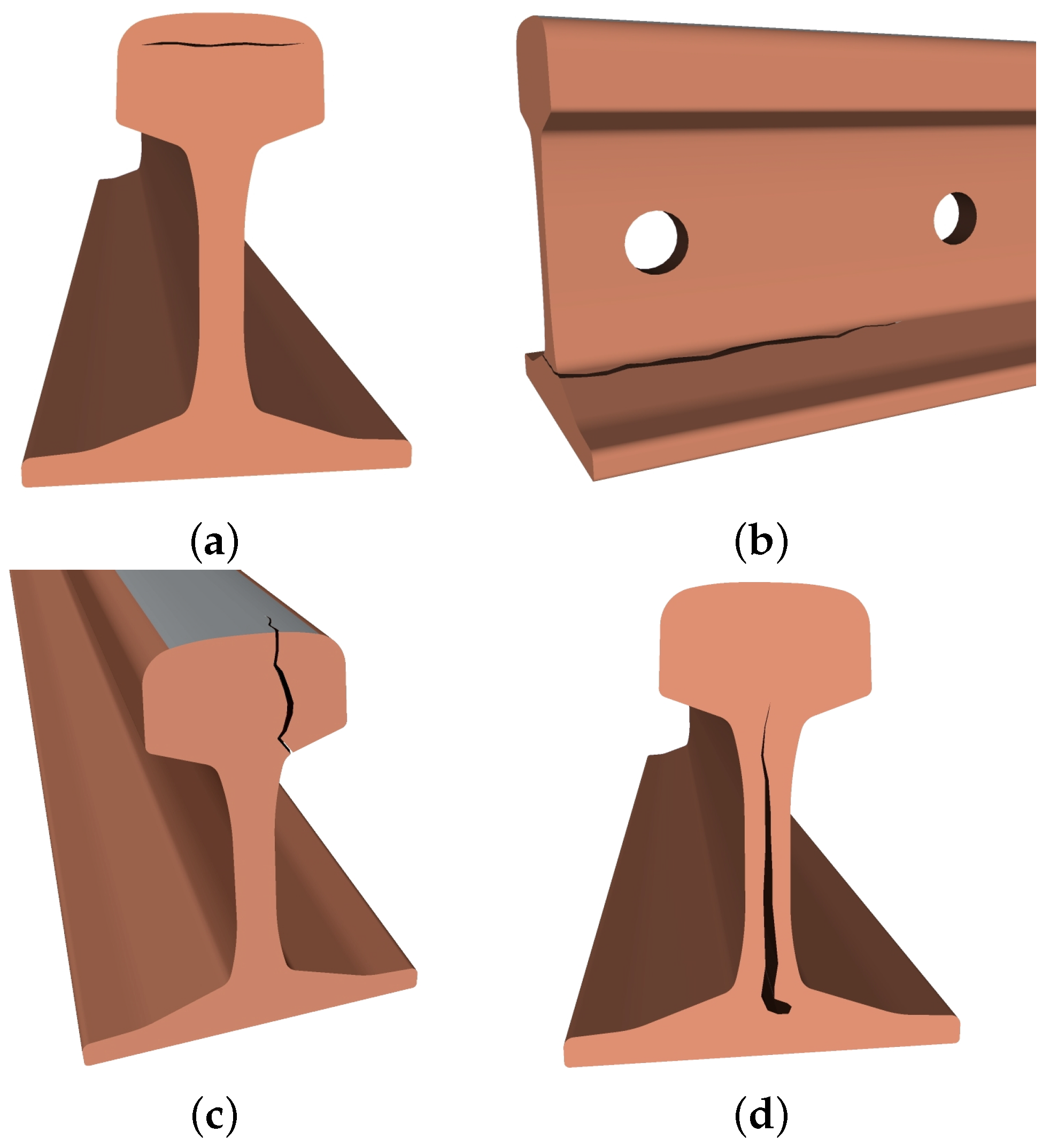
The railroad track system is very complex, and involves many interactions [8]: damage can occur anytime and anywhere. The development of defects in rails is due to uncontrolled and random processes. If not detected in time, defects can lead to rail failures, which, in some cases, happen without any previous indication. The prediction of crack growth rates and of the size of defects at failure are both influenced by various parameters [4,9]. In the following two paragraphs, we focus on the different types of defects and on the techniques that can be employed for their detection.

2.1. Rail Defects

The transverse section of a rail is represented in Figure 1. Rails in the past were joined together using fishplates; this procedure has been replaced by welding that allows for developing long and continuous stretches of rails forming a continuously welded rail.
Various classifications of rail defects are adopted in the technical literature. Following Ref. [10], a rail track defect could be either of geometry or structural type. Track geometry defects are related to the geometric conditions of tracks; track structural defects, instead, refer to ill-conditioned structural parameters of tracks (including rails [8]). In the remaining part of this paragraph, we take into consideration track structural defects only; these are divided into the three broad categories described below.

2.1.1. Rail Manufacturing Defects

Rail manufacturing defects usually comprise inclusions or incorrect local mixings in rail steel; these generate localized stresses under operative load, which, in turn, can trigger a rail failure process [1,11]. Damages of this category include transverse defects (TD) and longitudinal defects (LD) [1,12,13]. The former type of defects consists of a progressive fracture developing in the railhead parallel to the transverse direction [1] (see Figure 2); the latter type, instead, is represented by an internal progressive fracture propagating longitudinally in rails. Longitudinal defects can be further subdivided into vertical and horizontal split heads (see Figure 3).

2.1.2. Defects Due to Improper Use or Handling of Rails

Defects related to improper use or handling of rails are usually caused by train wheels spinning on rails (this produces the so-called wheelburn defect, shown in Figure 4) or by sudden train brakes [1].

2.1.3. Defects Due to Rail Wear and Fatigue

Rail wear and fatigue defects are due to wearing mechanisms of the rolling surface and/or to fatigue. Well known examples of this category are: (a) corrugation; (b) rolling contact fatigue (RCF) damages; (c) bolt-hole cracks [1].
Corrugation is related to the wearing of railhead [14] and does not compromise rolling safety, but affects both track elements and rolling stock, since it increases noise emission, loading, and fatigue [15].
Rolling contact fatigue damages are much more severe from the point of view of structure integrity, as they could lead to complete rail failure [16,17,18]. Independently of any material defect, fatigue cracks initiate on (or very close to) the rail running surface [17]. The RCF damage can be further subdivided in: (a) checking and possible spalling; (b) shelling; (c) squats (see Figure 5) [19]. The occurrence rate of RCF is proportional to the speed of the train or to its weight [1]. To counteract RCF, the damaged rail can be prematurely removed in the most severe cases or ground to remove the surface-initiated crack. The running surface can also be lubricated; however, it is believed that fluid entrapment in metal can speed up the growth of a surface-initiated crack [16].
Bolt-hole cracks appear in joined tracks; as shown in Figure 6, they originate on the surface closer to bolt-holes and propagate with a ±45 angle from the vertical up to reaching web-railhead junctions. These defects may originate from the fretting fatigue caused by the bolt shank against the surface of bolt-holes [1].
In welded rails, critical points requiring careful inspections are represented by welds (see Figure 7); in fact, internal defects of welds can affect structural integrity and fatigue performance, bringing rapid failures [5].

2.1.4. Defect Growth

The failure due to cracks of metallic structures goes through the following three phases: (a) crack initiation; (b) crack growth; (c) a subsequent quick crack growth culminating in a total fracture. Specific techniques can be used to detect cracks when they are in their earlier stages [8], so that the third phase is not reached [16]. Since defect development is due to uncontrolled and random processes or events, this process does not lend itself to a simple statistical description [4].

2.2. Rail Diagnostics Techniques

Different inspection techniques for non destructive testing (NDT) of rails are available and currently in use. These can be divided in the following classes [5]: (a) eddy current (EC)-based methods; (b) ultrasonic techniques; (c) visual inspection techniques; (d) thermal techniques; (e) radiographic techniques. These techniques require that some instrumentation is installed on a vehicle (i.e., a train or a special vehicle) to acquire the required measurements while moving on tracks.

2.2.1. EC-Based Methods

These methods include eddy current inspection and magnetic flux leakage (MFL). The method based on eddy current measures the material response to an induced electromagnetic field: the presence of a surface or near-surface defect produces a distributed electromagnetic field that can be measured. This method is contactless, but very sensitive to probe lift-off from the surface of test specimens [20]. The method based on MFL consists of magnetizing the object to be tested and in scanning its surface by means of a flux-sensitive sensor [21]. In the presence of a defect, the magnetic flux (usually contained into the magnetized test object) leaks into air [22]. This method is able to detect superficial or near-superficial transverse fissures (like RCF) but is not suited to longitudinal fissures, and its performance is influenced by the selected scanning speed [23].
The inspection speeds of the systems based on the two methods described above are limited (75 km/h for EC testing, 35 km/h for MFL) and smaller than those characterizing revenue service trains [5].
The limitations of EC inspection of rails are analyzed in Ref. [24]. Some of the most recent advances in EC-based testing of rails are illustrated in Refs. [25,26]. Finally, it is worth mentioning that a recent implementation of the MFL technology can be found in Ref. [27].

2.2.2. Ultrasonic Techniques

These comprise conventional bulk wave ultrasonics, phased arrays, and ultrasonic guided waves (A brief introduction to ultrasonic guided waves and to their propagation in rails is provided in Appendix A and Appendix B, respectively.) (UGW) techniques; the last class of techniques can be further divided into on-board and land-based systems. An introduction to ultrasonic techniques applied to rail diagnostics is given in Section 2.3.

2.2.3. Visual Inspection

Visual inspection can be exploited by a human expert walking on tracks and searching for defects, or by automated techniques. Automated visual inspection is based on video cameras, optical sensors, and custom-designed algorithms to analyze the rail surface as the diagnostic train rides over [28,29,30,31]. Test speeds can be as high as the velocity of high-speed trains [4], but only the visible surface of the rail is inspected and internal defects cannot be detected [5]. Furthermore, since detection performance is influenced by lighting conditions, proper countermeasures need to be adopted [32]. An example of a high-speed diagnostic train also making use of visual inspection techniques is shown in Figure 8 [33].

2.2.4. Thermal Techniques

These techniques exploit the change in the thermal properties of rail material in the presence of a defect. The presence of an anomaly is inferred from a single frame or from a video sequence of the temperature distribution of the surface of the considered specimen [5,34]. Some recent approaches are illustrated in Refs. [35,36].

2.2.5. Radiographic Techniques

Radiography is the only technique able to analyze visually the interior of a rail or a weld. This method can detect cracks, flaws, and thickness reduction in detail, but has safety hazard concerns, is expensive, and time consuming. For these reasons, it is often used to analyze rails; only after that have other NDT techniques detected a specific problem [5].

2.2.6. Track Circuits

Track circuits are systems used to detect the presence of a train in a stretch (section) of track by means of an electrical current. A transmitter and a receiver placed at the two ends of the considered track section are exploited. In the absence of trains, an electrical signal flows through the rails from transmitter to receiver. On the contrary, when a train enters into the track section, its wheels short-circuit the pair of rails, so that the signal sent by the transmitter is unable to reach the receiver and the section status becomes busy. An occupied section is also detected if a complete rail failure occurs, since the electrical continuity is interrupted. The main problem of track circuits is represented by the fact that they are able to detect a rail failure only if the electrical continuity of the associated circuit is interrupted; consequently, early-stage cracks are not detected [37].

2.3. Defect Detection Techniques Based on Ultrasonic Waves

Detection techniques based on ultrasonic waves are divided into three main categories [5]: (a) conventional ultrasound, (b) phased arrays, and (c) guided waves ultrasound.

2.3.1. Conventional Ultrasonic Techniques

If these techniques are employed, the railhead is scanned by means of ultrasonic beams: defects are detected by measuring the reflected or scattered energy. The presence of a defect, along with its location and severity, is inferred from the amplitude of the resulting reflections and their arrival times [23]. The employed ultrasonic transducers are contained within a liquid-filled tire; this allows for improving signal quality by reducing the acoustic mismatch between rail steel and air. For the same reason, water is sprayed between the wheel containing the ultrasonic probes and rails [4]. Although ultrasonic testing is capable of inspecting the whole railhead [38], it has the following limitations: (a) limited car speed in ultrasonic inspection [16] (in practice, the achievable test speeds can be as low as 15 km/h [4] and, consequently, inspection has to be accomplished outside the operation period of commercial trains [1]); (b) shallow crack shadowing [13,16] (small shallow cracks can shade more severe and deeper cracks by reflecting ultrasonic beams [1]); (c) false defect detection [1] (this slows down inspection operations).
The ultrasonic testing vehicle “us1-Galileo” employed by the Italian railway infrastructure manager, Rete Ferroviaria Italiana (RFI), is shown in Figure 9.

2.3.2. Phased Arrays

Phased arrays use multiple ultrasonic elements and electronic time delays to generate beams by exploiting constructive and destructive interference. Phased arrays provide ultrasonic beams that can be steered, scanned, swept, and focused electronically [39].

2.3.3. Guided Waves

In an effort to overcome some of the technical problems associated with ultrasonic wheel inspections, some research groups are investigating ultrasonic guided waves for rail inspections. Different types of guided waves can propagate in any bounded medium. Inspection tests can be accomplished in pulse-echo mode; this means that an ultrasonic transducer is employed to transmit a pulsed guided wave along the structure of interest and that the presence of defects or other structural features is inferred from analyzing the returning echoes sensed by the same transducer [7]. Operation in pitch–catch mode can be also employed; in this case, a transmitter generates a guided wave in the waveguide and a receiver (i.e., a different transducer, placed at the other end of the sample) is employed to detect the incoming wave. If a defect reflects a portion of the transmitted energy, the received signal is weaker than that observed in pristine waveguide conditions; this allows for detecting the presence of defects [40].
Ultrasonic guided waves offer the following advantages [41]: (a) guided waves propagate along (rather than across) rails, and are ideal for detecting critical TDs, even if they are relatively insensitive to parallel fissures [42]; (b) guided waves allow for improving inspection coverage, thereby relaxing limits on the maximum achievable speed (if the inspection equipment is installed on-board a moving vehicle); (c) guided waves can travel underneath shelling and still interact with internal defects, since they penetrate a finite depth of the surface of rails; iv) guided waves can penetrate alumino-thermic welds, hence potentially targeting weld cracks and discontinuities, since they travel in the mid-frequency range (say, in the 20 kHz–1 MHz range).
Unluckily, the complicated propagation behavior of guided waves cannot be easily managed [43]. In fact, ultrasonic guided waves, especially in complex waveguides such as rails, express a multi-mode character (many modes can propagate simultaneously) and a dispersive character (the propagation velocity depends on frequency) [7]. In practice, tens of different modes can be observed in the employed frequency range; moreover, the dispersion curves characterizing this propagation phenomena are very complicated [43], as it can be easily inferred from Figure 10.

3. Systems for Rail Defect Detection Based on Ultrasonic Guided Waves: Classification

Substantial research efforts have been devoted to the study of systems exploiting ultrasonic guided waves for the detection of rail defects. More specifically, the following two broad categories of systems have been investigated:
  • On-board systems [40,45,46,47,48,49]-The measurement equipment is embarked on board a moving vehicle (e.g., an inspection cart), allowing for scanning the head of the rails on which it is riding. The detection of defects in the scanned rails is achieved through a pitch–catch mechanism. Initial implementations were based on an active approach, in which a source of ultrasounds was used to inject UGW into the rails, and sensing was accomplished through an array of transducers. More recent implementations adopt a passive approach, in which the ultrasonic excitation is generated by the rolling wheels of the moving vehicle. The approaches based on on-board systems have been promoted, among others, by the Experimental Mechanics & NDE Laboratory of the University of California, San Diego, USA.
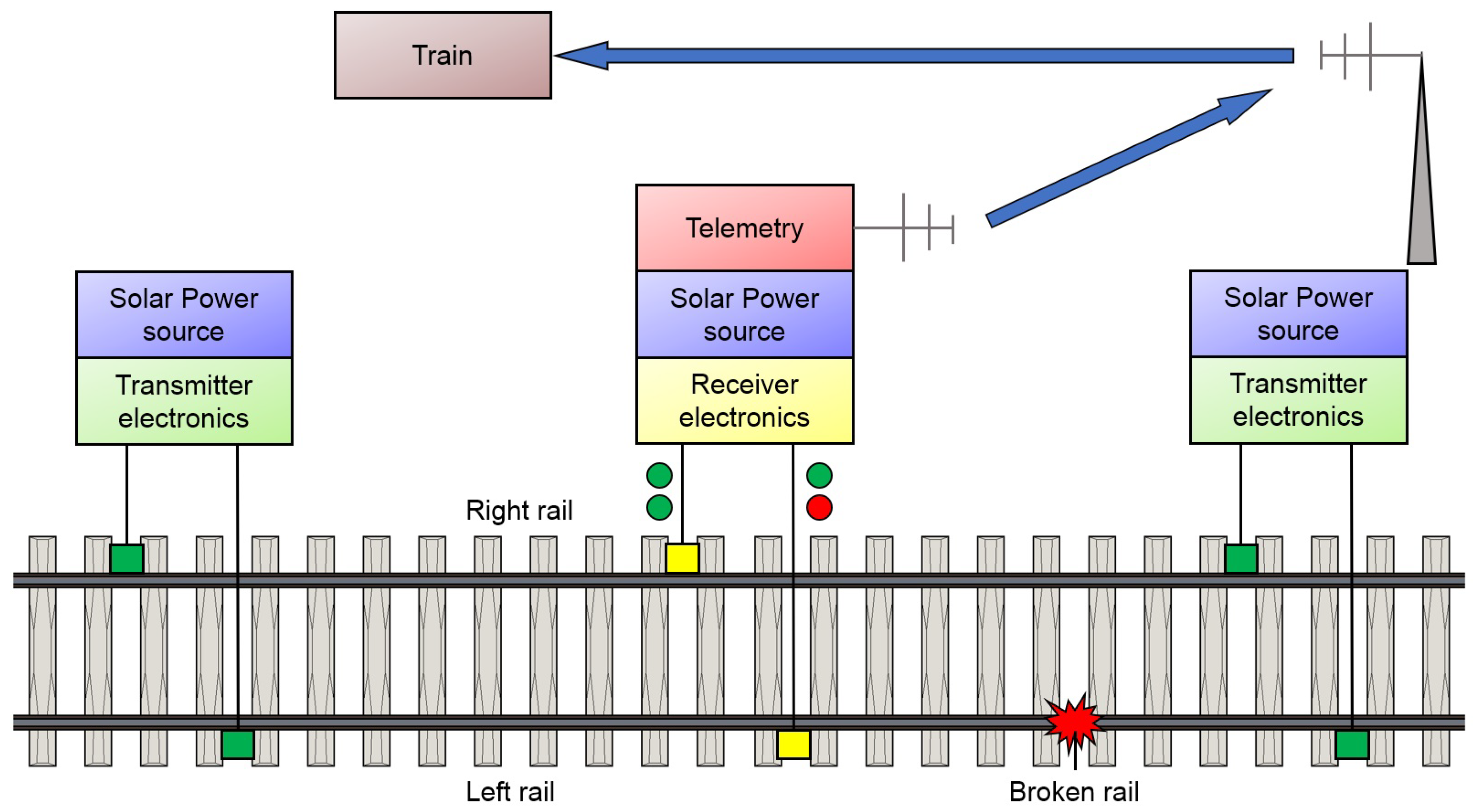
  • Land-based systems [9,50,51,52,53,54,55,56,57,58,59,60,61,62,63,64,65,66,67]-The employed equipment is placed on the ground near to the railway infrastructure, and its actuators and sensors are attached to the rails under test. The detection of defects in the rails is achieved through a pulse-echo approach. A lot of contributions about this topic have been published by the Sensor Science and Technology Department of the Council for Scientific and Industrial Research, South Africa. The ultrasonic broken rail detection (UBRD) system has been developed by this institution and put in use on the Oreline in South Africa to detect the presence of a fully broken rail; the system is evolved to implement an early defect detection system. In recent years, important results in this research field have been achieved by two Chinese research groups. In fact, significant contributions about the best methods to excite and detect propagation modes in a rail, and about feasible methods for rail defect location have been published by various researchers working at the Beijing Jiaotong University (School of Mechanical, Electronic, and Control Engineering, and Key Laboratory of Vehicle Advanced Manufacturing, Measuring and Control Technology). Moreover, an electronic system able to efficiently excite ultrasonic guided waves in rails has been developed by various researchers working at the Xi’an University of Technology (Department of Electronic Engineering).
In the remaining part of this manuscript, both categories of systems are taken into consideration. In particular, the architecture of these systems is described in Section 4. Section 5, Section 6 and Section 7 are devoted to the implementation of on-board approaches, to that of the UBRD system, and to the evolution of the UBRD system towards early defect detection and monitoring. In Section 8, commercial projects like RailAcoustic (by Enekom), or university studies, like those accomplished by the Beijing Jiaotong University or the Xi’an University of Technology are summarized. Finally, various results about the performance provided by each of the considered systems are illustrated in Section 9.

4. Systems for Rail Defect Detection Based on Ultrasonic Guided Waves: Architecture

In the technical literature, various architectures have been proposed for on-board or land-based systems for rail defect detection based on UGWs. In this section, some essential features of the available technical options are illustrated.

4.1. On-Board Systems

Over the years, active and passive detection strategies have been proposed for on-board systems. The main characteristics of the systems employing such strategies can be summarized as follows:
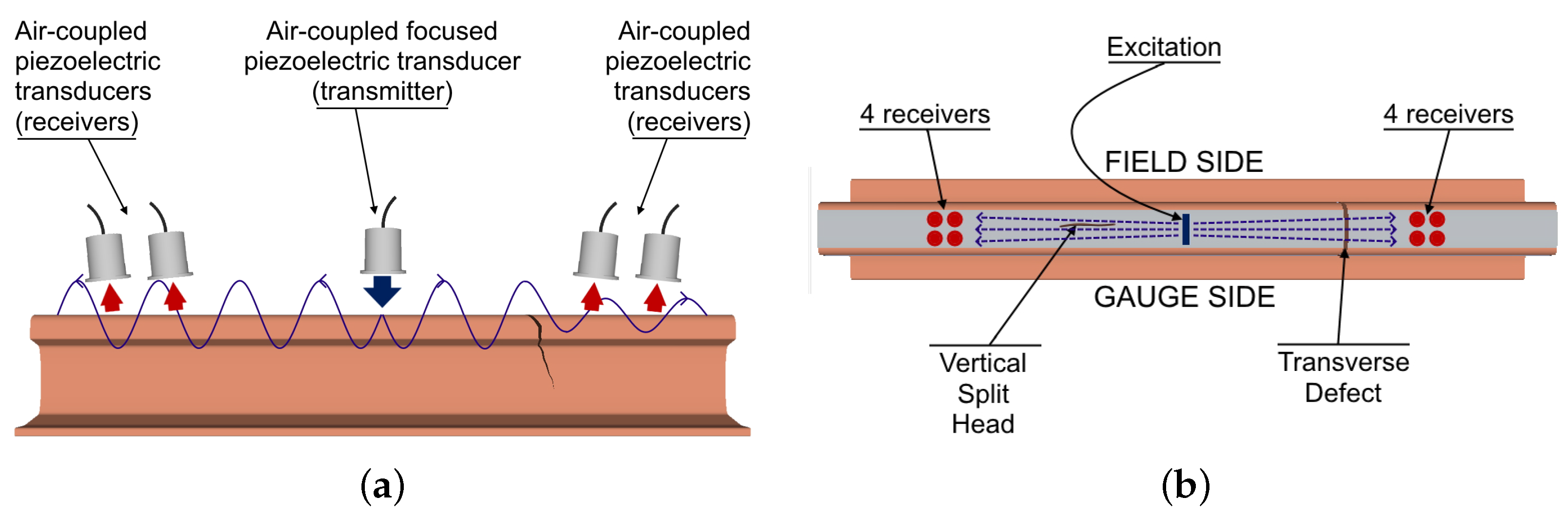
  • An active rail inspection system is able to detect surface-breaking cracks and internal defects located in the railhead. It is based on UGWs and air-coupled contactless probing. Both the transmission of test signals and their reception are accomplished by means of air-coupled piezoelectric transducers arranged in a pitch–catch configuration. The use of a laser transmitter has been also investigated [40]; however, this option has been judged too costly and is potentially hard to maintain. In an active system, receivers are arranged in pairs and placed at the two sides of the transmitter: this allows for implementing a differential detection scheme. The system output, after data analysis, is represented by the so-called damage index (DI), exhibiting peaks in correspondence of discontinuities (i.e., of potential defects) in rails. In recent years, the use of laser technology for both exciting UGWs in rails and sensing them has been investigated [68,69]. In this case, non-ablative laser sources are used to generate a guided tensional wave system in the rail; the response to such a system can be sensed by means of a rotational laser vibrometer.
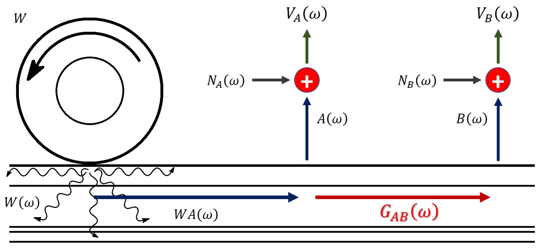
  • A passive rail inspection system aims at estimating the acoustic transfer function of rails; the excitation is represented by the rolling wheels of the moving instrumented train [48]. When a train is in motion, its rotating wheels generate a continuous dynamic excitation of the rail. Such an excitation is uncontrolled, non-stationary, and difficult to characterize [48]. Therefore, in this case, the challenge to be faced is to generate a stable rail transfer function that is not affected by the excitation [49]. The presence of a discontinuity in the rail can be inferred from the estimated transfer function, using again the DI indicator.

4.2. Land-Based Systems

The UBRD is a broken rail detection (BRD) system, designed to continuously detect full breaks in rails [50]. Its transducers are tied to the rail and allow for monitoring a span of up to 1 km of track in pitch–catch mode. This system has been already installed on 841 km of tracks in the high-haul Oreline network in South Africa [51,52]. The system architecture is represented in Figure 11; its operation is based on a simple transmit–receive confirmation protocol. As long as a reliable reception of the ultrasonic signal generated by the transmitter is possible, the integrity of the rail is verified; otherwise, an alarm is set [50,53].
The developers of the UBRD system are studying how UGWs can be exploited to detect and monitor a growing defect, and how specific guided modes can be excited in a rail. The use of techniques for the excitation of guided waves different from those based on piezoelectric transducers have been investigated. For example, the use of electromagnetic acoustic transducers (EMATs) has been taken into consideration [55]. In the meantime, the reflection characteristics of defects and their dependence on time and environmental conditions are under evaluation [9,56,57,65].
In principle, UGWs have the potential to monitor a long span of a waveguide using permanently installed transducers in pulse–echo mode. The same transducer array is used to generate the ultrasonic wave and then to measure the echo generated by the wave reflection on a defect. A continuously welded rail is a perfect example of such a waveguide and, as a matter of fact, defects (and welds) act as reflectors for guided waves. A system based on this approach is able to detect the presence of a defect, and to estimate its magnitude and location. These results are achieved by monitoring the echoes coming from defects (defect presence), measuring their amplitude (defect magnitude) and the time-of-flight required by the transmitted wave to travel back and forth from the transducer to the defect (defect location) [51].
An important advantage offered by land-based solutions is represented by the fact that monitoring can be accomplished in near real-time, so that defect growth can be analyzed over time and an alarm set only when a crack assumes a potentially critical size [9,65].
Further details about the architecture of the UBRD system are provided in Section 6. In Section 7, its evolution towards an early defect detection system is described. Other projects or studies about land-based systems are illustrated in Section 8.

5. Implementation of On-Board Systems

In this section, the implementation of on-board systems is described in detail; both active and passive approaches are considered.

5.1. Active Approach

5.1.1. Hardware Configuration

The configuration adopted in the active on-board system is shown in Figure 12: a single focused transmitter and four pairs of receivers are fixed to a frame which is in turn attached to a cart [40,45,47]. The lower active surface of the transducer is separated from the upper surface of the rail; their distance is known as lift-off and is on the order of a few centimeters for both the transmitter and the receivers. The transmitter feeds the top of the rail surface with a narrowband toneburst signal (a Hanning-windowed sinusoid); it has a tunable repetition rate (representing the frequency of the excitation and related to spatial resolution). This results in a (repeated) multimodal guided wave that propagates symmetrically with respect to the excitation line. The receivers detect the guided waves leaking into the surrounding air; for this reason, they are tilted according to Snell’s law.

5.1.2. Defect Detection Principles

The pair of receivers placed at the two sides of the transmitter are employed in a differential detection scheme; this compares the strength of the signal received at both sides. If an internal flaw is present on one side of the transmitter or on the other one, the transmitted wave is scattered and the outputs of the receiver pair are unbalanced. Some strength-related metrics are extracted from the received waveforms to generate a “feature supervector”; in practice, this is obtained by combining the “feature vectors” provided by the two receivers. These metrics are listed in Table 1, in which the symbols P k P k x and R M S x denote the mean peak-to-peak and root-mean-square, respectively, of the quantity x [46].

5.1.3. Signal Processing

The received signal needs to be properly processed (and, in particular, denoised) to overcome the inherently low signal-to-noise ratio (SNR) of air-coupled piezoelectric sensors [40]. A multivariate outlier analysis (MOA) is used to compensate for the natural signal variations expected during the test; the final result is represented by a damage index (DI) computed at each test position. Defects are detected by an high value of DI, i.e., by an unusually large discordancy index from the “normal” baseline of the rail. The DI is represented by the Mahalanobis squared distance discordancy metric D ζ of a MOA [46], which is defined as
D ζ = x ζ x ¯ T · K 1 ·   x ζ x ¯ ,
where x ζ is the potential outlier vector, x ¯ is the mean vector of the baseline, K is the covariance matrix of the baseline, and ( · ) T represents the transpose operator. A new observation is classified as an outlier if the corresponding value of D ζ is higher than a proper threshold, previously established [45].
To reduce the probability of false alarms due to the occurrence of isolated noise-related high peaks in the DI trace, system redundancy can be exploited [46]. When scanning a defect, the presence of a real crack should result in multiple peaks in the observed trace. Therefore, a peak is detected by the system only when a given number of DI values exceeds the above-mentioned threshold.

5.1.4. Reverberation of Airborne Signals Caused by an Acoustic Mismatch

The presence of reverberations of the airborne waves between the transmitter and the top of the excited rail has been found. This phenomenon is caused by the unavoidably high acoustic impedance mismatch between the air medium and the solid boundaries of the rail steel and of the piezoelectric transducer. The strong intensity of the reverberations affects the detection of acoustic waves traveling through the rail steel associated with the presence of rail defects. Although time gating can effectively separate the signal of interest, a lower SNR is observed when the repetition rate (i.e., the frequency of the excitation) is sufficiently high such that the airborne reverberations from a previous excitation overlap with the waves of a new excitation. This limits the test speed to ∼1.6 km/h (∼2.4 km/h when a slightly worse SNR is acceptable) because of the required spatial resolution. The most effective solution developed for this problem until now consists of inserting a sponge between the transmitter and the rail to attenuate the airborne reverberations. The main drawback of this solution is represented by the fact that the sponge has friction with the rail, and this raises the noise level affecting the received waves as the train speed increases; in practice, a reliable signal detection is possible up to 24 km/h [47]. Some test results are illustrated in Section 9.1.

5.2. Passive Approach

5.2.1. Hardware Configuration

In this case, as illustrated in Refs. [49,66], the sensing head is made of two receivers, denoted A and B, separated by a known distance; both are sensitive only to waves propagating unidirectionally (from left to right in Figure 13). The sensing head is mounted on a beam rigidly connected to the front-axle of the test car; similarly as in the active approach, contactless probing is employed. The sensors are tilted with respect to the rail surface (according to Snell’s law) to best capture the leaky surface waves propagating in the railhead. The orientation of receivers ensures directional sensing of the waves excited by the wheels located on only one side of the arrays (front end), with virtually no sensitivity to waves propagating in the opposite direction (i.e., to reflections or waves excited from the wheels located to the other side of the arrays’ back end).
Data are continuously recorded for the entire duration of the test [49]. A tachometer logic pulse marking the spatial position of the test car and GPS positioning are recorded, in addition to high-speed camera videos of the tested rail to verify the presence of visible discontinuities when the prototype detects an anomaly [48].

5.2.2. Defect Detection Principle

In this case, defect detection requires the estimation of the time domain Green’s function G A B t between the two receivers A and B, without prior knowledge of the source excitation spectrum. This function represents the response of the test object measured a B from an impulse excitation at A. If the frequency domain Green’s transfer function G A B ( ω ) can be estimated, discontinuities in the rail (such as defects) can be detected by means of a procedure similar to that illustrated for the pitch–catch ultrasonic guided-wave approach. In fact, discontinuities can be perceived as a change in the structural impulse response, G A B t , obtained from G A B ω through an inverse Fourier transform. In terms of defect detection, as long as the reconstructed Green’s function is stable during a test run, successful passive structural inspection becomes possible.
The estimation of the Green’s function is based on the computation of the ensemble averaged cross-power spectrum between the output and the excitation, normalized to a modified ensemble averaged auto-power spectrum of the excitation. The following assumptions are made: (a) the system is linear and piecewise stationary, so that the statistics of the excitation W ω do not change in the observation interval; (b) the noise terms are uncorrelated, have a zero DC component, and tend to zero on average, thus enabling for separating the useful signal component from noise. The function G A B ω is estimated by computing the deconvolution of the cross and auto power spectra. In fact, the spectra of the responses at A and B can be expressed as
V A ω = W ω   ·   W A ω   ·   A ω + N A ω
and
V B ω = W ω   ·   W A ω · G A B ω   ·   B ω + N B ω ,
respectively; here, V A ω V B ω is the response measured at receiver A (B), W ω is the wheel excitation spectrum, W A ω is the transfer function of the rail between the wheel and the transducer at A, A ω ( B ω ) is the frequency response of the receiving sensor A (B), N A ω ( N B ω ) is the uncorrelated noise originating from the environment at A (B) (see Figure 13).
Based on Equations (2) and (3), it can be shown that [49]
Cross Power = W ω 2 W A ω 2 G A B ω
and
Auto Power = W ω 2 W A ω 2 ,
in which the symbol 〈〉 represents the ensemble average operator.
By using Equations (4) and (5), the frequency Green’s Function between the two receivers is computed as
Cross Power Auto Power = W ω 2 W A ω 2 G A B ω W ω 2 W A ω 2 = G A B ω .
Then, the time domain Green’s function can be evaluated by taking the inverse Fourier transform from the left-hand side of the last equation, i.e., as
G A B t = 1 2 π + G A B ω e j ω t d ω .
The last integral is computed in an approximate fashion through an inverse fast Fourier transform (IFFT).

5.2.3. Data Processing

The employed data processing is sketched in Figure 14. In each run, the recordings from receivers A and B are first amplitude-clipped to within the ±3 standard deviations to mitigate the effects of isolated spikes in the passive reconstruction of the impulse response G A B t . Then, the resulting signals undergo fast Fourier transform (FFT) processing, so that cross and auto power spectra and the transfer function G A B ω can be computed. Finally, the time domain Green’s function G A B t is evaluated by (a) averaging the function G A B ω over four sensor pairs and (b) accomplishing band-pass filtering and IFFT processing. An outlier analysis is implemented in order to compute the DI related to the strength of the reconstructed transfer function; this issue has already been discussed in Section 5.1.3, when describing the active method for rail defect detection. The computation of the DI allows for normalizing the available data, thus mitigating the normal (baseline) data variability occurring in each run [48,49].

5.2.4. Trade-Offs

The impulse response G A B t is the result of the constructive interference of the wave modes continuously generated by the wheel excitation and propagating in the rail between the receivers. The constructive interference and, hence, the rate of convergence of the passively reconstructed transfer function (or, equivalently, its SNR) benefit from signal averaging. For this reason, time windows involving long recordings are preferred. Note, however, that, since both the transmitters and the receivers are moving along the test specimen (rail), the stationarity of the reconstructed transfer function can be guaranteed only in a fixed position. For this reason, a good trade-off needs to be achieved between the long recording time required by the averaging process and the stationarity (related to spatial localization) of the transfer function that calls for shorter observations. This explains why the test speed has to be properly selected: the higher the velocity is, the shorter the recording time is, ensuring a sufficiently accurate spatial localization [48].
Some test results are illustrated in Section 9.2.

6. Land-Based Systems Implementation-Premise: Ultrasonic Broken Rail Detector (UBRD)

In this section, we focus on the implementation of land-based systems. Since the topic is wide, the description of these systems is provided in three consecutive sections, each focusing on specific technical issues, as already mentioned at the end of Section 4.

6.1. UBRD Hardware Configuration and Generated Signals

Transmitters and receivers of the UBRD system are interleaved, as illustrated in Figure 15. Every receiver is able to acquire signals coming from both directions of the rail; to identify the exact orientation, the transmitted signals consist of different burst sequences depending on the transmitter. In fact, as it can be easily inferred from Figure 16, each transmitted sequence consists of a number of pulses spaced by a given burst repetition interval (BRI) and is repeated at a specific interrogation interval (II). This avoids the overlap at one receiver of burst trains coming from adjacent transmitters for extended periods. For such reason, receivers are also individually configured to recognize specific pulses as arriving from either the up or down direction depending on the settings of adjacent transmitters. Note also that each signal does not reach a receiver far from its transmitter because of the attenuation due to the propagation medium [50,53].

6.2. Defect Detection Principle and Employed Signal Processing Method

The transducers of each transmitter generate an acoustic signal that propagates through the rail; this signal travels in both directions and can reach receivers located at a significant distance from the transmitter. The received signals are filtered, amplified, and processed. Rail integrity between the transmitter and each receiver is confirmed as long as an acceptable signal is received. If a clean break occurs in the considered stretch of rail, the corresponding receiver will no longer be reached by the transmitted signal and will generate an alarm [50,53]. Receivers detect valid signals on the basis of specific criteria concerning signal frequency, burst length, burst repetition interval, and burst train continuity.
Severe continuous noise (such as that generated by an approaching train) at a receiver will affect signal detection, regardless of the efficiency of the employed detector. Under such circumstances, the receiver will generate the message “train in section”, will stop processing its input signals, and will remain idle until the noise intensity decreases; then, it will return to its normal conditions.
This system is commercialized under the name “RailSonic-ultrasonic broken rail detector”. The system is not classified “Fail Safe”, although in Ref. [50], it is claimed that many fail safe principles have been incorporated in order to correctly detect most of equipment failures; this allows for correctly identifying these events and are, at the same time, to avoid false alarms.

6.3. UBRD Updates

To update the UBRD, a new piezoelectric transducer has been developed, thanks to numerical modeling and measurement techniques. This improvement and the use of new digital signal processing techniques have been incorporated into a new version of the UBRD system that allows for doubling the distance between transmit and receive stations [51].
Yuan et al. have proposed a method to integrate the UBRD system with a train detection (TD) system [54]; the resulting system is able to distinguish the following three different track conditions: free, busy, and broken rail. This is made possible by extracting, from the ultrasonic guided waves, the following three features: (a) the RMS value and (b) the energy in the time-domain; (c) the frequency component with the highest amplitude in the frequency domain. In addition, temporal and spatial dependencies of the signals are taken into consideration. High-level signal processing techniques, such as deep learning algorithms, are also employed to deal with varying environmental situations and conditions. The suitability of this approach has been assessed through experimental tests.
In Ref. [67], the same authors as Ref. [54] have proposed to exploit the variational mode decomposition (VMD) algorithm to de-noise and reconstruct ultrasonic guided wave signals. The VMD method is a quasi-orthogonal signal decomposition technique for non-recursively decomposing a multi-component signal into a finite number of compactly band-limited intrinsic mode functions (IMFs). The VMD algorithm is used to decompose ultrasonic guided wave signals into the fundamental, harmonics, interharmonics, and non-stationary disturbances, and can be used in conjunction with the method developed in Ref. [54].

7. Land-Based Systems Implementation-Evolution: Early Rail Defect Detection Capability

An experimental system able to monitor an operational rail track by means of ultrasonic guided waves has been proposed in Ref. [65]. In this section, the prototype and the methodologies adopted to process and analyze the available data are illustrated. Moreover, various technical problems and the solutions developed to solve them are briefly described.

7.1. Introduction

Numerous types of defects appear in rail tracks, and multiple parameters affect the prediction of crack growth rates and of the defect size at failure [9]. In principle, the baseline subtraction method could be used to detect the insurgence of a defect over time. Baseline subtraction is based on the idea of feeding a system in a given condition with a known excitation, measuring its response, and storing it as a baseline. Each and every modification in the system reflects in a change in its response to the same excitation. Therefore, in principle, the occurrence of any change potentially due to a defect can be detected by comparing each new response to the baseline. In practice, however, it is not easy to establish if such a change is caused by a defect or by a variation of other parameters affecting the system response to the considered excitation. In fact, it should be always kept in mind that, in harsh environments like rail tracks, any variation observed in the propagation conditions of ultrasonic signals can also originate from changes in environmental and operating conditions (EOCs); these conditions include, for instance, temperature, train passing, or maintenance operations [51].
The continuous monitoring of a rail track can provide better performance results in terms of defect detection probability than a single inspection, though it is influenced by the EOC. In this case, the most important technical challenges are: (a) the development of a permanently installed UGW-based monitoring system for rail defect detection at a reasonable cost per kilometer of track; (b) the development of a defect detection technique able to reliably operate in the presence of real EOCs. Of course, if a suitable facility is unavailable, tests can be performed on operative tracks. The problem is that damaged sections of rails are removed as soon as defects are detected; furthermore, rails must not be damaged or altered. Consequently, it is impossible to test the available prototypes on real cracks: their performance is assessed by using welds or glued masses, both acting as reflectors for guided waves [9].
Different problems must be addressed in order to achieve an effective automatic monitoring system for rail damage detection. In particular, the following specific technical issues should be investigated: (a) the behavior of a defect growing over time; (b) the influence of the selected transducers on the quality of the received signal; (c) the influence of the changes in rail properties on the propagation of guided waves and the parameterization of these changes; (d) the influence of time varying EOCs on wave propagation and the methods for compensating for these variations; and (e) the identification of the defect detection algorithm and the use of proper methods for assessing its performance.

7.2. Monitoring Set-Up

In this section, the hardware and software architecture of the system illustrated in Ref. [65] are briefly described.

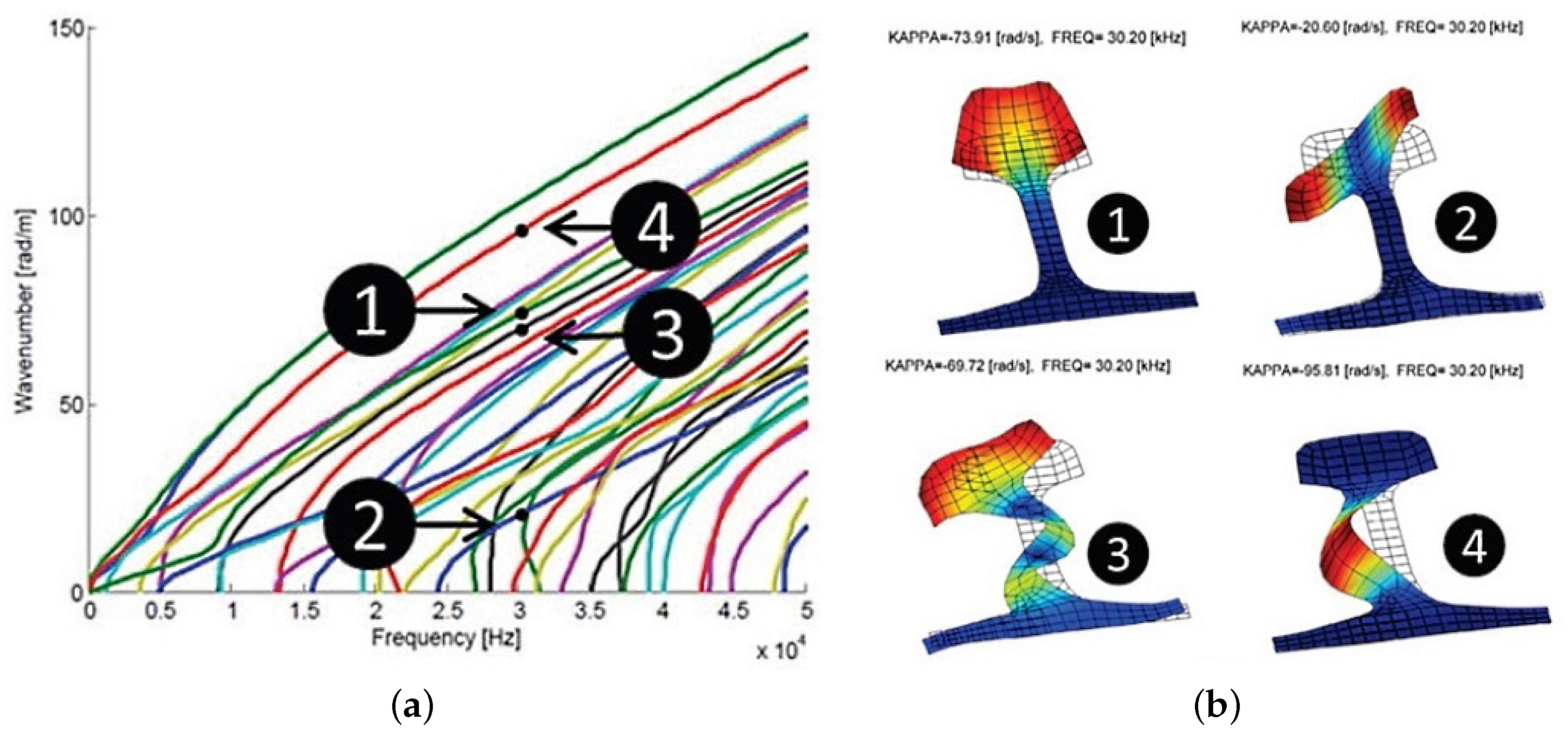
7.2.1. Selected Modes for Guided Wave Propagation

Numerical simulations based on the semi-analytical finite element algorithm (SAFE) have allowed for identifying a guided wave mode suited for the detection of defects in rails. This mode propagates with relatively small attenuation and dispersion, and it is strongly reflected by transverse defects in the railhead. It can be excited by a transducer attached under the railhead. The identified mode, used for both transmission and reception, is a symmetric mode that has motion in the vertical axis while propagating along the longitudinal direction moreover with the energy mainly concentrated in the railhead [65]. The SAFE is a popular method developed to solve wave propagation problems in waveguides. It can be employed to compute the dispersion curves of the modes that propagate along a waveguide characterized by an arbitrary cross-section. It has been shown that, in the analysis of waveguides that are infinitely long in one direction, SAFE achieves better accuracy than finite element (FE) methods at a lower computational cost. A detailed description of this method can be found in Ref. [70].

7.2.2. Monitoring System Hardware and Software

Two piezoelectric transducers, forming an array and attached under the railhead, are employed to perform pulse-echo measurements [9]; the sandwich piezoelectric transducers have been designed to effectively excite the selected mode of propagation around 35 kHz [65]. The distance between the axes of the transducers has to be equal to one quarter of the wavelength of the excitation signal.
Two specific technical problems have been faced in system design [56]. The first problem is represented by the slightly different resonant frequencies of the two transducers; this is due to the tolerances characterizing the manufacturing process. Moreover, the transducer performance may change differently over time and, in the presence of temperature variations, thus causing asymmetric changes in the measured reflections and replicas. A possible solution to this problem is to independently scale the reflections from the positive direction and from the negative one, so that the difference in their amplitudes can be compensated for; this requires the estimation of the attenuation in both directions. The second problem is represented by the presence of multiple replicas originating from reflections; phased array processing can be exploited to solve this problem.
The experiments were performed on a section of tracks consisting of rails joined by aluminothermic welds. Transducers and the artificial defects mentioned in Section 7.2.3 have been placed far from the joints.

7.2.3. Behavior of a Defect during Time

The behavior of a defect over time can be analyzed by using a deteriorating defect emulator, such as a glued mass. The reflection of a glued mass deteriorates quickly over time, thanks to the stresses caused by trains and to the progressive corrosion of the rail under the glue. A monotonically increasing defect, similar to a growing crack, can be simulated if the reflected signals recorded during the time window starting at the installation of the defect emulator and ending at its detachment are time reversed [9]. The size of the mass representing the crack has to be selected to provide a realistic reflection, such as a small transverse crack in the railhead. Reflections from rail welds can provide a useful reference during testing; furthermore, if these welds can be detected, it is believed that a crack can be found well before it reaches a critical size [44].

7.3. Signal Pre-Processing

The employed excitation signal is a Hanning-windowed tone burst signal whose center frequency is equal to 35 kHz. The measurements are acquired by exciting one piezoelectric transducer, acquiring the response of both transducers of the array, and then repeating the process by exciting the other transducer. This cycle is repeated k times, and the average of the k acquired measurements is stored as a new signal in the measurement set, which consists of four time domain signals.
Noise from passing trains has to be avoided since it would overwhelm the useful signal. For this reason, the system first senses the presence of train noise and proceeds with the acquisition only in its absence; otherwise, it delays its acquisition. In the observation interval m, distinct sets of measurements are recorded.
Before defect detection or monitoring, the acquired data must be pre-processed to compensate for unwanted effects. The pre-processing steps are illustrated in Figure 17 and described in the following sub-sections. Data pre-processing involves (a) phased array processing; (b) dispersion compensation; (c) signal stretching and scaling; (d) signal reordering. These steps are required to discriminate the direction of the reflections, to reduce the influence of dispersion and to compensate for some of the changes occurring in EOC, respectively. Signal reordering accounts for the use of a mass as a defect emulator: the mass, in fact, behaves in a reversed time order with respect to a crack (see Section 7.2.3).

7.3.1. Acquired Signals

The impact of noise in the received signal can be reduced by band-pass filtering, making easier the task of detecting the reflections in the steps to follow. The center frequency and bandwidth of the filter can be set to be the same of the excitation signal. During pre-processing, the signals are converted to the frequency domain.

7.3.2. Phased Array Processing

An array of transducers allows for exciting a specific mode in a desired direction of propagation, even if the array is composed of two transducers only. This result is obtained by feeding both transducers with excitation signals characterized by a small difference in delay or phase. The phase difference depends on the wavelength of the propagation mode selected at the transmission frequency and on the axial distance between the two transducers. The same idea can be exploited at the receive side; in fact, if a phase shift is applied to the signal acquired by a transducer, the energy associated with the desired mode and originating from the desired direction can be captured. It is worth noting that a perfect cancellation is impossible, since other modes characterized by different wavelengths are transmitted and received in both directions. This problem can be mitigated by increasing the overall number of transducers forming the array.
Phased array processing can be applied to the full matrix of signals acquired from an array of transducers, as explained by Wilcox in Ref. [71]. The acquired time signals are converted to the frequency domain and, after processing, are converted back to the time domain. When the first (second) transducer is excited, the responses acquired by both transducers are stored in the first (second) column of the measured displacement matrix
V ω = V 11 ω V 12 ω V 21 ω V 22 ω ;
Here, V i j ω is the spectrum of the response of the i-th transducer in the array (with i = 1 and 2, if the array consists of two transducers only) in response to the excitation injected through the j-th transducer (with j = 1 and 2, if the array consists of two transducers only).
The analysis of different combinations of transmitted and received propagation modes requires the computation of mode shape matrices. Each column of the mode-shape matrix refers to the displacement of a mode at each of the transducer locations. The mode shape matrices for an array of transducers in a 1D waveguide (such as a rail) contains both mode shape and phase information according to the axial position of the associated transducer, for each mode in every possible direction [71]. Since it may happen that the modes selected for receive processing are different from those chosen for transmit processing, two mode shape matrices are required, one for reception and the other for transmission (denoted R ω and T ω , respectively). If the same modes are selected for reception and transmission, then R ω = T ω . The coefficients of these matrices are computed through a SAFE analysis of the rail.
If the mode shape matrices R ω and T ω , and the measured displacement matrix V ω (8) are known, the contributions of the different modes to the received signal can be computed. The spectrum α ω of the overall response is evaluated as
α ω = R ω 1 V ω T ω * 1 = α r 1 t 1 ω α r 1 t 2 ω α r 2 t 1 ω α r 2 t 2 ω ;
Here, the spectrum α r 1 t 1 ω ( α r 2 t 2 ω ) describes the transmission and reception in the forward (backward) direction, whereas α r 2 t 1 ω ( α r 1 t 2 ω ) is the transmission in the forward (backward) direction and the reception in the backward (forward) direction. Note that (a) α r 1 t 1 ω is ideally equal to zero; (b) the presence of reflections from features (defects, welds, and any other element reflecting back guided waves towards the array of transducers) in the forward (backward) direction are inferred from α r 2 t 1 ω ( α r 1 t 2 ω ); (c) proper calibration factors can be introduced to compensate for the different sensitivities of the two transducers (see Section 7.2.2).

7.3.3. Dispersion Compensation

Even if a mode characterized by a small dispersion is selected, the effects of this phenomenon can be appreciable in the presence of a long propagation range. Dispersion compensation can be performed by exploiting the algorithm developed by Wilcox [72] and the dispersion data evaluated by means of the SAFE method in the considered scenario. The compensation process allows also for converting the received signals from the time domain to the distance domain. The correctness of this conversion can be verified by comparing the location of the welds on field and that inferred from the reflections appearing in the compensated signals.

7.3.4. Signal Stretching and Scaling

Time varying EOCs influence the acquired signals, even in a defect-free rail: for this reason, compensation techniques not affecting the influence of defects on the processed signal are required. The group velocities of guided wave modes are influenced by temperature variations; in fact, the reflections appear to be shifted in time (or distance) if measurements are acquired at a different temperature. This effect can be compensated for by stretching the dispersion-compensated signals, in time or in distance domain [65]. Since dispersion compensation converts time domain signals in the distance domain, stretching in Ref. [65] has been performed in the last domain.
The influence of temperature variations cannot be represented only through a phase shift, since the wave envelope can also be distorted. A piecewise linear stretch can be exploited to compensate for the envelope distortion; in doing so, the knowledge about the location of the welds appearing along the considered span of rails is used. If this method is adopted, the distorted envelope is stretched in a way that the reflection peaks corresponding to the welds are aligned with their known locations. In this phase, however, the phase information is discarded. The received signal might also be affected by variations in their amplitude during the monitoring period. These can originate from a change in the sensitivity of transmitters or in the attenuation of the rail with temperature, or from the rail itself gradually sinking into the ballast. To compensate for this effect, signal scaling based on the peaks originating from weld reflection can be performed. Guided waves are attenuated during propagation; for this reason, distant weld reflections appear smaller than those due to welds closer to the transducer array. To compensate for this effect, an energy-based normalization can be applied to each signal envelope by adopting the technique proposed by Moustakidis et al. in Ref. [73]. The energy attenuation employed in normalization is computed by exploiting a moving average technique.
The phase of the compensated signals is discarded, and only their envelope remains. Unluckily, the envelope is affected by a large direct current (DC) component, affecting the performance of the defect detection algorithms (and, in particular, of the ICA; see Section 7.4). To reintroduce phase information, the wave envelopes of scaled signals are multiplied by a single-frequency sine wave. However, the employed method for defect detection is based only on the analysis of signal envelopes [65].

7.3.5. Signal Reordering to Simulate the Monotonic Growth of a Defect

The reflection of a glued mass deteriorates quickly over time because of the stresses caused by trains and of the progressive corrosion of the rail under the glue. A monotonically increasing defect, similar to a growing crack, can be simulated if the reflected signals recorded during the time window starting at the installation of the defect emulator and ending at its detachment are time reversed [9]. A steady decrease in the amplitude of the reflection due to the artificial defect amplitude is expected, with some fluctuation due to temperature changes. Test results illustrated in Refs. [9,65] have proven that the reflection peak due to an artificial defect does not have a simple correlation with temperature; no satisfactory explanation for this behavior has been provided, although it is known that measurements may have been affected by the complicated resonant conditions producing the large reflections [9].

7.4. Defect Detection

The processing steps accomplished in defect detection are summarized in Figure 18. Because of the EOCs-induced variations in the propagation conditions of UGW signals, the simple baseline subtraction is not effective [65]. Some promising results in structural health monitoring of plates and pipes have been obtained by means of two unsupervised machine learning techniques, namely singular value decomposition (SVD) [74] and independent component analysis (ICA) [75]. These techniques outperform baseline subtraction in the detection of simulated defect signatures superimposed on measured data from a pipe subject to time varying EOCs [76]. Therefore, it makes sense to apply these techniques to rails too.
Ideally, if EOCs are perfectly compensated for, the signal obtained from pre-processing can be seen as the additive contribution of two or more distinct components: (a) one resembling the baseline ultrasonic signal containing weld reflections, with a constant weight over the duration of the experiment; (b) other components resembling the ultrasonic signature of the defect, with a weight increasing over time and corresponding to the deterioration of the defect [9].

Data-Driven Defect Detection Techniques

The pre-processed measurements are stored in the m × n matrix X ; here, m represents the overall number of performed measurements over the monitoring time, whereas n is the number of samples acquired in each measurement. The matrix X can be factored as
X = A C .
The matrix C contains the additive components of the acquired signal (baseline and defect signatures) in the distance domain, whereas the matrix A is the corresponding weights in the observation interval.
The singular value decomposition (SVD) technique can be exploited to evaluate the factorization expressed by Equation (10) [74]. In fact, applying this technique to the real data matrix X produces
X = U S V T ,
where U and V are the left and right singular vector matrices, respectively, and S is the diagonal singular value matrix. The columns of the matrix U are related to the slow signal behavior evolution over the monitoring period, while the columns of the matrix V are related to the fast signal behavior evolution over the same observation interval. S allows for quantifying the amount of information contained in the associated left and right singular vectors. In fact, the main diagonal of S collects the singular values, sorted in descending order. The size of the given dataset can be reduced by discarding small singular vectors, since these convey a negligible amount of information.
The independent component analysis (ICA) technique is employed to extract the additive components of a multivariable signal and analyze their relative trends. More specifically, this technique allows for decomposing the matrix X into a given number of independent components forming the columns of the matrix C in Equation (10); such components have minimal statistical correlation. In addition, the matrix A contains the weights of the independent components. In our case, the ICA method can be used to separate the contributions of different sources. In fact, we are interested in separating the contribution of the defect signatures from the system background, including the baseline signal and EOC-related variations. To efficiently implement ICA, the iterative FastICA algorithm can be used. This algorithm is fed by a normalized version of the data set X , and computes the principal values and associated components of the input data by calculating the eigenvalues and eigenvectors, respectively, of the covariance matrix X X T . Repeatable results are generated if the initial value is selected for the vector of weights.
If the presence of data overfitting is detected while using the ICA algorithm, dimensionality reduction techniques, like the principal component analysis (PCA) and can be employed to mitigate this problem [77]. The combination of the ICA algorithm with principal component analysis (PCA) is called ICA with dimension reduction in Ref. [65]. During ICA processing, the eigenvalues (principal values) are ordered according to their magnitude, and only the largest values and their associated components are kept.
Some test results are shown in Section 9.4.

7.5. Adaptive SAFE Model for Rail Parameter Estimation

Temperature is not the only EOC variation affecting signal propagation. For instance, the propagation environment of ultrasonic guided waves in rails is modified by any change occurring in rail geometry and in the parameters of the employed materials. Compensating for these additional effects allows for achieving better performance.

7.5.1. Problem Statement

Since the performance of any monitoring system that makes use of ultrasonic guided waves is influenced by some characteristics of the propagating environment, it would be useful to estimate these characteristics from the signals acquired by the system itself. In fact, the dispersion curves of a rail depend on the properties of its material, as well as on its geometry, neither of which are known with a sufficient level of accuracy. Moreover, the rail geometry changes over time because of wear and regular maintenance operations (including rail grinding of the crown) [52].

7.5.2. Possible Solutions

Material and geometric parameters are implicit in the computation of the dispersion curves. For this reason, inferring these parameters from such curves requires solving an inverse problem through an iterative approach. Solving this inverse problem becomes easier if the corresponding forward problem, consisting of the computation of dispersion curves, can be solved efficiently and if the number of rail parameters to be estimated can be reduced.
The use of the semi-analytical finite element (SAFE) method for efficiently solving the forward problem is investigated in Refs. [52,57]. In these manuscripts, a set of parameters describing the geometry and material properties of a worn rail has been determined. This set is employed to develop a SAFE model for computing the propagation characteristics of worn rails. Wear and grinding of the railhead can be represented through the three geometric parameters shown in Figure 19. An adaptive mesh model has also been developed by means of parametric equations to represent material removal. This allows an efficient automatic modification of the geometry and the mesh of the considered rail.
The use of the SAFE method requires the knowledge of different properties of the employed material, such as its elastic modulus E and its density ρ , or its Poisson’s ratio ν . The evaluation of the dispersion curves of a waveguide through this method requires solving an eigenvalue problem. Material properties are usually unknown to an acceptable accuracy, and their value is dependent on environmental conditions. In the case of an isotopic elastic medium, it is shown that E and ρ can be combined in a single parameter, namely the longitudinal speed of sound in the medium, c = E / ρ . Therefore, only two parameters, c and ν , are required instead of three (i.e., E , ρ , and ν ): this allows for saving computation time. Computational efficiency can be further improved by solving the eigenvalue problem in terms of the parameter β = ω / c , i.e., of the ratio between the frequency ω and the longitudinal speed of sound c . Thus, only a single set of dispersion curves needs to be computed for each value of the couple ( c , ν ): if c changes, but ν remains constant; the dispersion curves need only to be scaled according to the variation of the parameter β .
Experimental results have proven that various propagating modes could be detected on field. This has allowed for achieving a proper tracking of mode shapes computed through the SAFE method by using different material and rail geometric properties. The modal assurance criterion (MAC) has been adopted to accomplish the tracking task. More specifically, the mode shapes produced by the SAFE method in the presence of different input parameters have been correlated with three reference groups of the mode shapes identified manually on the basis of field measurements, as illustrated in Figure 20 [57].
Finally, it is worth mentioning that the technique developed in Ref. [57] allows for identifying which set of simulated dispersion curves best fits the experimental spectrograms computed in the absence of prior knowledge about the distance of the reflectors from the transducer. Experimentation results on the field have proven that this technique performs well.

7.5.3. Conclusions

The estimation technique illustrated in Section 7.5.2 has been developed specifically for the considered application; hence, the involved inverse problem appears to be well-posed. Further research work is required to establish which conditions need to be satisfied to ensure that this technique works, or to determine when the associated inverse problem becomes ill-posed. The inverse problem has been solved by simply finding the SAFE model that provides the best fit in the sample space. The use of a response surface to interpolate the sample space should also be investigated.

8. Land-Based Systems Implementation—Other Projects

Other land-based systems and products based on similar working principles as RailSonic by IMT-CSIR have been or are being developed. A brief introduction to these systems is provided in this section.

8.1. RailAcoustic by Enekom

The Broken Rail Detection System-RailAcoustic by ENEKOM is a system based on vibrations and not on ultrasonic guided waves. In Ref. [58], it is claimed that the operation of this system is exclusively based on electro-mechanical methods. A transmitter injects a vibration into the rail; this excitation is detected simultaneously by a receiver close to the transmitter and by a second receiver placed 2 km apart. The received signal is de-noised thanks to a synchronization signal, and the status of the rail is inferred from the difference between transmitted and received vibration signals. The receiver close to the transmitter allows the system to check if the excitation signal matches some specifications. Enekom claims that: (a) the modules of this system can be installed or dismantled without any damage to the involved rails; (b) this system works reliably and responsively under all weather conditions. Successful performance testing has been done on the Konya-Ankara high-speed railway.

8.2. Technical Contributions Provided by the Beijing Jiaotong University

A research group working at the Beijing Jiaotong University is investigating the propagation characteristics of rails and, in particular, the most suitable modes for detecting their defects [59,60,61]. They do so by analyzing the diagrams representing the strain energy distribution and the phase velocity dispersion curves of different propagation modes. Moreover, the researchers of the above-mentioned institution are trying to discover the best way to excite a specific mode or, alternatively, the best way to detect a given mode in a multi-mode scenario. As a matter of fact, their investigation has led to the development of a method for locating rail defects [62]; this method is called the single modal extraction algorithm (SMEA) and is briefly described in the next paragraph.

Single Modal Extraction Algorithm

The single modal extraction algorithm is described in Ref. [62]. It relies on the observation that: (a) the vibration displacement measured at any point on the rail is the superposition of the contributions of all the propagation modes at that point; (b) the vibration displacement due to each mode at any point can be extracted from the total displacement of the point.
A flow chart describing this method for defect location is shown in Figure 21. The principles on which this method is based can be summarized as follows. The primary task of defect location is to select the mode, the frequency, and the excitation conditions under which defect detection can be accomplished. The excitation response of the rail is analyzed through ANSYS (an engineering simulation software), that allows for simulating a three-dimensional model of the rail that also includes some defects. This allows for evaluating the vibration displacements of a series of points on the rail, thus providing a realistic representation of the signals observed in an experiment. Information about the reflected signals corresponding to the selected modes is provided by the results of the modal identification and SMEA. Defect location is based on the estimation of the group velocity and propagation time of the reflected modes.

8.3. Technical Contributions Provided by the Xi’an University of Technology

A research group working at the Xi’an University of Technology has provided relevant contributions to the development of the electronics employed to drive the piezoelectric transducers that excite ultrasonic guided waves in rails. Their specific contributions include:
  • The design of a high-voltage pulser achieving an improved transmission efficiency [63].
  • The development of a tracking method able to estimate the optimal excitation frequency, i.e., the one maximizing the received signal power [64].
  • The use of Baker coded UGW signals for enhancing the SNR of the received signal and the development of an adaptive peak detection algorithm [78].
As far as the last point is concerned, it is worth mentioning that Baker coding, albeit simple, is characterized by a autocorrelation with lower sidelobes than those observed in the autocorrelation of binary codes having the same length; moreover, its simplicity enables minimizing hardware complexity at the transmit side. It is also worth mentioning that the proposed peak detection algorithm offers the advantage of a low energy consumption and achieves better performance than other more sophisticated techniques, like those based on the discrete wavelet transform [79].

9. Performance Analysis

The target of a rail diagnostics system is to detect most of the defects affecting rails, while minimizing the number of false alarms [47]. Its performance can be assessed through the so-called receiver operating characteristic curves (ROC), which represent the trade-off between the probability of detection (PD) and the probability of false alarm (PFA) achievable by varying the threshold level adopted in defect detection. A related performance indicator is the area under the receiver operating characteristic curve (AUC) that provides an overall indication of the “goodness” of detection. In fact, AUC = 1 means that perfect detection is achieved for the given threshold (i.e., PD = 1 and PFA = 0); conversely, if AUC = 0, detection is jeopardized by false alarms, so that PD = 0 and PFA = 1.
In this section, various numerical results referring to the on-board and land-based systems described in the previous sections are illustrated.

9.1. On-Board Active System: Performance Analysis

Some representative DI traces acquired along a test track and at various testing speeds by means of the prototype of on-board active defect detection system described in Section 5.1 are illustrated in Figure 22; note that the SNR of the DI traces degrades as the train speed increases. The plots of Figure 22 are generated on the basis of the data available in Ref. [47].
The performance of the above-mentioned prototype, expressed in terms of ROC, are illustrated in Figure 23 (its plots have been generated on the basis of the data available in Ref. [47]).
The probabilities of detection computed for four different PFAs on the basis of the cumulative curves shown in Figure 23 are listed in Table 2. From Figure 23 and Table 2, it is easily inferred that the performance of the considered defect detection system gets worse as the speed at which the test is accomplished increases [47]. Moreover, the experimental campaigns accomplished for this system have proven that it is sensitive to both transverse-type defects and mixed-mode cracks (vertical split heads or compound fractures). However, its performance is limited by the fact that air-coupled ultrasound transduction in steel suffers from a loss of energy due to the large impedance mismatch between air and steel, both in transmission and in reception. This explains the low SNR characterizing received signals [40] and limits the test speed [47].

9.2. On-Board Passive System: Performance Analysis

Some DI traces obtained for the on-board passive defect detection system described in Section 5.2 are illustrated in Figure 24 (its plots have been generated generated on the basis of the data available in Ref. [49]). Additional results illustrated in Ref. [66] have evidenced that:
  • The zones in which the received signal was strong enough for defect detection were primarily localized in sections of curved tracks, where wheels were flanging, so generating stronger excitation signals.
  • As speed decreases, a larger portion of the run becomes sub-optimal, since the presence of a defect cannot be easily detected.
  • At high speeds (say, higher than 96 km/h), an optimal source excitation energy is generated; this allows for achieving a stable Green’s function.
  • Poor results were found in areas where the source excitation energy was too low to be detected by the receivers, e.g., in most of the tangent portion of the track. affecting the performance of the defect detection algorithms (and, in particular, of the ICA; see Section 7.4).
The performed tests did not allow for assessing the true repeatability of the achieved results; for this reason, further tests have been planned to investigate the reliability of the considered system [49]. Moreover, it has been found that, as long as acoustic excitation is detectable, the strength of the received signal does not play an important role in the reconstruction stability. However, instability is found when the signal intensity is comparable to the noise floor of the receiver sensors.
Based on the considerations illustrated in Section 5.2.4, concerning the conflicting needs of selecting a proper test speed and achieving an accurate localization, some experiments have been made; the obtained results are illustrated in Ref. [48]. In these experiments, various lengths for the recording time have been tested when the prototype was running at three different test speeds (30 mph, 50 mph, and 80 mph, corresponding to 48.28 km/h, 80.46 km/h, and 128.75 km/h, respectively). Such results prove that, in general, the SNR increases when the recording time increases; however, this leads to progressively losing spatial localization and to generating a non-stationary transfer function. Moreover, the SNR decreases as test speeds get larger. The duration of the time window has been selected in a way to achieve an accuracy equal to 8 in. (corresponding to 20.3 cm) in spatial localization at the various test speeds. The values evaluated for this duration are listed in Table 3.
Additional work is in progress to quantify and improve the reliability of the defect detection prototype by (a) determining the optimal value of the threshold for the DI; (b) minimizing the effects of poor signal reconstruction; (c) improving the strength of the source excitation signal at low speeds [66].

9.3. Land-Based Ultrasonic Broken Rail Detection System Test Results and Performance Analysis

The performance of the UBRD system version 4 is illustrated in Ref. [80]. After having solved some initial problems (equipment failures and GSM network reliability in some areas), a preliminary analysis of this system has been accomplished. In the first two months of operation, four broken rails and approximately four cracks have been detected before complete fracture occurred. It is believed that the system has prevented at least one derailment, the cost of which is similar to the cost of installing the system on the entire 840 km line. Detailed performance results have not been published yet.

9.4. Land-Based UBRD System with Early Rail Defect Detection Capability: Performance Analysis

Various experimental results referring to the land-based UBRD system with early defect detection capability are analyzed in Ref. [65]. As already mentioned in Section 7.4, the reordered set of pre-processed data has been processed by three algorithms (namely, SVD, ICA, and dimensionally-reduced ICA), whose performance in defect detection has been evaluated. Since the outcomes generated by these algorithms are highly dependent on the input dataset, we do not illustrate here an accurate analysis of the achieved results. We comment briefly on the performance achieved by such algorithms.
It is expected that, when a monotonically growing defect is found, its weight in ICA or SVD also grows monotonically. To establish if a weight exhibits a monotonic increase, the Mann–Kendall (M–K) test can be exploited, as suggested in Ref. [76]. This test is based on computing the difference between the number of increments and that of decrements between each pair of data points forming the input sequence; normalizing this difference with respect to the overall number of data points produces the normalized test statistic, denoted Z m k . If the value of Z m k is greater than 1.96, the probability of a monotonic trend is equal to 0.95; larger values of Z m k indicate that this probability is even higher. The M–K test has been performed on the weights computed by all the considered algorithms.

9.4.1. Defect Detection in the Presence of Large Defects

From test results, it can be inferred that:
  • The SVD, ICA, and dimensionally-reduced ICA techniques are able to separate the signature of artificial defects from the baseline.
  • Their performance is appreciably affected by the EOCs and the multi-mode nature of ultrasonic guided waves propagation in rails. As far as the last issue is concerned, it is important to stress that mode conversion is one of the possible causes of phantom reflections appearing when ultrasonic guided waves impinge on a defect; the multi-mode nature of propagation may cause the defect signature to spread over different components. Moreover, the EOCs can have a different influence on each mode.
  • In general, the independent components produced by the ICA algorithm appear to be less noisy than the singular vectors generated by the SVD technique.
  • The presence of relatively large monotonic trends is confirmed by the analysis of the M–K test scores over the component weights.
  • A good match between the components achieving a large M–K test score and the components related to the defect signature is found in the SVD, ICA, and dimensionally-reduced ICA techniques.

9.4.2. Defect Detection in the Presence of Small Defects

The performance of the SVD, ICA, and dimensionally-reduced ICA algorithm was tested also by considering a dataset composed only of the measurements corresponding to the initial evolution of the defect. When the defect appears, it is supposed to reflect only a small amount of the impinging UGW. Therefore, the corresponding dataset is composed of the measurements in which the peak of reflection caused by the defect is small in amplitude. In this case:
  • From the outcomes of SVD analysis, it has been inferred that the presence of an artificial defect cannot be easily detected. Moreover, selecting the singular values characterized by the highest M–K score does not guarantee defect detection; furthermore, in these conditions, the defect cannot be located by analyzing the components of the singular vectors.
  • The analysis of the results generated by the ICA have proven that the defect signature is spread over multiple independent components, whose associated weights exhibit a monotonic increase, proportional to defect growth.
All of these results have led to the conclusion that ICA with dimension reduction performs better than the SVD algorithm in the presence of EOCs when attempting to detect the growth of small defects [65].

9.4.3. Concluding Analysis on the Evolved UBRD System

The cancellation of unwanted modes through phased array processing can be improved by using a larger number of transducers in the array employed for transmission and reception. The resulting system is able to accurately estimate the distance and direction of reflectors along the considered span of rails. However, since EOCs are not exclusively due to temperature variations, an important role in the achievable performance is played by techniques for compensating EOCs other than temperature. Defect detection has been performed through SVD and ICA; test results have led to the conclusion that ICA with dimension reduction performs better than SVD. Nevertheless, it has been found that the signature of a given defect spreads over different independent components; this might be due to the multi-modality of defect reflection signature. The last issue deserves further investigation.
Based on the results obtained in Ref. [65], it can be stated that the detection of relatively small defects in the railhead is possible even if an array consisting of two transducers only is used and that, despite this positive result, the development of an automatic monitoring system, capable of autonomous operation with a low rate of false alarms, requires substantial effort. For this reason, the authors of that manuscript suggest that, during the design of an autonomous machine learning algorithm, the decision to stop trains or to ask for an on field inspection should be made by an expert able to interpret its output. A possible workflow for the development of a defect detection algorithm is also suggested: this could start from the analysis of the size of M–K scores, looking for values characterized by a significantly larger trend than the others. Then, it can be verified if the associated independent component resembles a single reflection from a defect. An appropriate level of alarm could be assigned on the basis of magnitude of the considered weight and its rate of increase. In any case, decision thresholds for these steps should be selected only after analyzing a large dataset.

10. Discussion and Conclusions

In this manuscript, different types of rail defects have been described and the main techniques for their detection have been outlined; the main features of these techniques are summarized in Table 4. Then, our attention has focused on the diagnostic technique based on ultrasonic guided waves. This technique is expected to solve the problem of the high-speed (or quasi-real-time) inspection of both the surface and the inner part of rails. In our analysis, two possible approaches, namely an on-board approach and a land-based approach, have been taken into consideration. In the on-board approach, the ultrasonic instrumentation is installed on an inspection car for high-speed scanning. In the land-based approach, instead, the ultrasonic equipment is attached to the rail in a fixed position for quasi-real-time monitoring. Moreover, in our analysis of the on-board approach, two different technical methods have been described: an active method and a passive one. In the on-board active method, ultrasonic guided waves are generated and sensed by the instrumentation installed on the inspection vehicle. On the other hand, the on-board passive method exploits the ultrasonic waves generated by the rail-wheel interaction of the moving train; consequently, the instrumentation placed in the lead car of the train only measures the response of the rail. A land-based system for ultrasonic broken rail detection is already active in South Africa; the system is being evolved to detect early-stage cracks too.

10.1. Advantages and Disadvantages of the Considered Systems

The systems reviewed in this manuscript present both advantages and disadvantages. Due to the approaches followed being so different, a direct comparison is impossible. However, an attempt can be made to assess their pros and cons by considering their main characteristics, range of application, and ease of development.
The main disadvantage of the active on-board inspection system is its limited inspection speed; in these terms, the system does not achieve a significant improvement over the conventional ultrasonic inspection systems. On the contrary, if the passive on-board system is considered, the opposite problem is found: in fact, the system is able to provide good results only when the diagnostic vehicle is moving at high speed or along curved tracks. This limitation can be circumvented by exploiting the ability of this system to reconstruct the waveguide transfer function (which allows defect detection) without the perfect knowledge of the excitation signal. An alternative to on-board approaches is constituted by land-based systems, such as the UBRD and the UBRD evolved to recognize small-scale defects. The main feature of the simple UBRD system, the detection of complete rail breaks, is already implemented in the track circuits, which are well known to railway engineers. The advantage of the UBRD system is that it does not perform critical operations in terms of railway traffic safety (such as train detection); therefore, it might not be subject to stringent safety constraints, unlike track circuits. The main advantages of the evolved UBRD system are represented by its ability to identify defects before a complete rail breakage and the possibility of accomplishing a continuous monitoring of the health status of rails. The last feature is not provided by on-board systems that, because of their nature, call for a periodic inspection of the infrastructure. It should be also kept in mind that a continuous monitoring system allows for acquiring a large number of measurements having limited accuracy. In fact, the process of searching for a defect, identifying it, and monitoring its evolution is repeated continuously over a long period. Basically, it does not matter that a defect is identified and reported at its onset, when it still has a small size. What really matters is that the presence of a defect is signaled and its evolution kept under control over time, so that maintenance operations for its removal can be planned before they become dangerous for the safety of railway traffic. A periodic inspection system, depending on the frequency of its tests, needs to acquire accurate measurements. A defect must be detected in time, when it is still small in size, so that its evolution can be monitored, inspection after inspection, before it reaches a critical state. This is needed since any defect can exhibit a sudden evolution.
Other advantages and disadvantages to be taken into consideration are those related to the practical usage of the considered systems. If the health of the rails of an entire railway network has to be monitored, a land-based system must be installed on all its tracks; this could be time-consuming, laborious, and expensive. In addition, system maintenance might require a relevant effort, especially when some of its devices have been installed in remote areas, which are hard to reach. Another relevant problem is represented by the fact that its equipment, being physically attached to the rails, could represent an obstacle during any operation of infrastructure renovation. On the contrary, if an on-board system is employed, it is only needed to equip an adequate number of diagnostic vehicles, and make them travel frequently and regularly throughout the network. This means that fewer devices, albeit more complicated, need to be built, installed, and maintained. Moreover, their regular maintenance may take place in workshops and not on the field, perhaps in remote areas. On the other hand, the costs associated with carrying out special diagnostic runs have to be paid; moreover, these runs could prevent the circulation of commercial service trains in certain time intervals, reducing the capacity of the network. If a system achieving a good balance between performance, installation, and maintenance costs is developed, these problems can be overcome. In fact, a part of the fleet of commercial service trains could be equipped with such a system, allowing such trains to perform diagnostic inspections while performing their normal duties.
Another relevant issue to be considered is the complexity of system testing during its development. An on-board system requires the execution of high-speed tests on field using railway vehicles in a relatively early stage of its development period. For this reason, it is required to have (a) a test vehicle capable of sustaining the envisioned inspection speeds, (b) the possibility of accessing an infrastructure suitable for tests, and finally (c) qualified personnel to drive and route the diagnostic vehicle on the selected infrastructure. All this might be quite costly. From this perspective, a land-based system has very different requirements. In fact, its initial development does not require access to particular infrastructures other than a sufficiently long stretch of rail. This is true at least until it is needed to test the system in its effective operating conditions. Even in this case, however, it is sufficient to have access to an adequate stretch of track where the system can be installed. Once the system has been set up, the execution of tests does not require to run dedicated trains or to employ specialized personnel.

10.2. Future Developments

Various possible developments of the systems described in this manuscript have been already mentioned in the previous sections. In summary, as far as the passive on-board system is concerned, research efforts should aim at improving its performance in defect detection at low speeds. Moreover, it is necessary to quantify and improve the reliability of the developed prototype in defect identification. On the other hand, to achieve a reliable operation of land-based systems, a fundamental research problem needs to be solved. In fact, it is needed to acquire a deeper understanding on the evolution over time of the defect response to UGW solicitations. In addition, the influence of variable EOCs on such a response must be studied in detail. Some improvement in defect identification and localization based on unsupervised machine learning techniques is also foreseeable.

10.3. Conclusions

All of the ultrasonic systems described in the technical literature still suffer from various technical problems, related to ultrasonic propagation and sensing in rail, to the influence of environmental and operating factors, etc. Therefore, even if various technically relevant results have already been obtained in this field, substantial research efforts are still needed. The strong interest in the above-mentioned problems is motivated by the increasing attention paid to railway transport safety in recent years.

Author Contributions

D.B. has written the first draft of the whole manuscript, whereas G.M.V. has carefully rewritten it. G.F. has revised the final manuscript. All authors have read and agreed to the published version of the manuscript.

Funding

This research received no external funding.

Institutional Review Board Statement

Not applicable.

Informed Consent Statement

Not applicable.

Data Availability Statement

Data sharing not applicable.

Acknowledgments

We would like to thank Alstom Ferroviaria S.p.A. (Bologna, Italy) for funding a PhD scholarship on the research topic analyzed in this manuscript.

Conflicts of Interest

The authors declare no conflict of interest.

Appendix A. Guided Waves

Any disturbance affecting a portion of an elastic medium propagates through the medium itself in a finite time as a mechanical sound wave (elastic wave). An ultrasound or ultrasonic wave is characterized by a frequency greater than 20 kHz. There are two types of ultrasonic waves [81]: bulk (fundamental) waves and guided waves. Bulk propagation refers to waves propagating without any boundary, like in an infinite medium (or in media whose boundaries does not influence wave propagation). Guided waves propagate in bounded media, like plates, rods, or tubes.
In general, an elastic wave consists of two components, which propagate independently from each other; these components are known as longitudinal and transverse (shear) waves. In longitudinal waves, the variation of the propagating quantity is observed parallel to the propagation direction. In transverse waves, instead, the variation of propagating quantity is orthogonal to the propagation direction. The existence of such waves depend on the elastic properties of the medium in which they propagate [82].
In a waveguide, interference phenomena arise from the waves bouncing back and forth inside the waveguide itself when impinging on its boundaries. Bouncing produces mode conversion because of reflection and refraction of longitudinal and shear waves. Depending on the angle and frequency, constructive, destructive, or intermediate interference takes place: this leads to hundreds of solutions of constructive interference points and, consequently, to guided wave packets traveling in the waveguide and named modes. The interference points can be represented through a wave velocity dispersion curve, which relates phase velocity to frequency. Each waveguide has its own set of dispersion curves, and every curve in the set is related to a specific mode of propagation. In the technical literature, dispersion curves are commonly employed to display all the types of waves and modes that can propagate inside a given waveguide. The ability to select, for a given dispersion curve, specific phase velocity and frequency has a significant impact on the penetration power and sensitivity of an ultrasound inspection system based on guided waves [83].
Another important feature to be taken into consideration is the wave structure of the selected mode, i.e., the mode shape. This shows the mode in-plane displacement, out-of-plane displacement, or actual stress distribution that varies across the thickness of the considered waveguide [70]. This knowledge is useful to establish the maximum penetration power of waves in a given structure, or to establish the maximum sensitivity to a defect located in a specific area of a test specimen [83].
When an ultrasonic wave propagates through a medium, it undergoes attenuation. The waveform and the amplitude of an ultrasonic wave are influenced by a number of factors, including ultrasonic beam spreading, energy absorption, dispersion, nonlinearity, transmission at interfaces, scattering by inclusions and defects, Doppler effect, etc. [81]. Attenuation is a fundamental factor to be always kept in mind when designing ultrasonic guided waves systems, especially if they are required to operate on a long range.
A finite body can support an infinite number of guided wave modes; these represent the solutions of a differential guided wave problem, defined by the boundary conditions. Specific solutions to guided wave problems are those related to Rayleigh, Lamb, and Stonely waves. Rayleigh waves are waves on the surface of a semi-infinite solid, Lamb waves are waves of plain strain occurring in a free plate, and Stonely waves are waves that occur at the interface between two media [70].

Appendix B. Characteristics of Guided Waves in Rails

Modeling the rail as a waveguide is not easy because of its complicated profile. For this reason, the accurate computation of the dispersion characteristics of guided waves traveling through rails represents a difficult problem, whose solutions are based on finite elements methods [7]. A frequently used method is the semi-analytical finite element (SAFE) method.
The dispersion curves of rails exhibit mode repulsion and mode crossing: these phenomena cannot be easily distinguished. The meaning of these two terms can be understood by analyzing the dispersion curves of a waveguide. When two modes (curves) approach each other, they can cross (mode crossing) or suddenly diverge without crossing (mode repulsion). The mode shapes of rails, having a symmetric profile (e.g., see Figure 1), are either symmetric or anti-symmetric. A mode is symmetric when its energy is distributed symmetrically over the waveguide cross-section, i.e., it is equally distributed between field side and gauge side in the case of rails. A mode is antisymmetric when its energy is concentrated non-symmetrically in the waveguide, i.e., on one side only if rails are considered. It has been shown that: (a) symmetric and antisymmetric modes can cross each other; (b) the modes within symmetric and antisymmetric families do not cross each other [84]. Furthermore, the introduction of even a small asymmetry in the waveguide shape produces repulsion forces that prevent mode crossings. This information is useful in the selection of a propagation mode to be employed for rail integrity inspection. Examples of wavenumber vs. frequency curves and of the concentration of energy for different modes are shown in Figure 10.
The energy of different (symmetric or antisymmetric) modes is concentrated in the head, web, or foot of the rail. This explains the possibility of locating defects in a specific portion of the rail cross-section by selecting the most appropriate mode [7].
Some concerns can originate from the influence of ties, fasteners, and absorbing pads. It has been found that, at high frequencies (such as those of ultrasonic guided waves), their presence does not influence dispersion curves, but only decay rates [85]. Moreover, experimental studies have led to the conclusion that the most effective frequency interval for long range wave propagation along railway tracks is between 20 and 40 kHz [86].
The three main technical problems observed in the use of guided ultrasonic waves are [7]:
  • Dispersion—If different modes are excited, they travel at different (frequency-dependent) velocities in both directions. Consequently, each mode takes a different time to travel along the employed waveguide, so compromising spatial resolution (for instance, a given reflector can generate multiple echoes). This problem can be mitigated by resorting to dispersion compensation.
  • Coherent noise—This noise is observed in the same frequency band of the signal of interest. It is due to: (a) the excitation and reception of unwanted modes; (b) the transmission of waves in the wrong direction along the waveguide and the reception of echoes from that direction. Therefore, mitigating coherent noise requires exciting and sensing only the selected modes. This can be accomplished by using a proper transducer or excitation signal, and by suppressing unwanted modes.
  • Changes in temperature or in material properties with age—These changes, even if small, affect the above-mentioned dispersion phenomenon. This problem has to be taken into account when comparing signals received at different instants.

Appendix B.1. Excitation of Guided Modes

A mode is most efficiently excited when the harmonic force applied by the employed transducer to the considered waveguide is well coupled to the displacement associated with the mode itself. Therefore, a transducer should be possibly placed on the rail surface where the displacement of the selected mode shape is large; the polarization of mode shape and that of the transducer must be equal. These considerations also apply to efficient reception [42]. Mode control is achieved by choosing an appropriate transducer and a suitable excitation signal [7].
Important alternatives for the transducers are represented by piezoelectric transducers and electro-magnetic acoustic transducers (EMATs). An EMAT generates a wave in a given structure via the Lorentz force and/or magnetostriction (see Figure A1a). The phase velocity c p of such a wave is given by c p = f · λ , where f is the frequency of the driving signal and λ is the meander coil spacing (i.e., the wavelength imposed by the EMAT). Direction control can be achieved by employing a second coil overlapping the first one, but displaced from it along the structure by a quarter wavelength. A piezoelectric transducer generates compression waves towards the employed structure via a coupling medium, as shown in Figure A1a (where θ t denotes the orientation angle of the transducer with respect to the structure). The wavelength λ p of the waves generated in the structure is related to the wavelength λ c of the compression waves traveling through the coupling medium by λ p = λ c / sin θ i , where θ i is the angle of incidence. The phase velocity in the structure is given by c p = v / sin θ i , where v is the velocity of the compression waves in the coupling medium. Therefore, a mode at a given frequency can be excited by properly orienting the employed transducer.
Figure A1. Representation of the excitation of guided waves through (a) an EMAT or (b) a piezoelectric transducer [7].
Applsci 11 01071 g0a1
The size of the transducer and the generated excitation signal influence the achieved degree of modal selectivity. On the one hand, the effective wavelength bandwidth (the effective phase velocity bandwidth) depends on the transducer size if an EMAT (a piezoelectric transducer) is employed; on the other hand, the frequency bandwidth depends on the excitation signal. If the transducer has a diameter of 3–5 times the selected wavelength, satisfactory mode control is achieved: moreover, an array of point sources has to be preferred in long-range testing with respect to a monolithic transducer. A fundamental contribution to the improvement of the signal to coherent noise ratio is provided by the signal processing techniques employed at the receive side; in fact, these should allow for extracting the desired input mode-received mode combination only, while rejecting the others [7].

Appendix B.2. Selection of Guided Modes

As it can be easily inferred from the dispersion curves shown in Figure 10a, various propagating modes can be excited in rails in the frequency range of interest (25 kHz–45 kHz). However, not all of these modes are suitable for long-range propagation due to the attenuation they experience (e.g., in the foot of the rail) or their high dispersivity [44].
As already mentioned in Appendix A, a specific mode is highly sensitive to defects at positions of the rail cross section where the energy in the mode shape is most concentrated. The following considerations have to always be kept in mind when selecting the mode best suited for detecting a defect in pulse-echo operation. When a uni-modal wave impinges on a defect (or on another feature), a portion of its energy is reflected, but the reflected wave is no longer uni-modal because of modal conversion. Therefore, it is important to acquire data about reflection coefficients for each combination of incident and reflected modes; such data can be organized in a matrix of reflection coefficients for each defect or feature. A useful way of representing the information contained in such a matrix is through a color or grayscale map of the amplitudes of each element [42]; an example of such a map is shown in Figure A2 [44]. Based on this map, it can be shown that, on the one hand, a symmetric mode with energy concentrated in the railhead (e.g., mode 1 of Figure A2) is well suited to distinguish between cracks in the railhead and welds. On the other hand, a mode with energy concentrated in the web (e.g., mode 4 of Figure A2) can be exploited to detect welds and damages in the rail web, but not to differentiate them. Finally, it is worth noting that detecting cracks at thermite welds (through a land-based approach; see Section 6) or in the foot of the rail can be very difficult.
Figure A2. Reflection map for a thermite weld with a 6 mm thick weld cap (picture taken from Ref. [44]).
Applsci 11 01071 g0a2

References

  1. Zumpano, G.; Meo, M. A new damage detection technique based on wave propagation for rails. Int. J. Solids Struct. 2006, 43, 1023–1046. [Google Scholar] [CrossRef] [Green Version]
  2. Ferreira, L.; Murray, M. Modelling rail track deterioration and maintenance: Current practices and future needs. Transp. Rev. 1997, 17, 207–221. [Google Scholar] [CrossRef] [Green Version]
  3. European Union Agency of Railways. Railway Safety in the European Union-Safety Overview 2017; Publications Office of the European Union: Luxembourg, 2017. [Google Scholar]
  4. Papaelias, P.; Roberts, M.C.; Davis, C.L. A Review on Non-Destructive Evaluation of Rails: State-of-the-Art and Future Development. Proc. Inst. Mech. Eng. Part F J. Rail Rapid Transit 2008, 222, 367–384. [Google Scholar] [CrossRef]
  5. Rizzo, P. Sensing solutions for assessing and monitoring railroad tracks. In Sensor Technologies for Civil Infrastructures; Wang, M.L., Lynch, J.P., Sohn, H., Eds.; Woodhead Publishing: Cambridge, UK, 2014; Volume 56, pp. 497–524. [Google Scholar]
  6. Fadaeifard, F.; Toozandehjani, M.; Mustapha, F.; Matori, K.; Mohd Ariffin, M.K.A.; Zahari, N.; Nourbakhsh, A. Rail inspection technique employing advanced nondestructive testing and Structural Health Monitoring (SHM) approaches—A review. In Proceedings of the Malaysian International NDT conference and Exhibition (MINDTCE 13), Kualalampur, Malaysia, 16–18 June 2013. [Google Scholar]
  7. Cawley, P.; Lowe, M.J.S.; Alleyne, D.N.; Pavlakovic, B.; Wilcox, P. Practical long range guided wave testing: Applications to pipes and rail. Mater. Eval. 2003, 61, 66–74. [Google Scholar]
  8. Ghofrani, F.; Pathak, A.; Mohammadi, R.; Aref, A.; He, Q. Predicting rail defect frequency: An integrated approach using fatigue modeling and data analytics. Comput. Aided Civ. Infrastruct. Eng. 2019, 35, 1–15. [Google Scholar] [CrossRef]
  9. Loveday, P.; Taylor, R.M.C.; Long, C.; Ramatlo, D. Monitoring the reflection from an artificial defect in rail track using guided wave ultrasound. AIP Conf. Proc. 2018, 1949, 090003. [Google Scholar]
  10. Sadeghi, J.M.; Askarinejad, H. Development of track condition assessment model based on visual inspection. Struct. Infrastruct. Eng. 2011, 7, 895–905. [Google Scholar] [CrossRef]
  11. Muravev, V.V.; Boyarkin, E.V. Nondestructive testing of the structural-mechanical state of currently produced rails on the basis of the ultrasonic wave velocity. Russ. J. Nondestruct. Test. 2003, 39, 24–33. [Google Scholar] [CrossRef]
  12. Abbaszadeh, K.; Rahimian, M.; Toliyat, H.A.; Olson, L.E. Rails defect diagnosis using wavelet packet decomposition. IEEE Trans. Ind. Appl. 2003, 39, 1454–1461. [Google Scholar]
  13. Jeffrey, B.D.; Peterson, M.L.; Gutkowski, R.M. Assessment of rail flaw inspection data. AIP Conf. Proc. 2000, 509, 789–796. [Google Scholar]
  14. Vadillo, E.G.; Tarrago, J.A.; Zubiaurre, G.G.; Duque, C.A. Effect of sleeper distance on rail corrugation. Wear 1998, 217, 140–146. [Google Scholar] [CrossRef]
  15. Bohmer, A.; Klimpel, T. Plastic deformation of corrugated rails—A numerical approach using material data of rail steel. Wear 2002, 253, 150–161. [Google Scholar] [CrossRef]
  16. Cannon, D.F.; Edel, K.O.; Grassie, S.L.; Sawley, K. Rail defects: An overview. Fatigue Fract. Eng. Mater. Struct. 2003, 26, 865–886. [Google Scholar] [CrossRef]
  17. Cannon, D.F.; Pradier, H. Rail rolling contact fatigue research by the European Rail Research Institute. Wear 1996, 191, 1–13. [Google Scholar] [CrossRef]
  18. Grassie, S.; Nilsson, P.; Bjurstrom, K.; Frick, A.; Hansson, L.G. Alleviation of rolling contact fatigue on Swedens heavy haul railway. Wear 2002, 253, 42–53. [Google Scholar] [CrossRef]
  19. Australian Rail Track Corporation. Rail Defects Handbook-Some Rail Defects, Their Characteristics, Causes and Control. Document RC2400; Australian Rail Track Corporation: Mile End, Australia, 2006. [Google Scholar]
  20. Shull, P.J. Nondestructive Evaluation: Theory, Techniques, and Applications, 1st ed.; CRC Press: New York, NY, USA, 2002. [Google Scholar]
  21. Bray, D.E.; Stanley, R.K. Nondestructive Evaluation. A Tool in Design, Manufacturing, and Service, 2nd ed.; CRC Press: New York, NY, USA, 1997. [Google Scholar]
  22. Mix, P. Introduction to Nondestructive Testing, A Training Guide, 2nd ed.; John Wiley and Sons: Hoboken, NJ, USA, 2005. [Google Scholar]
  23. Clark, R. Rail flaw detection: Overview and need for future developments. NDT&E Int. 2004, 37, 111–118. [Google Scholar]
  24. Rajamäki, J.; Vippola, M.; Nurmikolu, A.; Viitala, T. Limitations of eddy current inspection in railway rail evaluation. Proc. Inst. Mech. Eng. Part F J. Rail Rapid Transit 2018, 232, 121–129. [Google Scholar] [CrossRef]
  25. Xu, P.; Zhu, C.; Zeng, H.; Wang, P. Rail crack detection and evaluation at high speed based on differential ECT system. Measurement 2020, 166, 108152. [Google Scholar] [CrossRef]
  26. Wang, J.; Dai, Q.; Lautala, P. Real-Time Rail Defect Detection with Eddy Current (EC) Technique: Signal Processing and Case Studies of Rail Samples; Final Rep. of the Project NURail2020-MTU-R18; National University Railway Center: Urbana, IL, USA, 2020. [Google Scholar]
  27. Nichoha, V.; Storozh, V.; Matiieshyn, Y. Results of the development and research of information-diagnostic system for the magnetic flux leakage defectoscopy of rails. In Proceedings of the 2020 IEEE 15th International Conference on Advanced Trends in Radioelectronics, Telecommunications and Computer Engineering (TCSET), Lviv-Slavske, Ukraine, 25–29 February 2020; pp. 852–857. [Google Scholar]
  28. Deutschl, E.; Gasser, C.; Niel, A.; Werschonig, J. Defect detection on rail surfaces by a vision based system. In Proceedings of the IEEE Intelligent Vehicles Symposium, Parma, Italy, 14–17 June 2004; pp. 507–511. [Google Scholar]
  29. Singh, M.; Singh, S.; Jaiswal, J.; Hempshall, J. Autonomous rail track inspection using vision based system. In Proceedings of the IEEE International Conference on Computational Intelligence for Homeland Security and Personal Safety, Alexandria, VA, USA, 16–17 October 2006; pp. 56–59. [Google Scholar]
  30. Molina, L.F.; Resendiz, E.; Edwards, J.R.; Hart, J.M.; Barkan, C.P.L.; Ahuja, N. Condition monitoring of railway turnouts and other track components using machine vision. In Proceedings of the Transportation Research Board 90th Annual Meeting, Washington, DC, USA, 23–27 January 2011; pp. 11–1442. [Google Scholar]
  31. Molina, L.F.; Edwards, J.R.; Barkan, C.P.L. Emerging condition monitoring technologies for railway track components and special trackwork. In Proceedings of the 2011 Joint Rail Conference, Pueblo, CO, USA, 16–18 March 2011; pp. 151–158. [Google Scholar]
  32. Oukhellou, L.; Côme, E.; Bouillaut, L.; Aknin, P. Combined use of sensor data and structural knowledge processed by Bayesian network: Application to a railway diagnosis aid scheme. Transp. Res. Part C 2008, 16, 755–767. [Google Scholar] [CrossRef]
  33. Rete Ferroviaria Italiana. Diagnostics Services Catalogue 2018; Rete Ferroviaria Italiana: Rome, Italy, 2018. [Google Scholar]
  34. Vandone, A.; Rizzo, P.; Vanali, M. Two-stage algorithm for the analysis of infrared images. Res. Nondestruct. Eval. 2012, 23, 69–88. [Google Scholar] [CrossRef]
  35. Peng, D.; Jones, R. Lock-in thermographic inspection of squats on rail steel head. Infrared Phys. Technol. 2013, 57, 89–95. [Google Scholar] [CrossRef]
  36. Usamentiaga Fernández, R.; Sfarra, S.; Fleuret, J.; Yousefi, B.; García Martínez, D.F. Rail inspection using active thermography to detect rolled-in material. In Proceedings of the 14th Quantitative InfraRed Thermography (QIRT) Conference, Berlin, Germany, 25–29 June 2018. [Google Scholar]
  37. Bayissa, W.L.; Dhanasekar, M. High speed detection of broken rails, rail cracks and surface faults. In Advanced Project Management Training Needs; CRC for Rail Innovation: Brisbane, Australia, 2011. [Google Scholar]
  38. Marais, J.J.; Mistry, K.C. Rail integrity management by means of ultrasonic testing. Fatigue Fract. Eng. Mater. Struct. 2003, 26, 931–938. [Google Scholar] [CrossRef]
  39. Olympus. Advances in Phased Array Ultrasonic Technology Applications; Olympus: Waltham, MA, USA, 2011; p. 280. [Google Scholar]
  40. Mariani, S.; Nguyen, T.; Phillips, R.R.; Kijanka, P.; Lanza di Scalea, F.; Staszewski, W.J.; Fateh, M.; Carr, G. Noncontact ultrasonic guided wave inspection of rails. Struct. Health Monit. 2013, 12, 539–548. [Google Scholar] [CrossRef]
  41. Coccia, S.; Bartoli, I.; Salamone, S.; Phillips, R.; Lanza di Scalea, F.; Fateh, M.; Carr, G. Noncontact Ultrasonic Guided Wave Detection of Rail Defects. Transp. Res. Rec. 2009, 2117, 77–84. [Google Scholar] [CrossRef]
  42. Wilcox, P.; Pavlakovic, B.; Evans, M.; Vine, K.; Cawley, P.; Lowe, M.; Alleyne, D. Long Range Inspection of Rail Using Guided Waves. AIP Conf. Proc. 2003, 657, 236–243. [Google Scholar]
  43. Ryue, J.; Thompson, D.J.; White, P.R.; Thompson, D.R. Wave Propagation in Railway Tracks at High Frequencies. In Noise and Vibration Mitigation for Rail Transportation Systems. Notes on Numerical Fluid Mechanics and Multidisciplinary Design; Schulte-Werning, B., Thompson, D., Gautier, P.-E., Hanson, C., Hemsworth, B., Nelson, J., Maeda, T., de Vos, P., Eds.; Springer: Berlin/Heidelberg, Germany, 2008; Volume 99, pp. 440–446. [Google Scholar]
  44. Long, C.; Loveday, P. Prediction of Guided Wave Scattering by Defects in Rails Using Numerical Modelling. AIP Conf. Proc. 2014, 1581, 240–247. [Google Scholar]
  45. Rizzo, P.; Cammarata, M.; Bartoli, I.; Lanza di Scalea, F.; Salamone, S.; Coccia, S.; Phillips, R. Ultrasonic Guided Waves-Based Monitoring of Rail Head: Laboratory and Field Tests. Adv. Civ. Eng. 2010, 2010, 1–13. [Google Scholar] [CrossRef] [Green Version]
  46. Mariani, S.; di Scalea, F.L. Predictions of defect detection performance of air-coupled ultrasonic rail inspection system. Struct. Health Monit. 2018, 17, 684–705. [Google Scholar] [CrossRef]
  47. Mariani, S.; Nguyen, T.; Zhu, X.; Lanza di Scalea, F. Field Test Performance of Noncontact Ultrasonic Rail Inspection System. J. Transp. Eng. Part A Syst. 2017, 143, 04017007. [Google Scholar] [CrossRef] [Green Version]
  48. Lanza Di Scalea, F.; Zhu, X.; Capriotti, M.; Liang, A.; Mariani, S.; Sternini, S. Passive Extraction of Dynamic Transfer Function From Arbitrary Ambient Excitations: Application to High-Speed Rail Inspection From Wheel-Generated Waves. ASME J. Nondestruct. Eval. Diagn. Progn. Eng. Syst. 2018, 1, 011005. [Google Scholar] [CrossRef] [Green Version]
  49. Liang, A.; Sternini, S.; Capriotti, M.; Lanza di Scalea, F. High-Speed Ultrasonic Rail Inspection by Passive Noncontact Technique. Mater. Eval. 2019, 77, 941–950. [Google Scholar]
  50. Ultrasonic Broken Rail Detector Overview. Available online: http://www.railsonic.co.za/pdf_files/UBRD_Overview_V1.pdf (accessed on 25 December 2020).
  51. Loveday, P.W.; Burger, F.A.; Long, C.S. Rail Track Monitoring in SA using Guided Wave Ultrasound. In Proceedings of the Conference & Exhibition of the South African Institute for NDT (SAINT-2018), Johannesbourg, South Africa, 17–18 February 2018. [Google Scholar]
  52. Setshedi, I.; Long, C.; Loveday, P.; Wilke, D. Adaptive SAFE model of a rail for parameter estimation. In Proceedings of the South African Conference on Computational and Applied Mechanics (SACAM), Vaal University of Technology, Vanderbijlpark, South Africa, 17–19 September 2018. [Google Scholar]
  53. Steyn, B.M.; Pretorius, J.F.W.; Burger, F. Development, testing and operation of an Ultrasonic Broken Rail Detector System. In Computers in Railways IX; Allan, J., Brebbia, C.A., Hill, R.J., Sciutto, G., Sone, S., Eds.; WIT Press: Ashurst Lodge, UK; Southampton, UK, 2004; Volume 74, pp. 351–358. [Google Scholar]
  54. Yuan, L.; Yang, Y.; Hernández, Á.; Shi, L. Feature Extraction for Track Section Status Classification Based on UGW Signals. Sensors 2018, 18, 1225. [Google Scholar] [CrossRef] [PubMed] [Green Version]
  55. Loveday, P.W.; Dhuness, K.; Long, C.S. Experimental development of electromagnetic acoustic transducers for measuring ultraguided waves. In Proceedings of the Eleventh South African Conference on Computational and Applied Mechanics (SACAM 2018), Vanderbijlpark, South Africa, 17–19 September 2018; pp. 693–702. [Google Scholar]
  56. Loveday, P.; Long, C. Influence of resonant transducer variations on long range guided wave monitoring of rail track. AIP Conf. Proc. 2016, 1706, 150004-1–150004-6. [Google Scholar]
  57. Setshedi, I.; Loveday, P.; Long, C.; Wilke, D. Estimation of rail properties using semi-analytical finite element models and guided wave ultrasound measurements. Ultrasonics 2019, 96, 240–252. [Google Scholar] [CrossRef]
  58. Enekom. Enekom RCFSS UsersManual V4; Enekom: Ankara, Turkey, 2019. [Google Scholar]
  59. Xining, X.; Lu, Z.; Bo, X.; Zujun, Y.; Liqiang, Z. An Ultrasonic Guided Wave Mode Excitation Method in Rails. IEEE Access 2018, 6, 60414–60428. [Google Scholar] [CrossRef]
  60. Shi, H.; Zhuang, L.; Xu, X.; Yu, Z.; Zhu, L. An Ultrasonic Guided Wave Mode Selection and Excitation Method in Rail Defect Detection. Appl. Sci. 2019, 9, 1170. [Google Scholar] [CrossRef] [Green Version]
  61. Xu, X.; Xing, B.; Zhuang, L.; Shi, H.; Zhu, L. A Graphical Analysis Method of Guided Wave Modes in Rails. Appl. Sci. 2019, 9, 1529. [Google Scholar] [CrossRef] [Green Version]
  62. Xing, B.; Yu, Z.; Xu, X.; Zhu, L.; Shi, H. Research on a Rail Defect Location Method Based on a Single Mode Extraction Algorithm. Appl. Sci. 2019, 9, 1107. [Google Scholar] [CrossRef] [Green Version]
  63. Wei, X.; Yang, Y.; Yao, W.; Zhang, L. Design of full bridge high voltage pulser for sandwiched piezoelectric ultrasonic transducers used in long rail detection. Appl. Acoust. 2019, 149, 15–24. [Google Scholar] [CrossRef]
  64. Wei, X.; Yang, Y.; Yao, W.; Zhang, L. An automatic optimal excitation frequency tracking method based on digital tracking filters for sandwiched piezoelectric transducers used in broken rail detection. Measurement 2019, 135, 294–305. [Google Scholar] [CrossRef]
  65. Loveday, P.W.; Long, C.S.; Ramatlo, D.A. Ultrasonic guided wave monitoring of an operational rail track. Struct. Health Monit. 2019, 19, 1666–1684. [Google Scholar] [CrossRef]
  66. Liang, A.; Sternini, S.; Capriotti, M.; Zhu, P.X.; Lanza di Scalea, F.; Wilson, R. Passive extraction of Green’s function of solids and application to high-speed rail inspection. In Proceedings of the SPIE 10970, Sensors and Smart Structures Technologies for Civil, Mechanical, and Aerospace Systems, SPIE Smart Structures + Nondestructive Evaluation, Denver, CO, USA, 27 March 2019; Lynch, J.P., Huang, H., Sohn, H., Wang, K.-W., Eds.; SPIE: Bellingham, WA, USA, 2019; Volume 10970, pp. 109700R-1–109700R-10. [Google Scholar]
  67. Yuan, L.; Yang, Y.; Alonso, I.H.; Li, S. Application of VMD Algorithm in UGW-based Rail Breakage Detection System. In Proceedings of the IEEE International Conference on Vehicular Electronics and Safety (ICVES), Madrid, Spain, 12–14 September 2018; pp. 1–6. [Google Scholar]
  68. Benzeroual, H.; Khamlichi, A.; Zakriti, A. Detection of Transverse Defects in Rails Using Noncontact Laser Ultrasound. Proceedings 2020, 42, 43. [Google Scholar] [CrossRef] [Green Version]
  69. Teidj, S. Defect Indicators in a Rail Based on Ultrasound Generated by Laser Radiation. Procedia Manuf. 2020, 46, 863–870. [Google Scholar] [CrossRef]
  70. Rose, J.L. Ultrasonic Guided Waves in Solid Media; Cambridge University Press: Cambridge, UK, 2014. [Google Scholar]
  71. Wilcox, P.D. Guided-Wave Array Methods. In Encyclopedia of Structural Health Monitoring; Boller, C., Chang, F.-K., Fujino, Y., Eds.; John Wiley & Sons: Hoboken, NJ, USA, 2009. [Google Scholar]
  72. Wilcox, P.D. A rapid signal processing technique to remove the effect of dispersion from guided wave signals. IEEE Trans. Ultrason. Ferroelectr. Freq. Control 2003, 50, 419–427. [Google Scholar] [CrossRef]
  73. Moustakidis, S.; Kappatos, V.; Karlsson, P.; Selcuk, C.; Gan, T.H.; Hrissagis, K. An intelligent methodology for railways monitoring using ultrasonic guided waves. J. Nondestruct. Eval. 2014, 33, 694–710. [Google Scholar] [CrossRef]
  74. Liu, C.; Harley, J.B.; Bergés, M.; Greve, D.W.; Oppenheim, I.J. Robust ultrasonic damage detection under complex environmental conditions using singular value decomposition. Ultrasonics 2015, 58, 75–86. [Google Scholar] [CrossRef]
  75. Dobson, J.; Cawley, P. Independent component analysis for improved defect detection in guided wave monitoring. Proc IEEE 2016, 104, 1620–1631. [Google Scholar] [CrossRef] [Green Version]
  76. Liu, C.; Dobson, J.; Cawley, P. Efficient generation of receiver operating characteristics for the evaluation of damage detection in practical structural health monitoring applications. Proc. R. Soc. 2017, 437, 1–26. [Google Scholar] [CrossRef]
  77. Hyvarinen, A.; Oja, E. Independent component analysis: Algorithms and applications. Neural Netw. 2000, 13, 411–430. [Google Scholar] [CrossRef] [Green Version]
  78. Wei, X.; Yang, Y.; Ureña, J.; Yan, J.; Wang, H. An Adaptive Peak Detection Method for Inspection of Breakages in Long Rails by Using Barker Coded UGW. IEEE Access 2020, 8, 48529–48542. [Google Scholar] [CrossRef]
  79. Yuan, L.; Yang, Y.; Hernández, Á.; Shi, L. Novel adaptive peak detection method for track circuits based on encoded transmissions. IEEE Sens. J. 2018, 18, 6224–6234. [Google Scholar] [CrossRef]
  80. Burger, F.A.; Loveday, P.; Long, C. Large scale implementation of guided wave based broken rail monitoring. AIP Conf. Proc. 2015, 1650, 771–776. [Google Scholar]
  81. Ihara, I. Ultrasonic Sensing: Fundamentals and its Applications to Nondestructive Evaluation. In Sensors. Lecture Notes Electrical Engineering; Mukhopadhyay, S., Huang, R., Eds.; Springer: Berlin/Heidelberg, Germany, 2008; Volume 21, pp. 287–305. [Google Scholar]
  82. Mazzoldi, P.; Nigro, M.; Voci, C. Fisica Vol. 1-Meccanica-Termodinamica, 1st ed.; EdiSES: Napoli, Italy, 1991; Chapter 8; pp. 215–232. [Google Scholar]
  83. Rose, J.L. A Baseline and Vision of Ultrasonic Guided Wave Inspection Potential. ASME. J. Press. Vessel Technol. 2002, 124, 273–282. [Google Scholar] [CrossRef]
  84. Loveday, P.; Long, C.; Ramatlo, D. Mode Repulsion of Ultrasonic Guided Waves in Rails. Ultrasonics 2018, 84, 341–349. [Google Scholar] [CrossRef]
  85. Ryue, J.; Thompson, D.; White, P.; Thompson, D.R. Investigations of propagating wave types in railway tracks at high frequencies. J. Sound Vib. 2008, 315, 157–175. [Google Scholar] [CrossRef]
  86. Ryue, J.; Thompson, D.; White, P.; Thompson, D.R. Decay rates of propagating waves in railway tracks at high frequencies. J. Sound Vib. 2009, 320, 955–976. [Google Scholar] [CrossRef]
Figure 1. Representation of the terminology commonly adopted in the description of rails: (a) transverse section; (b) reference planes.
Applsci 11 01071 g001
Figure 2. Three-dimensional representation of transverse defects: (a) section with shell; (b) lateral view.
Applsci 11 01071 g002
Figure 3. Three-dimensional representation of longitudinal defects: (a,b) horizontal fissures; (c,d) vertical fissures.
Applsci 11 01071 g003
Figure 4. Three-dimensional representation of a wheelburn defect.
Applsci 11 01071 g004
Figure 5. Three-dimensional representation of defects originating from RCF: (a) gauge corner checking and spalls can produce (b) shelling and (c) squats.
Applsci 11 01071 g005
Figure 6. Three-dimensional representation of bolt-hole cracks.
Applsci 11 01071 g006
Figure 7. Thermite weld joining two rails with different profiles (50E5, UNI-50, on the right and 60E1, UNI-60, on the left).
Applsci 11 01071 g007
Figure 8. ETR.500 Y 2 “Dia.man.te”, high speed (300 km/h) visual inspection EMU (courtesy of © Stefano Paolini).
Applsci 11 01071 g008
Figure 9. Ultrasonic testing vehicle “us1-Galileo” (courtesy of © Benedetto Sabatini).
Applsci 11 01071 g009
Figure 10. Dispersion curves (a) and mode shapes (b) observed in a rail waveguide. Some candidate modes for long range damage detection are highlighted. Modes 1 and 2 are symmetric and anti-symmetric, respectively, and their energy is concentrated in the crown of the considered rail; the energy of mode 3, instead, is more evenly distributed across the rail cross section (a small portion of it is observed in the foot), whereas that of mode 4 is concentrated in the web of the rail (pictures taken from Ref. [44]).
Applsci 11 01071 g010
Figure 11. UBRD system concept [51].
Applsci 11 01071 g011
Figure 12. Schematic of the non-contact defect detection system based on ultrasonic guided waves: (a) side view and (b) top view. The two red lines indicate the possible locations of a vertical split head and a transverse defect [46].
Applsci 11 01071 g012
Figure 13. Representation of the linear wheel-rail interaction in the frequency domain [49].
Applsci 11 01071 g013
Figure 14. Signal processing steps accomplished in the passive reconstruction of the transfer function G A B ω [48].
Applsci 11 01071 g014
Figure 15. Block diagram of the UBRD [53].
Applsci 11 01071 g015
Figure 16. Burst injection scheme [50].
Applsci 11 01071 g016
Figure 17. Pre-processing steps of the acquired signals [65].
Applsci 11 01071 g017
Figure 18. Processing steps in defect detection.
Applsci 11 01071 g018
Figure 19. Representation of the parameters useful to identify the presence of a worn rail.
Applsci 11 01071 g019
Figure 20. Representation of the mode shape tracking process that employs selected mode shape groups [57].
Applsci 11 01071 g020
Figure 21. Flow chart describing the defect location algorithm described in Reference [62].
Applsci 11 01071 g021
Figure 22. Example of damage index traces collected during tests (dashed lines = locations of defects; dashed-dotted lines = locations of welds; dotted lines = locations of joints). Testing speeds: (a) 1.6 km/h; (b) 8 km/h; (c) 16 km/h; (d) 24 km/h.
Applsci 11 01071 g022
Figure 23. Cumulative ROC curves for runs executed at four different speeds: (a) 1.6 km/h; (b) 8 km/h; (c) 16 km/h; (d) 24 km/h. The results associated with three different values of the detection threshold are identified by specific labels.
Applsci 11 01071 g023
Figure 24. Damage index traces referring to the RDTF test track at 25 mph (40 km/h) in three selected test zones.
Applsci 11 01071 g024
Table 1. Features extracted from the received time-domain waveforms x 1 and x 2 ; these are recorded by two receivers forming a symmetric pair [46].
Feature #Feature Content
1 max max x 1 max x 2 , max x 2 max x 1
2 max Pkpk x 1 Pkpk x 2 , Pkpk x 2 Pkpk x 1
3 R M S x 2 R M S x 1
Table 2. Significant PD and PFA values extracted from the cumulative ROC curves of Figure 23 [47].
Test Speed (km/h)PD (%) Achievable for Specific PFAsAUC (%)
0% PFA1% PFA5% PFA10% PFA
1.665.3876.9286.5492.3197.58
87.0847.7978.7685.8495.03
160.0029.2347.6956.9277.90
241.929.6228.8532.6969.05
Table 3. Compromise values between test speeds, recording time window and SNR of the passively reconstructed transfer function achieved in field tests.
Test SpeedRecording Time WindowSNR of Reconstructed Transfer Function
30 mph (48.28 km/h)~15.25 ms~12
50 mph (80.46 km/h)~9.15 ms~9
80 mph (128.75 km/h)~5.7 ms~4.5
Table 4. NDT techniques for rail defect detection.
TechniqueApproachDetected DefectsScanning SpeedPerformanceOpen Problems
Eddy current (EC)Manual inspection, on-board, non-contactSurface defects and near-surface internal railhead defects.≤70 km/hReliable detection of surface defects; adversely affected by grinding marks. It is sensitive to probe lift-off.Mature technology
Magnetic flux leakage (MFL)On-board, non-contactSurface defects and near-surface internal railhead defects. Unsuitable for longitudinal fissures.≤35 km/hReliable detection of surface and near-surface defects in the railhead. Cracks smaller than 4 mm are not detected. Performance degradation observed at high speeds.Mature technology, research aims at increasing its scanning speed
Visual inspectionManual inspection, on-board, non-contactSurface breaking defects, rail head profile, corrugation, missing parts, defective ballast. No internal defects.From 4 to 320 km/hReliable detection on the surface of the rail and track. Internal cracks are not detected. Sensitive to lighting conditions (these require proper compensation).Mature technology
RadiographyManual systemWelds and all types of known internal defects.StaticReliable detection of internal defects in rails and welds that are difficult to inspect by means of other techniques. Some transverse defects can be missed. Safety hazard, costly and time-consuming.Mature technology
Conventional ultrasoundManual inspection, on-board, contactSurface defects, railhead, web and foot internal defects.<70 km/h in tests; in practice around 15 km/hReliable manual inspection, but rail foot defects can be missed. In high-speed inspection, surface defects smaller than 4 mm, as well as internal defects (especially in the rail foot) can be missed. Limit on the maximum speed achievable. Surface shallow RCF defects can mask severe internal cracks.Mature technology
Active on-board guided waves ultrasoundActive on-board, non-contactSurface defects and rail head web and foot internal defects. Best for transverse and mixed mode defects.≤16 km/h laser; ≤24 km/h air-coupled piezoelectricReliable on-board system able to detect surface and internal defects. Affected by sensors lift-off variations. Difficult to be deployed at high speeds. The employed laser is costly and hard to maintain.In case of piezoelectric excitation, the airborne signal reverberation limits the achievable test speed because of acoustic mismatch between air and steel.
Passive on-board guided waves ultrasoundPassive, on-boardSurface defects and rail head web and foot internal defects. Best for transverse and mixed mode defects.>96 km/hThe system reliably detects defects when the signal strength is high, i.e., where the rail-wheel interaction is stronger (e.g., in curves). As long as the quality of the received signal is good, its strength is not so important. System under development.Quantification and improvement of defect detection reliability by selecting appropriate thresholds. Improvement of source excitation signals at low speeds or in tangent tracks.
TechniqueApproachDetected DefectsScanning SpeedPerformanceOpen Problems
Ultrasonic broken rail detector (UBRD)Active, land-basedBroken railsFixed system (1 km sections), quasi real-time operationThe system is designed to reliably detect clean breakages in rails. It is already working in operating conditions.Mature technology. Evolution to reliably detect defects in rails and to increase section length.
Land-based guided waves ultrasound rail defect detectionActive, land-basedTransverse and mixed mode internal defectsFixed system (1 km sections), quasi real-time operationThe technology is under development. The aim is to detect and monitor a growing defect, and raise an alarm when it reaches a critical size.Study of the behavior of a defect during time, compensation of resonant transducers variations, compensation of varying environmental and operating conditions which modify the propagation of guided waves.
Publisher’s Note: MDPI stays neutral with regard to jurisdictional claims in published maps and institutional affiliations.

