Spatiotemporal Monitoring and Evaluation Method for Sand-Filling of Immersed Tube Tunnel Foundation

Abstract

The sand-filling method has been widely used in immersed tube tunnel engineering. However, for the problem of monitoring during the sand-filling process, the traditional methods can be inadequate for evaluating the state of sand deposits in real-time. Based on the high efficiency of elastic wave monitoring, and the superiority of the backpropagation (BP) neural network on solving nonlinear problems, a spatiotemporal monitoring and evaluation method is proposed for the filling performance of foundation cushion. Elastic wave data were collected during the sand-filling process, and the waveform, frequency spectrum, and time–frequency features were analysed. The feature parameters of the elastic wave were characterized by the time domain, frequency domain, and time-frequency domain. By analysing the changes of feature parameters with the sand-filling process, the feature parameters exhibited dynamic and strong nonlinearity. The data of elastic wave feature parameters and the corresponding sand-filling state were trained to establish the evaluation model using the BP neural network. The accuracy of the trained network model reached 93%. The side holes and middle holes were classified and analysed, revealing the characteristics of the dynamic expansion of the sand deposit along the diffusion radius. The evaluation results are consistent with the pressure gauge monitoring data, indicating the effectiveness of the evaluation and monitoring model for the spatiotemporal performance of sand deposits. For the sand-filling and grouting engineering, the machine-learning method could offer a better solution for spatiotemporal monitoring and evaluation in a complex environment.

1. Introduction

An immersed tube tunnel is a special type of construction used for tunnels passing through rivers and the sea [1]. The MASS tunnel in Rotterdam was the first immersed tunnel with a rectangular reinforced concrete pipe section in the world [2]. In 1959, Canada successfully completed the DEAS tunnel by hydraulic compression. The breakthrough in the key technology of the immersed tube tunnel caused the immersed tube method to spread quickly around the world [3]. In recent years, more and more immersed tube tunnels have been constructed and put into operation [4]. In China, there have been 12 immersed tube tunnels constructed and put into practice, and 10 tunnels are under construction. The foundation quality of the immersed tube tunnel directly affects the quality and safety of the later stage of the immersed tube tunnel, making it a key technology in the construction of immersed tube tunnels [5]. An unqualified foundation cushion would result in stress concentration in the foundation during the service period and uneven settlement of the immersed pipe section, posing a significant threat to public service [6].

The sand-filling method is widely used in the foundation construction of immersed tube tunnels underwater [7,8]. Owing to the concealment condition underwater, it is difficult to monitor the diffusion process of sand deposits and the connection between sand deposits and the tunnel floor. This difficulty could result in sand hole blocking or insufficient filling of the foundation [9]. Such problems as the gap between the tunnel floor and foundation growth could occur, causing uneven settlement deformation of the immersed tube tunnel [10,11].

At present, the methods for evaluating the sand deposit state during construction are mainly indirect ones, including the sand quantity control, pressure gauge monitoring, and pipe levelness measurement. The traditional indirect monitoring methods are realized by controlling the monitoring indicators, including sand quantity, sand-filling pressure, pipe displacement, etc. Sand quantity control method evaluates the sand-filling state by comparing the sand-filling quantity with its design value. By setting a pressure gauge at the position of the sand-filling hole, the pressure gauge monitoring method evaluates the sand-filling state based on the pressure change. Pipe levelness measurement method measures the settlement and uplift state of the pipe section through a level gauge. The traditional methods have single monitoring indicators and cannot realize spatiotemporal monitoring. Especially, the diffusion radius of sand deposits cannot be evaluated effectively, leading to probable problems such as hole blocking or insufficient filling. In addition, nondestructive monitoring technology is increasingly being used in tunnels. In recent years, monitoring research on the tunnel under complex environmental conditions developed rapidly. Liu et al. [12] used a fibreglass reinforced plastic bolt as a probe in tandem with an anchor-head dynamometer to monitor the internal force of the rocks surrounding a mine-shield tunnel for initial support. Che et al. [13] used the P wave to monitor the construction process of sand-filling for the first time on the basis of a physical immersed tube tunnel model test. Cao [14] adopted the impact-echo method to detect the voids behind the lining in tunnels and established that a tunnel void can be evaluated through the vibration energy (amplitude and duration) in the time domain, the resonance frequency and dynamic stiffness in the frequency domain, and the energy distribution in the time–frequency domain. Among the above methods, elastic wave tests with strong penetrability are widely used in the field of civil engineering monitoring and detection as nondestructive testing technology [15,16]. Tao [17] proposed a method to evaluate soil moisture and shear deformation by compression wave velocities in a shallow slope surface layer. Zak et al. [18] and Zima et al. [19] used guided waves for damage detection of structures. Chaki et al. [20] used guided ultrasonic waves for nondestructive monitoring of stress levels in prestressed steel strands.

Machine-learning methods have the advantage of constructing high latitude and nonlinear mapping relationships between different factors. The application of machine-learning algorithms in the field of civil engineering began in the 1990s to identify structural damage [21]. With the rapid development of computing technology, machine learning has been gradually combined with civil engineering in recent years. Bao et al. [22] covered the anomaly data diagnosis approach using a deep-learning algorithm, crack identification approaches using computer vision techniques, and condition assessment approaches for bridges using machine-learning algorithms. Sattari [23] used decision tree (DT), gradient boosted trees (GBTs), and hybrid DT–GBT models to estimate soil temperature. Noori Hoshyar [24] developed a machine-learning approach based on the support vector machine method to prevent misdirection of the event interpretation of what is happening in the material.

As a mature machine-learning method, neural networks have a strong self-learning ability and high-speed ability to find the optimal solution [25,26,27,28]. Neural networks have good robustness when solving certain civil engineering problems. Compared with other machine learning methods such as extreme learning and the support vector machine, the application of the neural network is more extensive and its training process is simpler [29]. Especially, the neural network with multiple hidden layers has excellent capabilities for learning features, compared to other machine learning methods [30]. Nazarko et al. [31] found that a system based on neural networks remained sensitive and robust even when using raw signals with a relatively low sampling rate in a fairly narrow time window. Samarin [32] found that U-Net, a fully convolutional neural network, is a powerful and robust tool to map erosion sites in a predictive manner utilizing large amounts of new aerial imagery. Neural networks also have good applications for classification problems. Beskopylny et al. [33] proposed the use of artificial neural networks for the classification and clustering of steel according to strength characteristics, achieving a good classification effect. At the same time, some scholars have successfully combined elastic waves with neural networks to solve nonlinear problems. Nazarko et al. [34] investigated the use of elastic waves and artificial neural networks for the purpose of the force of identification, conducted experiments, and achieved good recognition results. Ratnam [35] conducted research on elastic wave properties and machine learning for the distribution of petrophysical properties in reservoir modelling. In summary, in the field of civil engineering, neural networks have been extensively applied to classification and recognition problems, and have also been well combined with elastic waves. To realize the elastic wave monitoring of sand-filling in the immersed tube tunnel, a connection needs to be established between the elastic wave monitoring data and the state of the sand deposit. Therefore, the neural network can be adopted combined with the elastic wave, in the monitoring and evaluation of immersed tube tunnel foundation sand-filling.

To evaluate the sand-filling state of the immersed tube tunnel foundation in real-time, a spatiotemporal monitoring and evaluation method is proposed. The elastic wave data under different sand-filling conditions were collected and analyzed in the time domain, frequency domain, and time–frequency domain, and the feature parameters of the elastic wave were extracted. A backpropagation (BP) neural network is used to establish the relationship between the elastic wave feature parameters and the sand-filling state to construct the sand-filling evaluation model.

2. Elastic Wave Monitoring for Sand-Filling of Immersed Tube Tunnel

2.1. Elastic Wave Monitoring Method

Elastic waves propagate in three directions in three-dimensional media. According to wave propagation theory, in a layered medium of elastic semi-infinite space, when the surface of the medium is subjected to instantaneous impact, the point of action produces instantaneous vibration. The vibration generated by the point of action spreads far away and forms an elastic wave. When the internal composition of the medium changes, the elastic wave is reflected and transmitted where the wave impedance is different, resulting in a change in the composition of the elastic wave. By analyzing the collected data of elastic waves, the information of the target can be obtained according to the time domain, frequency domain, or time–frequency domain characteristics. The elastic wave monitoring method involves using the elastic wave excited by the impact hammer hitting the surface of the medium, analyzing the vibration of the measuring point to obtain the lower medium information, and comparing the change in the medium information for engineering monitoring.

A sketch of the elastic wave monitoring method for sand-filling in an immersed tunnel is shown in Figure 1. The sand-filling model of the immersed tube tunnel can be divided into three layers: the concrete, sand-filling, and gravel cushion layers. The sand-filling engineering of immersed tube tunnels is the dynamic process of filling the sand-filling layer to form a sand deposit. The diffusion radius of the sand deposit increases with the sand-filling progress. The monitoring of the sand-filling state is realized by monitoring the diffusion radius R_i’. To monitor the diffusion radius of the sand deposit, a series of impact-and-receive operations are performed on the free surface of the model. When I_i and R_i represent the locations of a source-and-receiver set for the elastic wave measurement, after the elastic wave is excited by I_i, it is received at the receiving point R_i, where the distance to I_i is 10 cm. The elastic wave reflects the formation information of where R_i is located. For immersed tube tunnel sand-filling, the thicknesses of the lower gravel layer and the upper concrete layer do not change. The elastic wave during the sand-filling process reflects the development information of the middle sand-filling layer, which is called the tunnel foundation cushion filling state. The received elastic waves are principally analyzed in the following three aspects to obtain the feature parameters.

• Time domain analysis

The amplitude of the received wave reflects its energy. The change in the amplitude of the waveform reveals the variation of wave impedance inside the model, according to which the information of the medium inside can be further judged. To characterize the amplitude of the received wave more intuitively and systematically, the integral of amplitude over time is used in the time domain. To avoid the impact of the hammering force on the wave energy during excitation, the square of the maximum elastic wave amplitude is regarded as the information that can reflect the energy of the hammering force, which is divided in the characteristic parameters. The energy parameters $P{P}_i$ are defined as the feature parameters of the elastic wave in the time domain as follows.

$$P{P}_i=\frac{{\displaystyle {\int }_{t1}^{t2}\left|f(t)\right|dt}}{\underset{0<t<t3}{\max }f{(t)}^2}$$

(1)

where $t$ is time, $t_1$ is the starting time, $t_2$ is the ending time, $t_3$ is the lasting time, and $f(t)$ is the function of the time-history velocity wave.

2.

Frequency domain analysis

For multilayered media, a certain predominant frequency of the received wave and its spectrum reflects the characteristics of elastic waves in the frequency domain. A fast Fourier transform is conducted on the received elastic wave to obtain the spectrum curve.

The feature parameters, including primary frequency $F_1$, primary spectrum $A_1$, secondary frequency $F_2$, and secondary spectrum $A_2$, are selected to represent the characteristics of the elastic wave in the frequency domain.

3.

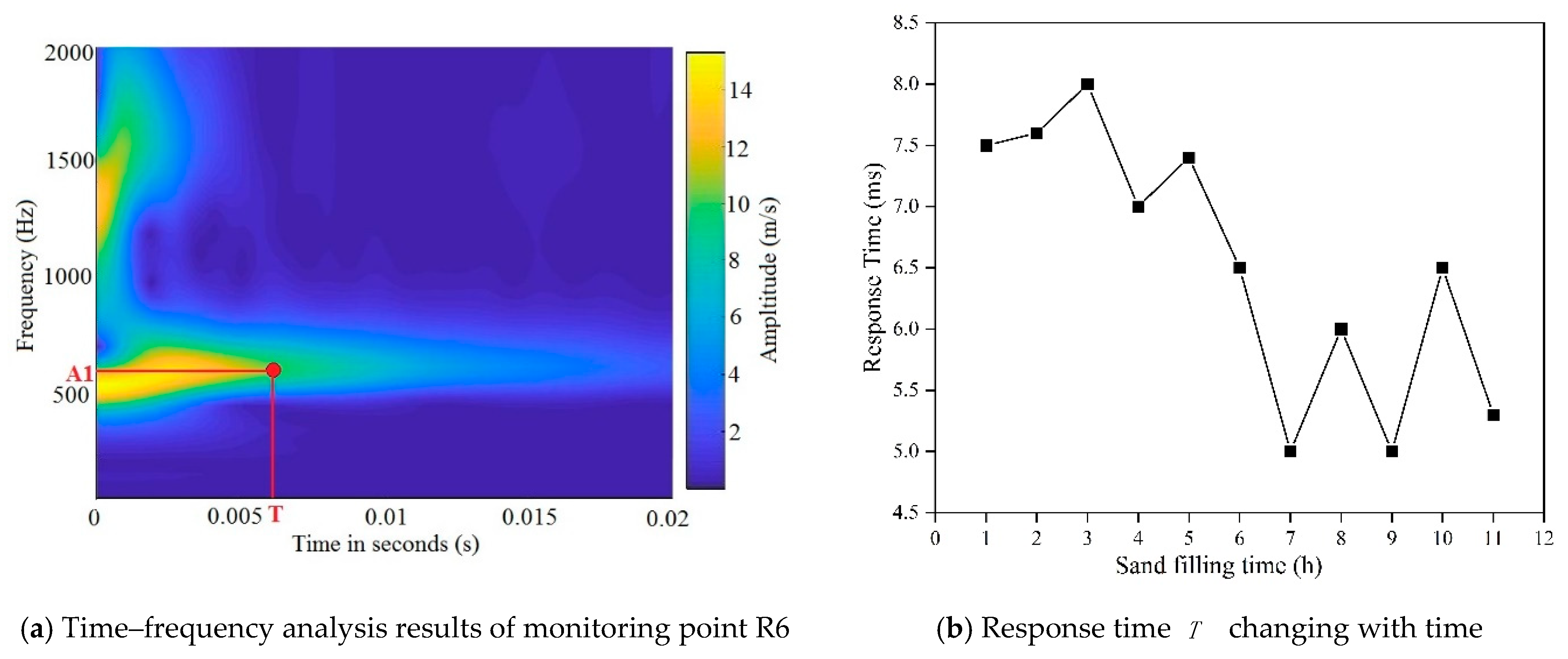
Time-frequency analysis

As the sand-filling progresses, the inside of the medium changes, causing the energy of the elastic wave to change. When the sand-filling process has not started, the material properties inside the medium vary greatly, the wave impedance varies greatly, and elastic waves are reflected multiple times inside. After the sand-filling is completed, the internal wave impedance difference becomes smaller, causing the elastic wave energy to attenuate faster. For time–frequency analysis of the response waveform through the continuous wavelet transform, the calculation formula is

$$W{T}_x(\alpha ,\tau )=\frac{1}{\sqrt{\alpha }}{\displaystyle \int x(t)}{\phi }^{*}(\frac{t-\tau }{\alpha })dt$$

(2)

where $\frac{1}{\sqrt{\alpha }}{\phi }^{*}(\frac{t-\tau }{\alpha })$ is the function obtained by the basic wavelet $\phi (t)$ through displacement $\tau$ and scaling $\alpha$, $x(t)$ is a square-integrable function $(x(t)\in L^2(R))$, and $\tau$ and $\alpha$ are continuous variables. This is the continuous wavelet transform.

By analyzing the attenuation information of the waveform in the time–frequency domain, the state information of the sand deposit can be inferred. Response time $T$, the decay time of the predominant frequency was selected as one of the feature parameters.

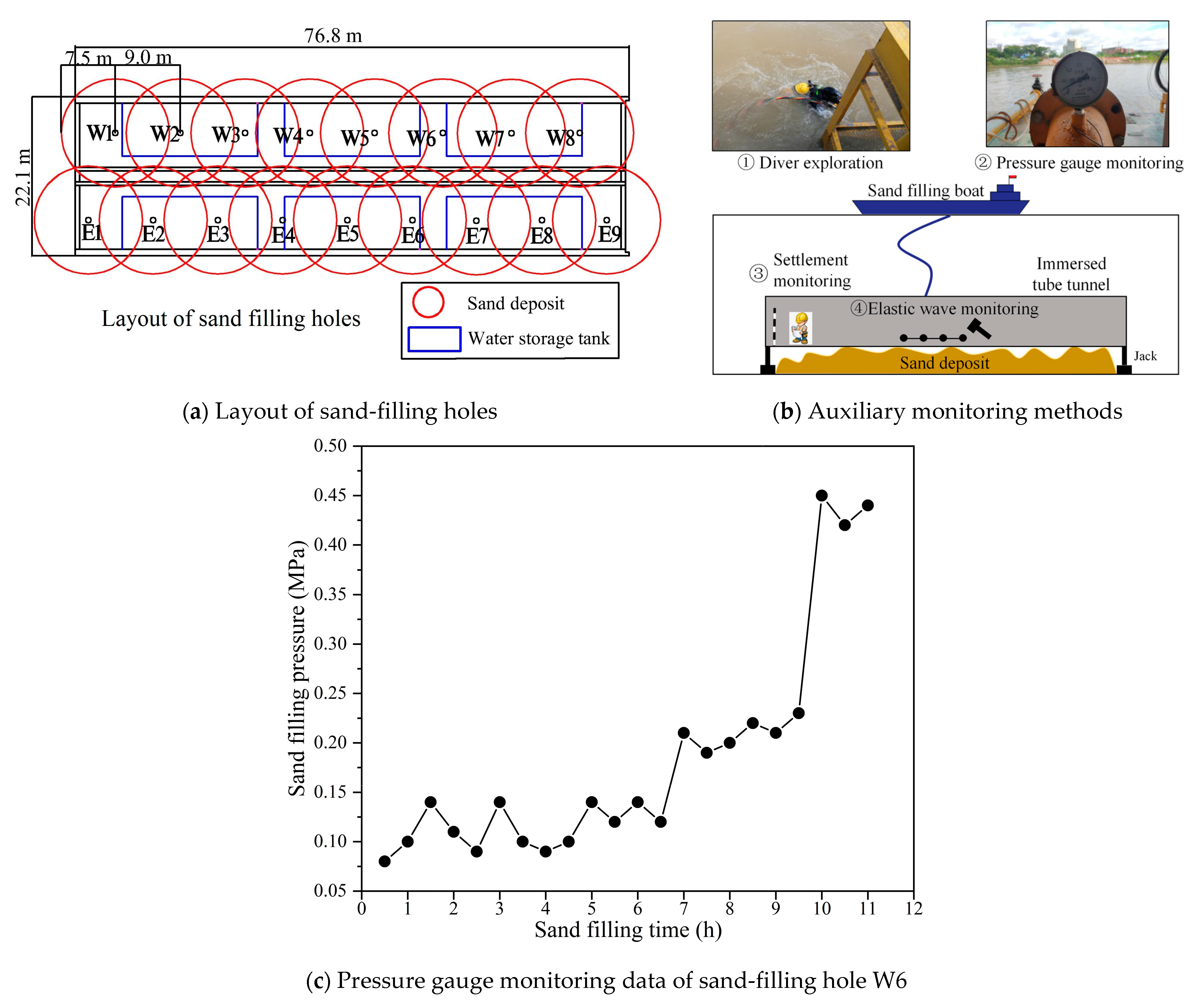
2.2. Sand-Filling Project of Immersed Tube Tunnel Foundation

• Case study: Jinguangdong immersed tube tunnel

The Jinguangdong immersed tube tunnel in Guangzhou, China, was selected as the research object. The foundation of the Jinguangdong immersed tube tunnel was constructed using the sand-filling method. The tunnel is located at 23°2′10″ N, 113°24′30″ E, crossing the Pearl River, with a buried depth of approximately 11 m underwater, as shown in Figure 2. The total length of the tunnel is 460 m, with six pipe sections, and the length of each section is approximately 75–77 m. The size of the cross-section was 8.55 m × 22.1 m. The construction sequence was ordered P6, P5, P1, P2, P3, and P4.

2.

Monitoring the cushion filling effect

The sand-filling effect of the sand deposit corresponding to each sand-filling hole is defined as the cushion filling effect. As shown in Figure 3a, each pipe section was equipped with 17 sand-filling holes, and the distance between neighbouring sand-filling holes was 9 m. The sand-filling process started to fill the side holes (W1, W8, E1, and E9) and ended by filling the middle holes of the pipe section. The designed sand-deposit diffusion radius R_d of each sand-filling hole was 7.5 m. Levelling and rock filling of the river bottom foundation were carried out before sand-filling. The water–sand mix ratio of the filling sand was controlled at 7:1 to 9:1.

Auxiliary monitoring methods, such as the quantity of sand-filling, settlement and lifting, and pressure of sand-filling, were adopted to ensure the quality of the sand foundation, as shown in Figure 3b. Sand-filling quantity monitoring determines the sand-filling process by recording the volume of the poured sand. Settlement and uplift monitoring measures the settlement and uplift of the pipe section through a level gauge. Generally, in the process of sand-filling, the filling or blockage of the hole would result in the sharp rise of the pressure gauge. The pressure gauge monitor judges the state of sand-filling based on the recorded pressure. As is shown in Figure 3c, at 10th hour, the sand-filling pressure suddenly increases, reflecting the completion of sand-filling. All the above indirect methods provide references for the training of the elastic wave monitoring model. The pressure gauge data, uplift state, and sand-filling volume record during the sand-filling process of the P6 pipe section are listed in

Table 1. Data record of the P6 pipe section.

Sand-Filling Hole	Sand-Filling Time (h)	Pipe Section Lifting State
W8	13	Not uplifted
W7	7	Not uplifted
W6	11	Not uplifted
W5	8	Not uplifted
W4	6	The pipe was lifted by 4 cm at the 12th hour
W3	11	Not uplifted
W2	12	Not uplifted
W1	12	Not uplifted
E9	13	Not uplifted
E8	8	Not uplifted
E7	11	Not uplifted
E6	7	Not uplifted
E5	12	Not uplifted
E4	13	Not uplifted
E3	12	The pipe was lifted by 4 cm at the 10th hour

.

2.3. Elastic Wave Monitoring

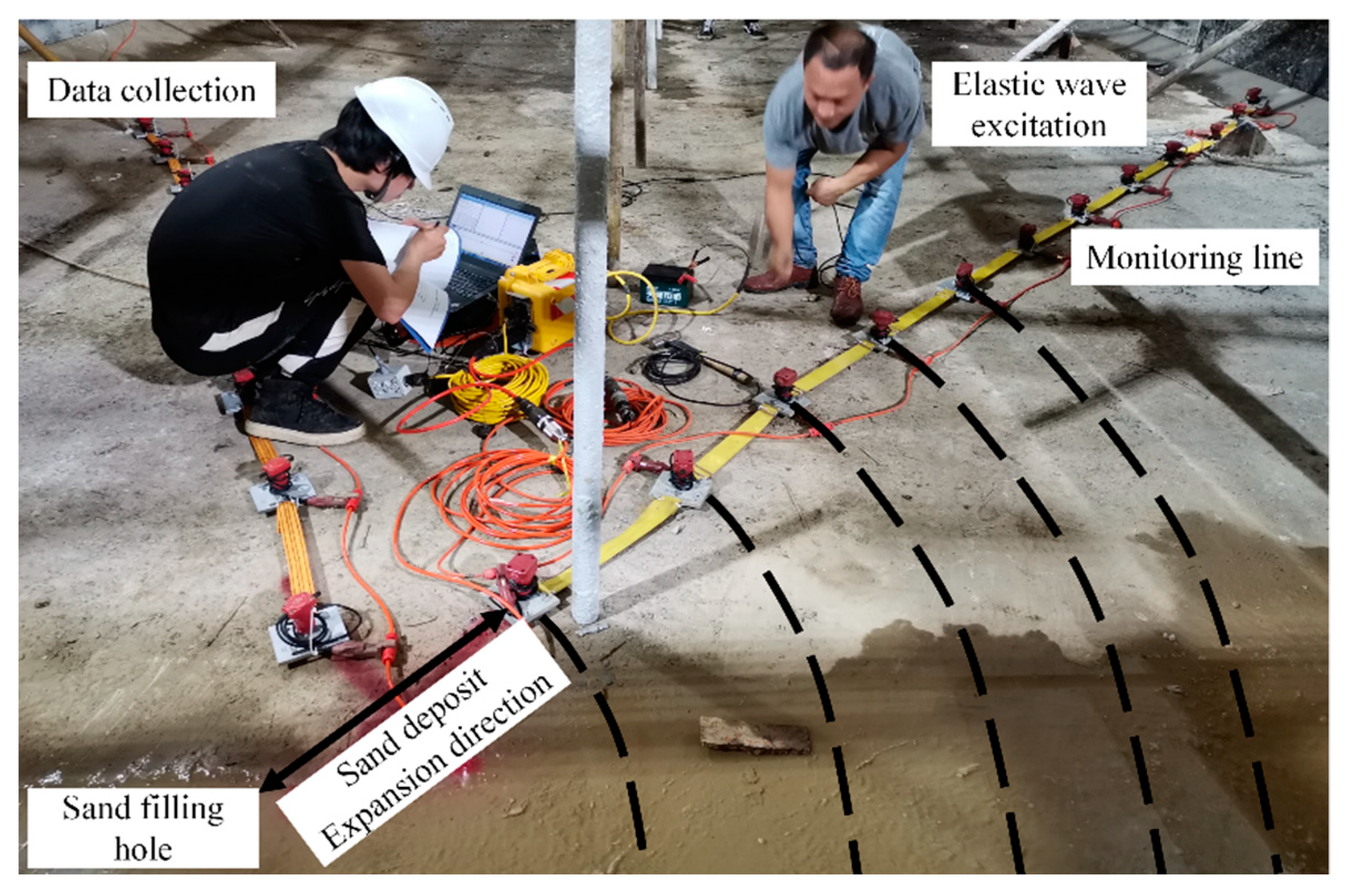
2.3.1. Elastic Wave Monitoring System

The elastic wave monitoring system consists of a detector and coupling device, connection line, power cord, excitation device, excitation hammer, computer, power supply device, etc. A 24-channel Geode digital seismograph was used as the data acquisition equipment, connected to 24-channel single-component detectors. The frequency of the detector was 100 Hz. A 300-g hammer was used as the elastic wave exciter. There were 24 detectors, and the spacing between detectors was 50 cm. The detector used could measure vertical vibration velocity. The data collection method of one excitation and one reception was adopted. The specific parameters of the monitoring system are listed in

Table 2. Device parameters.

Part	Parameters
Geode seismograph	Recording channel: 24 channels Analogue-to-digital conversion: 24 bit Minimum sampling interval: 0.02 ms Low cutoff frequency: 10 Hz Manufacturer: Geode, USA
Detector and coupling device	Moving coil-type velocity detector Natural frequency: 100 Hz Manufacturer: China Chongqing Geological Instrument Factory
Computer	Installed with self-developed data acquisition software
Excitation hammer	Weight: 300 g
Power supply device	DC power supply: 24 V
Connection lines	Long enough

.

To obtain the elastic wave at receiving point R_i, a hammer was used to excite at the impact point I_i. At the same time, the trigger activated the waveform signal record system, and the response waveform of the sand-filling model was recorded and saved. Afterwards, the knocking point of the hammer was moved to the next receiving point to record the response waveform. The data record of a line containing 24 detectors was completed by analogy. In this way, the obtained waveform was saved, and the data acquisition was accomplished.

The process of data acquisition is shown in Figure 4. The sand-filling process usually takes about 10 h empirically based on the designed sand-filling volume and sand-filling speed. Therefore, the monitoring frequency was taken as 1 h. The length of sampling time was determined according to the thickness of propagation medium and wave velocity. The collected wave data had decayed at the time of 0.1 s. Therefore, the sampling time was set to 0.1 s. The uplift state of the pipe section was recorded along with the measurement results of the level gauge, including the cushion filling state, in detail.

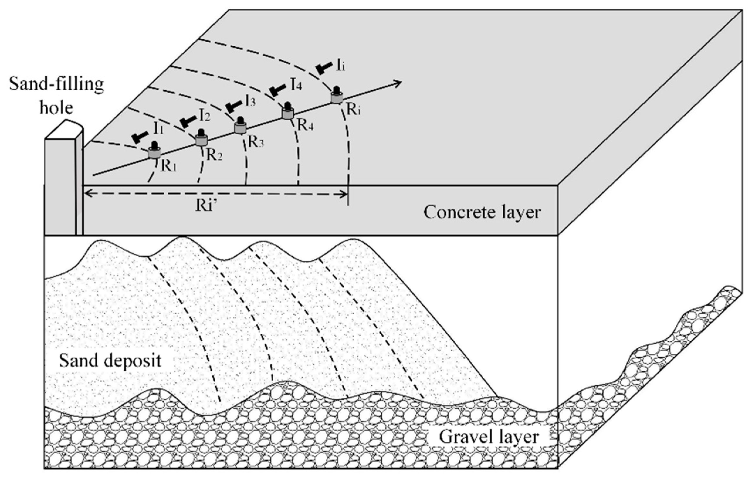
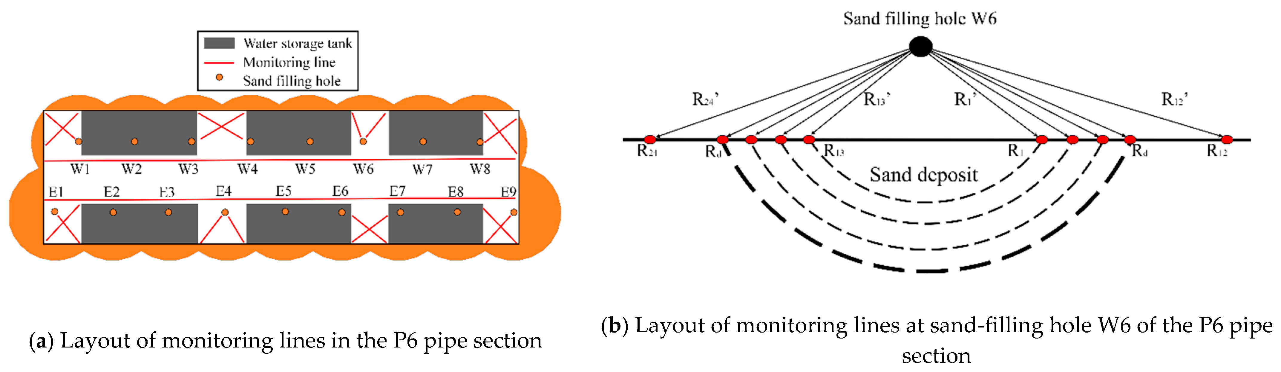
2.3.2. Monitoring Line

Water tanks for controlling the sinking were arranged inside the pipe section, and the water tank was filled with water for weight control during the pipe section sinking process. After the foundation sand was poured, the water tank was removed, and an equal-weight concrete pavement layer would be poured. The monitoring space was limited because of the existence of the water tank. The layout of the monitoring lines was arranged on the radius of the grouting hole, considering the designed radius R_d as the key control parameter. The monitoring lines were maintained during the monitoring process to ensure a stable coupling state. The layout of monitoring lines in P6 pipe section is shown in Figure 5a. The layout of monitoring lines at sand-filling hole W6 is shown in Figure 5b. Two measuring lines were arranged, one at each end of the sand-filling hole, each of which was consisted of 12 detectors, 8 within the designed diffusion radius R_d and 4 outside, aiming to determine the time when the diffusion radius of sand deposit reaches the design diffusion radius R_d.

3. Evaluation Model of Foundation Cushion Filling Effect Based on Elastic Wave Monitoring

3.1. Monitoring Data Analysis

Taking monitoring point R6 of sand-filled hole W6 as an example, the collected elastic wave data were analyzed in the time, frequency, and time–frequency domains.

The waveforms of the monitoring point R6 of the sand-filled hole W6 changing with time are shown in Figure 6a. The attenuation of the elastic wave was completed within 0.03 s, and the attenuation characteristics of the elastic wave were not obvious during sand-filling. Analyzing the waveform reveals that the attenuation of the elastic wave can be divided into three stages: 0–0.005 s is the main response time of the elastic wave, 0.005–0.015 s is the elastic wave attenuation time, and, during 0.015–0.03 s, the elastic wave is basically attenuated. Therefore, the feature parameters, $P{P}_1$, $P{P}_2$, and $P{P}_3$ are defined as follows:

$$\begin{array}{c}P{P}_1=\frac{{\displaystyle {\int }_0^{0.005}\left|f(t)\right|dt}}{\underset{0<t<0.1}{\max }f{(t)}^2},\\ P{P}_2=\frac{{\displaystyle {\int }_{0.005}^{0.015}\left|f(t)\right|dt}}{\underset{0<t<0.1}{\max }f{(t)}^2},\\ P{P}_3=\frac{{\displaystyle {\int }_{0.015}^{0.03}\left|f(t)\right|dt}}{\underset{0<t<0.1}{\max }f{(t)}^2},\end{array}$$

(3)

In Figure 6b, $P{P}_1$, $P{P}_2$, and $P{P}_3$ changing with time are shown. There is a downward trend for $P{P}_1$ with sand-filling time, but it is dynamic. Both $P{P}_2$ and $P{P}_3$ have small changes with sand-filling time.

The results of the spectrum analysis of the monitoring point R6 of sand-filling hole W6 during the sand-filling process are shown in Figure 7. The spectrum of the received elastic wave had two predominant peaks. The frequency and amplitude corresponding to the frequency peaks varied with the sand-filling process. Therefore, the spectrum characteristic parameters $F_1$ (primary frequency), $F_2$ (secondary frequency), $A_1$ (primary frequency amplitude), and $A_2$ (secondary frequency amplitude) were extracted as feature parameters reflecting the waveform. As shown in Figure 7b, $A_1$ reduced significantly with the sand-filling processing. With the formation of the sand deposit, the lower part of the bottom concrete layer changes from water and soil mixture to denser sand deposit. The wave impedance between the two layers (the sand deposit layer and the concrete tunnel layer) decreases, and the energy propagation characteristics change. More energy is transmitted, resulting in a decrease in the reflected elastic wave energy. $F_1$ and $F_2$ are the primary frequency and the secondary frequency, related to the change of the propagation medium of the elastic wave. Since the diffusion of the sand deposit is a dynamic process, $F_1$ and $F_2$ show dynamic characteristic.

The waveform time–frequency analysis results of the monitoring point R6 of sand-filling hole W6 are shown in Figure 8. In the time–frequency domain, the parameter $T$ is defined as the characteristic parameter reflecting the characteristics of the elastic wave in the time–frequency domain. As shown in Figure 8b, the response time T decreases overall with the sand-filling processing, but it is also dynamic.

The feature parameters $P{P}_1$, $P{P}_2$, $P{P}_3$, $F_1$, $F_2$, $A_1$, $A_2$ and $T$ of the elastic wave response waveform were analyzed. With the bottom of the plate filling, the wave impedance at the interface of the bottom plate is correspondingly smaller when it is installed. Therefore, the response waveform amplitude, spectral energy, and reverberation time value of the response waveform measured at the same measuring point after sand-filling are also correspondingly smaller. However, because of the complex construction environment, and because the sand-filling process is affected by many factors, the feature parameters show obvious characteristics of nonlinearity and randomness.

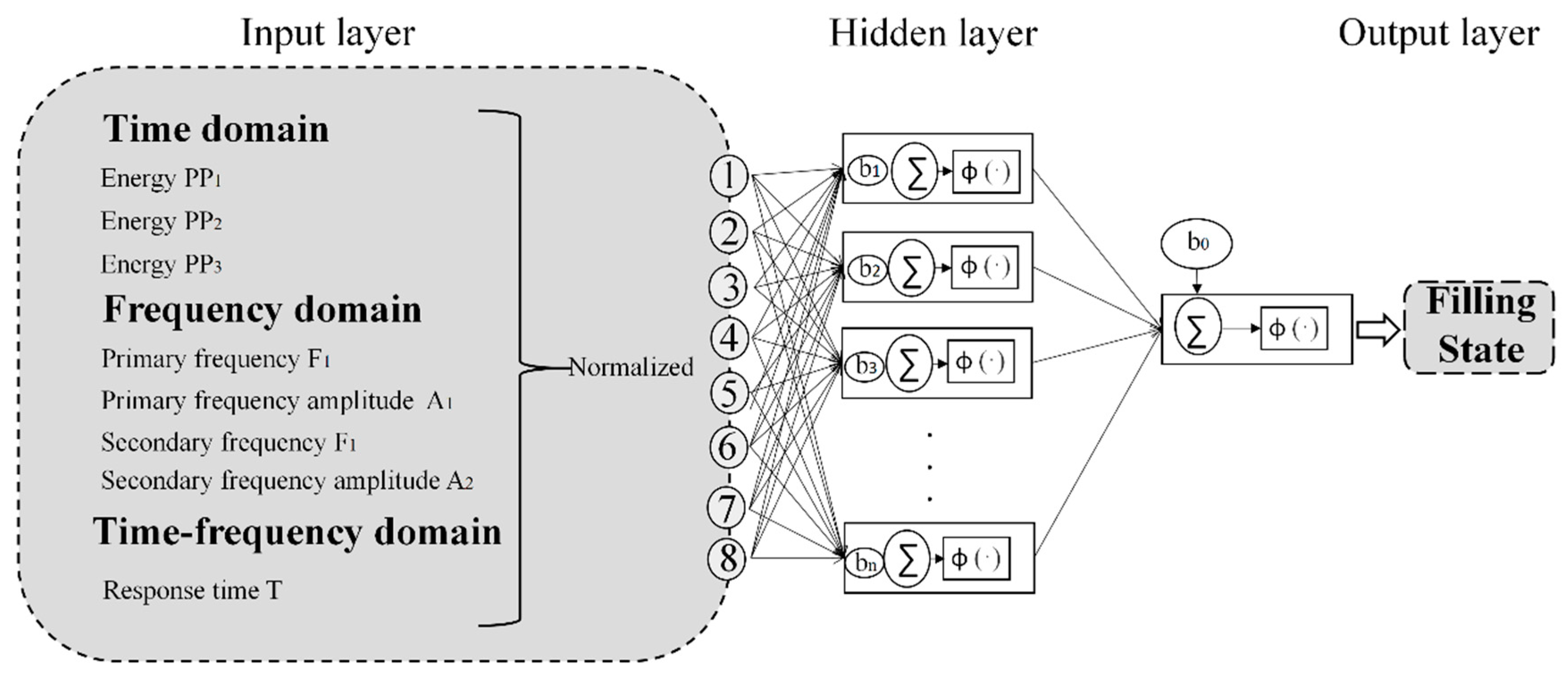
3.2. Elastic Wave Monitoring: BP Neural Network

3.2.1. BP Neural Network Method

A BP neural network is a multilayer feedforward network trained by an error BP algorithm. To establish the relationship between the elastic wave data and the state of the sand deposit, a neural network evaluation model was constructed. The input layer contained the characteristic parameters of the collected elastic wave: $P{P}_1$, $P{P}_2$, $P{P}_3$, $F_1$, $F_2$, $A_1$, $A_2$ and $T$. The output layer is the two states corresponding to the monitoring points. The hidden layer is the “hub” connecting the input and output of the neural network. At present, there is no fixed theoretical basis for the choice of the hidden layer. Through repeated practice, the hidden layer is selected as three layers, and the numbers of nodes are 15, 20, and 10.

Based on the above analysis, the BP neural network structure of the sand-filling state of the immersed tube tunnel was established. A graphical representation of the architecture of the proposed system is shown in Figure 9. The output of each processing node is connected to each processing unit in the next layer, but the processing units in the same layer do not form a connection.

3.2.2. Sample Selection and Training

The elastic wave data with a clear sand-filling state were selected to train the network model. The data collected each time were classified into two states, as listed in

Table 3. States of monitoring points.

Classification	State
State 1	Not filled
State 2	Filled

, representing whether the sand deposit under the detection point was in contact with the bottom concrete of the immersed tube.

Specifically, for the middle holes, there are two ends: a free and a constrained end. The free end is the one where the adjacent sand-filling hole is unfilled, and the constrained end is the end where the adjacent sand-filling hole is filled. The diffusion of the sand deposit at the free end can be considered a state where the initial diffusion radius is 0 and the finished state diffusion radius reaches R_d. The free end data were filtered out, and the corresponding sand deposit state was determined according to the recorded information. The selection of the training data also considered other field information, such as the information of the pressure gauge on the sand-filling vessel, the resulting feedback of the diver’s exploration, and the uplift of the pipe section shown in Table 1. During the process of sand-filling holes W4 and E3, there was a pipe section uplifting. This was caused by the jacking up of the sand plate. The state of the detection point was state 2. Additional measurements were carried out when the pipe section was raised, and the collected data were defined as state 2. In this way, 1000 sets of data with clear states were selected: 500 sets of data for State 1 and 500 sets of data for State 2.

Before the BP neural network model training, the Z-score normalization method was used to normalize each group of characteristic data to eliminate the influences of dimension and value range difference between indices. The regularization, momentum, and learning rate parameters were set to 0.2, 0.01, and 0.05, respectively. The parameters were tuned accordingly to obtain optimal performance. The number of hidden layers is set to 3, the numbers of nodes of which are 15, 20 and 10. The tan-sigmoid function was selected as the transfer function. Levenberg-Marquardt algorithm was adopted for the fastest convergence speed for medium-scale BP neural networks. The goal error of the training set was set as 0.001. When the error of the training set during the iteration was less than 0.001, the training process stopped. The error function gradually decreased with an increase in the number of iterations, reaching 0.00099588 at 321 iterations, showing that the neural network was convergent.

After training, the training set data were input into the trained model for simulation, and the difference between the simulation result and its true value was defined as the error. The error change of the model on the training set is shown in Figure 10. The errors of 800 training datasets were all within 0.01, indicating that the error was small.

3.2.3. Test for BP Neural Network

To test the accuracy of the model, 100 groups of data with clear states and not involved in the training were randomly selected. The testing results are shown in Figure 11. Among the 100 groups of test samples, the state was successfully evaluated for 93 groups, and seven groups were misjudged. For four groups, the unfilled state was misjudged as full; for three, the full was misjudged as not full. The overall inspection accuracy of this model for the test set was 93%. This indicates that the trained network model effectively evaluated the sand-filling state.

4. Application of Spatiotemporal Monitoring Model

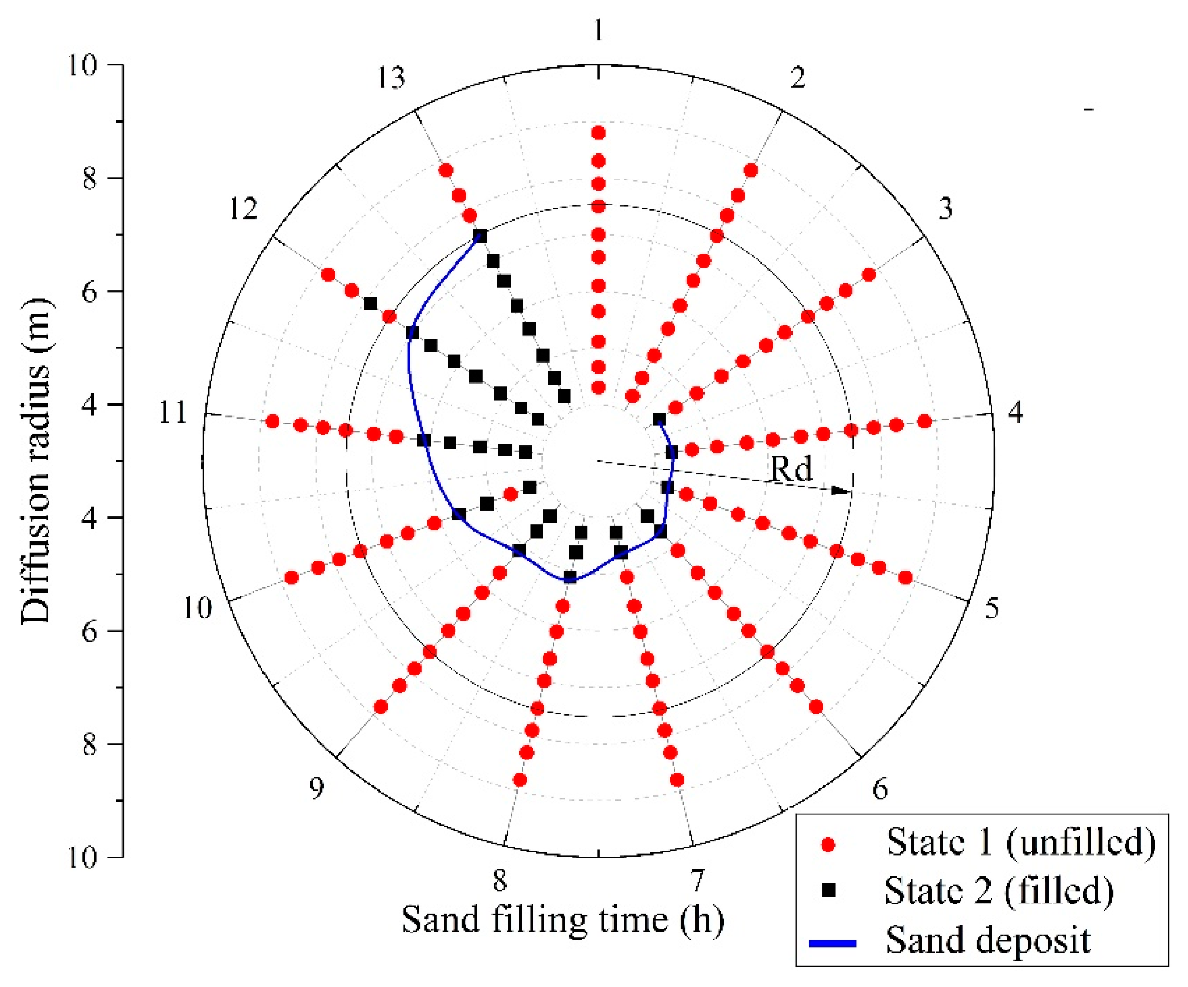
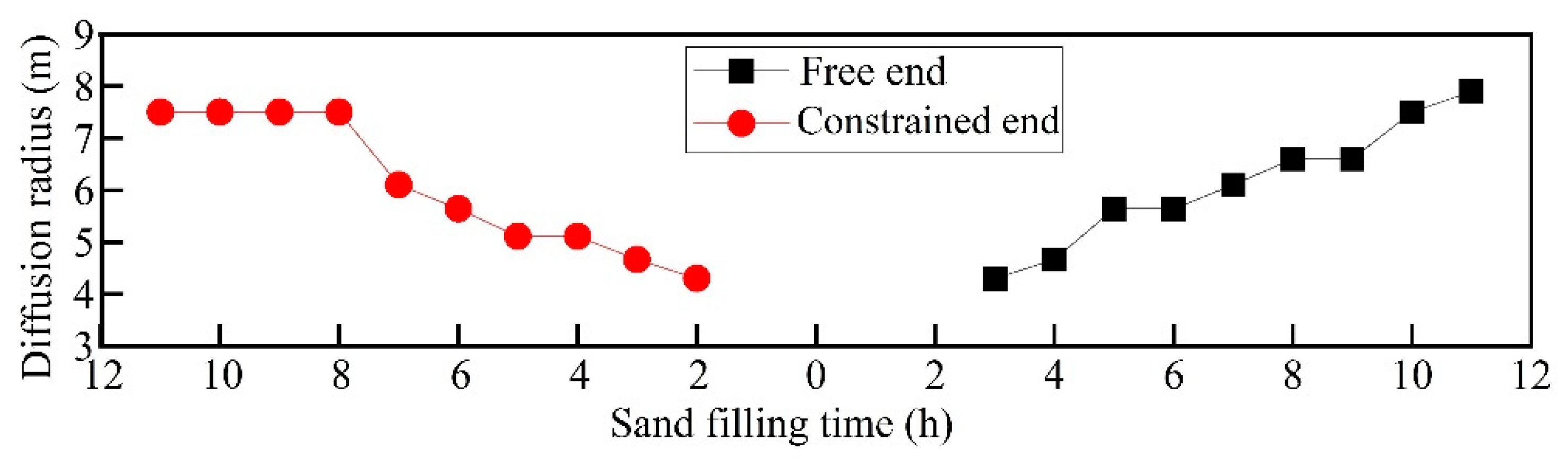
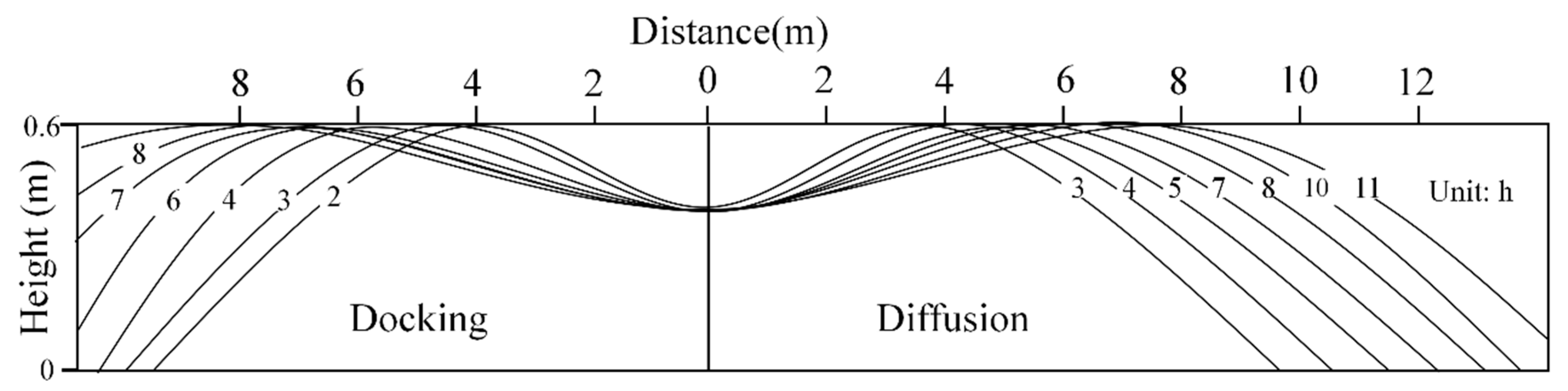
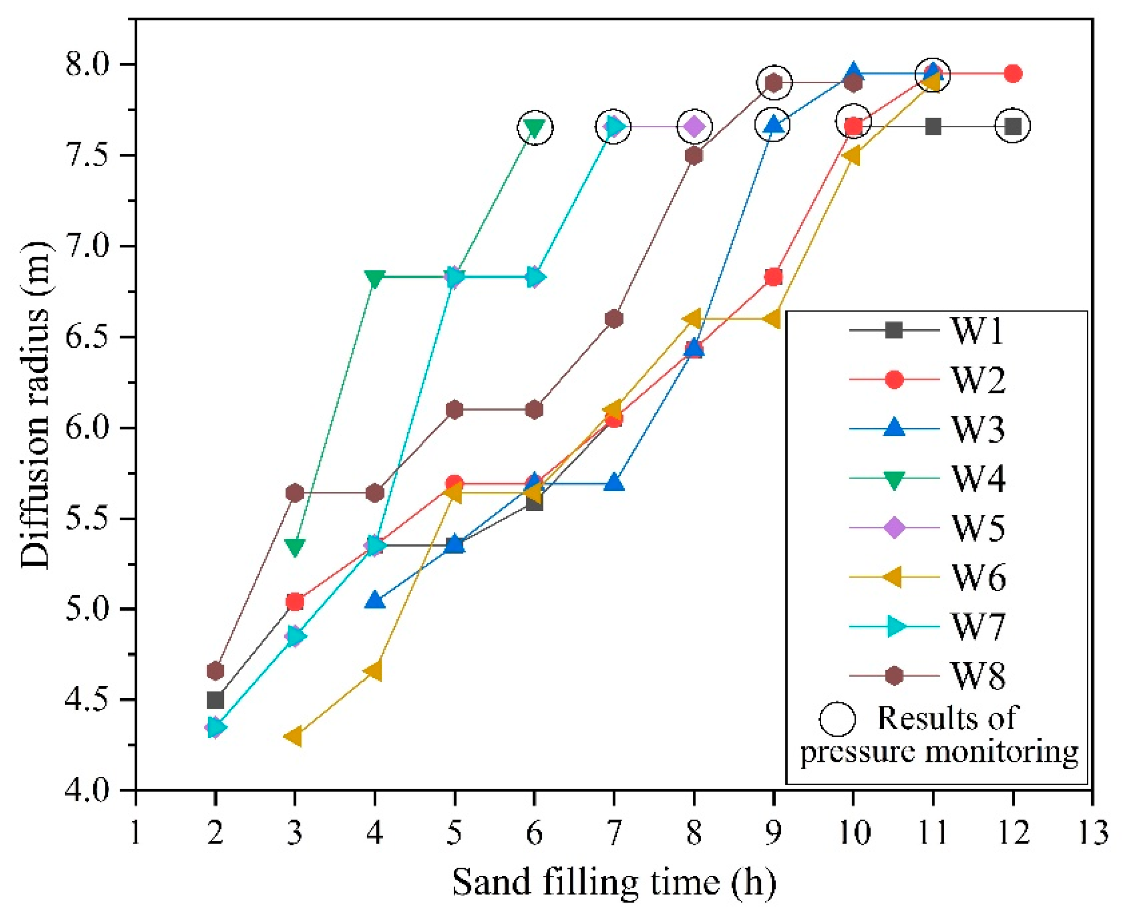
4.1. Spatiotemporal Monitoring for Sand-Filling

To realize the spatiotemporal monitoring of the state of the sand deposit, the sand-filling holes were divided into two types: side and middle holes. A side hole is a hole at the edge of the pipe section, where both ends of the sand deposit are free boundaries. A middle hole is a hole in the middle of the pipe section. The sand deposit of middle holes have one free boundary and the constrained boundary is affected by the adjacent sand deposit.

For the side holes, the formation mechanism of the sand deposit is that the sand gradually accumulates along the direction of the diffusion radius. As shown in Figure 12, for the sand-filled hole W8, elastic wave data collection was performed every hour, and the sand-filling state was predicted by the trained neural network model. With the progress of sand-filling, along the direction of the diffusion radius, the state of each monitoring point gradually changed from the unfilled state to the filled state, and the sand deposit gradually formed. At the 13th hour, the diffusion radius reached design diffusion radius R_d.

For the middle holes, monitoring lines were arranged on both the constrained boundary and the free boundary. The diffusion mechanism on both boundaries of the sand-filling hole takes different forms. As shown in Figure 13a, for the free boundary, it can be found that the state of the monitoring points within the diffusion radius gradually changes from state 1 (unfilled) to state 2 (filled) with the progress of sand-filling, indicating the expansion of the sand deposit. The speed of sand deposit formation is low at first, and then it is gradually accelerated. Finally, the diffusion radius reached R_d at the 11th hour. However, for the constrained boundary, the speed of sand deposit formation is much higher than that at the free boundary. The formation mechanism at the constrained boundary is obviously different from that at the free boundary. The state of several monitoring points outside the diffusion radius is in the state 2 because of the sand spreading during the previous sand-filling process at adjacent holes. Therefore, for different categories of boundaries at the sand-filling hole, the formation mechanism of sand deposits could exhibit different forms. At the free boundary, the formation of sand deposits is accompanied by the diffusion and accumulation of filling sand, like the sand-filling hole W8 in Figure 12. At the constrained boundary, under the influence of adjacent sand-filling holes, there are partially filled sand deposits or unfilled sand within the diffusion radius. The sand-filling process at the constrained boundary requires less filling time and exhibits the docking form of the sand deposit formation.

According to the obtained spatiotemporal model of sand-filling hole W6, the change in the sand-deposit diffusion radius of sand-filling hole W6 over time can be evaluated. For each sand-filling time, the distance between the sand-filling hole and the monitoring point, which is in state 2 and closest to the sand-filling hole, is considered as the diffusion radius at that moment. As the sand-filling progresses, the relationship between the diffusion radius and sand-filling time can be obtained. When the diffusion radius reaches the design value R_d, the sand-filling process can be stopped. The diffusion radius with the time of sand-filling hole W6 is shown in Figure 14. At the free end, the sand deposit required a long sand-filling time, and it was gradually filled at the 11th hour. At the constrained end, the sand deposit was well connected to the adjacent sand deposit at the 8th hour, and the connection was stable. Since the adjacent sand deposits have been formed, the amount of sand required on the constrained end is less than that of the free end. Therefore, the constrained end of the sand deposit can be filled in a shorter time. On the contrary, for the free end, since the sand deposit is not constrained by the adjacent sand deposit, the sand-filling time is longer.

According to the diffusion radius with sand-filling time, the diffusion model of the expansion of the sand-filling hole W6 is shown in Figure 15. For the free end, the sand deposit gradually expands along the direction of the diffusion radius, which is defined as diffusion form. For the constrained end, the sand deposit is formed faster and connected with the adjacent sand deposit, which is defined as docking form. With the help of the monitoring and evaluation model, the state of the sand deposit was well monitored, providing guidance for sand-filling construction.

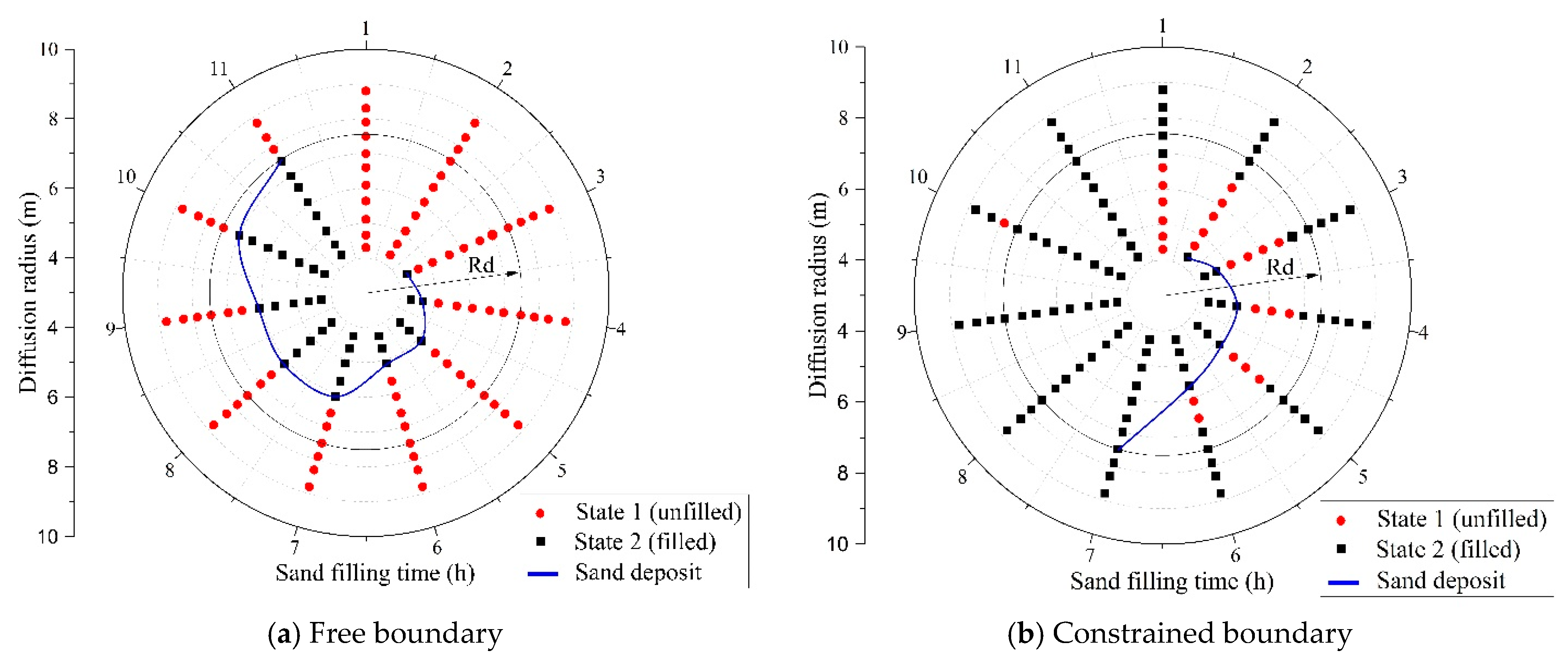
4.2. Monitoring Evaluation for Cushion Filling Results of P5 Pipe Section

The evaluation results for the P5 pipe section from the trained neural network and the relationship between the diffusion radius of each sand-filling hole and time are shown in Figure 16. For the entire P5 pipe section, the sand-filling time required for side holes is longer, such as 12 h for sand-filling holes W1 and W2. The sand-filling time required for middle holes is shorter, such as 6 h for sand-filling hole W4. Whether it is a side hole or a middle hole, this model reflects the relationship between the diffusion radius and sand-filling time well. When the results of pressure gauge monitoring are compared with this model, the results of elastic wave monitoring are in good agreement with the pressure gauge values. The black circle in Figure 16 indicates the time when the pressure gauge suddenly increases for each sand-filling hole. It can be seen that the time when the pressure gauge suddenly increases shows a consistent trend with the results of spatiotemporal monitoring. The proposed model can evaluate the diffusion radius of the sand deposit very well, achieving the effect of time and space monitoring of sand-filling construction of immersed tunnels.

Due to the proposed neural network model, the construction process of the P5 pipe section was smooth, and there were no abnormal phenomena, such as sand-filling hole plugging or uneven pipe section uplift. Moreover, the consecutive settlement of the pipe section was small (4 cm for six months), satisfying the design requirements and confirming the applicability of this method. Therefore, this model can provide guidance and real-time monitoring for construction.

For researches on the sand-filling of immersed tube tunnels, model tests under different conditions were carried out to explore the law of sand deposit expansion [10]. In the study of the evaluation for the sand deposit state during construction, the P-wave impact imaging method was proposed to detect the radius and the distribution of relative compactness of sand deposits [12]. The sand deposits in both model testing and field monitoring are assumed to be with a free boundary. In the present study, a spatiotemporal monitoring method is proposed to evaluate the state of the sand deposit, and the influence of boundary conditions on the expansion of the sand deposit for different types of holes (side holes, middle holes) is analysed. Regarding the diffusion law of the sand deposit with free boundary, the analysis results of this paper show a high consistency with the related literature.

5. Conclusions

A spatiotemporal monitoring and evaluation method was proposed based on the elastic wave testing method and the BP neural network model.

• By analyzing the elastic wave data in the time, frequency, and time–frequency domains, it was possible to determine the feature parameters $P{P}_1$, $P{P}_2$, $P{P}_3$, $F_1$, $F_2$, $A_1$, $A_2$ and $T$ to characterize the elastic wave. The feature parameters of elastic wave data change with the sand-filling process and exhibit nonlinearity and strong randomness.
• Using a neural network model, the mapping relationship between the collected elastic wave data and the sand-filling state was established to evaluate the sand-filling state. The accuracy of the proposed model for the test set was 93%.
• The side holes and middle holes were classified and examined to analyze the diffusion characteristics of the sand deposit. For sand-filling hole W8, the proposed model effectively reflected the sand-filling state. The model could monitor the state of the sand deposit during the sand-filling construction process through the elastic wave monitoring results to provide knowledge about the sand-filling construction.

The proposed method provides a new perspective in the monitoring of the immersed tube tunnel foundation cushion filling effect. This is essential for the safety and quality of the immersed tube tunnel. Although this study focused on the immersed tube tunnel, the method can also be applied to other areas of sand-filling or grouting monitoring.

References

1. Wei, G.; Qiu, H. Summary of model tests and settlement characteristics of base layer in immersed tube tunnel. Appl. Mech. Mater. 2013, 2574, 1421–1425. [Google Scholar] [CrossRef]
2. Glerum, A. Developments in immersed tunneling in Holland. Tunn. Undergr. Space Technol. 1995, 10, 455–462. [Google Scholar] [CrossRef]
3. Norman, D. The DEAS tunnel. Soc. Am. Mil. Eng. 1959, 342, 289–292. [Google Scholar]
4. Stingl, V.; Eidelsburger, S.; Fruehauf, J.; Hangebrock, D. Jin Shazhou tunnel on the high-speed railway line Wuhan-Guangzhou- one of the most challenging tunnel constructions in China. Bauingenieur 2010, 85, 105–111. [Google Scholar]
5. Grantz, W. Immersed tunnel settlements—Part 2: Case histories. Tunn. Undergr. Space Technol. 2001, 16, 203–210. [Google Scholar] [CrossRef]
6. Wei, G.; Su, Q. Application of three-parameter model in settlement calculation of immersed tube tunnel. Appl. Mech. Mater. 2013, 470, 298–303. [Google Scholar] [CrossRef]
7. Li, Y.; Cui, J.; Mo, H.; Li, W.; Yuan, J. Sand deposit arrangement and construction optimization for large-section immersed tube tunnel foundations via the sand flow method. Soil Mech. Found. Eng. 2017, 54, 324–329. [Google Scholar] [CrossRef]
8. Wang, S.; Zhang, X.; Bai, Y. Comparative study on foundation treatment methods of immersed tunnels in China. Front. Struct. Civ. Eng. 2020, 14, 82–93. [Google Scholar] [CrossRef]
9. Li, B.; Chen, Z.; Liu, Z. Foundation settlement prediction of immersed tunnel based on monitoring data. IOP Conf. Ser. Mater. Sci. Eng. 2020, 780, 072028. [Google Scholar] [CrossRef]
10. Li, W.; Fang, Y.; Mo, H. Model test of immersed tube tunnel foundation treated by sand-flow method. Tunn. Undergr. Space Technol. 2014, 40, 102–108. [Google Scholar] [CrossRef]
11. Weng, X.; Feng, Y.; Lou, Y. The mechanical performance of shear key of immersed tube tunnel with differential foundation settlement. J. Sens. 2015, 2016, 1–9. [Google Scholar] [CrossRef] [Green Version]
12. Liu, Z.; Zhou, C.; Lu, Y.; Yang, X.; Liang, Y.; Zhang, L. Application of FRP Bolts in Monitoring the Internal Force of the Rocks Surrounding a Mine-Shield Tunnel. Sensors 2018, 18, 2763. [Google Scholar] [CrossRef] [PubMed] [Green Version]
13. Che, A.; Zhu, R.; Fan, Y. An impact imaging method for monitoring on construction of immersed tube tunnel foundation treated by sand-filling method. Tunn. Undergr. Space Technol. 2019, 85, 1–11. [Google Scholar] [CrossRef]
14. Cao, R.; Ma, M.; Liang, R.; Niu, C. Detecting the Void behind the Tunnel Lining by Impact-Echo Methods with Different Signal Analysis Approaches. Appl. Sci. 2019, 9, 3280. [Google Scholar] [CrossRef] [Green Version]
15. Chen, Y.; Irfan, M.; Uchimura, T.; Cheng, G.; Nie, W. Elastic wave velocity monitoring as an emerging technique for rainfall-induced landslide prediction. Landslides 2018, 15, 1155–1172. [Google Scholar] [CrossRef]
16. Chroscielewski, J.; Rucka, M.; Wilde, K.; Witkowski, W. Elastic wave propagation in frame structure in the context of structural health monitoring. In Proceedings of the Fourth European Workshop on Structural Health Monitoring, Cracow, Poland, 2–4 July 2008; pp. 467–473. [Google Scholar]
17. Tao, S.; Uchimura, T.; Fukuhara, M.; Tang, J.; Chen, Y.; Huang, D. Evaluation of Soil Moisture and Shear Deformation Based on Compression Wave Velocities in a Shallow Slope Surface Layer. Sensors 2019, 19, 3406. [Google Scholar] [CrossRef] [Green Version]
18. Zak, A.; Radzien’ski, M.; Krawczuk, M.; Ostachowicz, W. Damage detection strategies based on propagation of guided elastic waves. Smart Mater. Struct. 2012, 21, 035024. [Google Scholar] [CrossRef]
19. Zima, B.; Rucka, M. Guided waves for monitoring of plate structures with linear cracks of variable length. Arch. Civ. Mech. Eng. 2016, 16, 387–396. [Google Scholar] [CrossRef]
20. Chaki, S.; Bourse, G. Guided ultrasonic waves for non-destructive monitoring of the stress levels in prestressed steel strands. Ultrasonics 2009, 49, 162–171. [Google Scholar] [CrossRef]
21. Worden, K.; Staszewski, W.; Hensman, J. Natural computing for mechanical systems research: A tutorial overview. Mech. Syst. Signal. Process. 2011, 25, 4–111. [Google Scholar] [CrossRef]
22. Bao, Y.; Chen, Z.; Wei, S. The state-of-art of data science and engineering in structural health monitoring. Engineering 2019, 5, 234–242. [Google Scholar] [CrossRef]
23. Sattari, M.T.; Avram, A.; Apaydin, H.; Matei, O. Soil Temperature Estimation with Meteorological Parameters by Using Tree-Based Hybrid Data Mining Models. Mathematics 2020, 8, 1407. [Google Scholar] [CrossRef]
24. Noori Hoshyar, A.; Rashidi, M.; Liyanapathirana, R.; Samali, B. Algorithm Development for the Non-Destructive Testing of Structural Damage. Appl. Sci. 2019, 9, 2810. [Google Scholar] [CrossRef] [Green Version]
25. Ni, K.; Ramanathan, N.; Chehade, M.; Balzano, L.; Nair, S.; Zahedi, S. Sensor network data fault types. ACM Trans. Sens. Netw. 2009, 5, 29. [Google Scholar] [CrossRef] [Green Version]
26. Luo, Y.; Ye, Z.; Guo, X.; Qiang, X.; Chen, X. Data missing mechanism and missing data real-time processing methods in the construction monitoring of steel structures. Adv. Struct. Eng. 2015, 18, 585–601. [Google Scholar] [CrossRef]
27. Yang, Y.; Nagarajaiah, S. Harnessing data structure for recovery of randomly missing structural vibration responses time history: Sparse representation versus low-rank structure. Mech. Syst. Signal Process. 2016, 74, 165–182. [Google Scholar] [CrossRef]
28. Zhang, Z.; Luo, Y. Restoring method for missing data of spatial structural stress monitoring based on correlation. Mech. Syst. Signal Process. 2017, 91, 266–277. [Google Scholar] [CrossRef]
29. Flood, I. Towards the next generation of artificial neural networks for civil engineering. Adv. Eng. Inf. 2008, 22, 4–14. [Google Scholar] [CrossRef]
30. Hinton, G.; Salakhutdinov, R.R. Reducing the dimensionality of data with neural networks. Science 2006, 313, 504–507. [Google Scholar] [CrossRef] [Green Version]
31. Nazarko, P.; Ziemia’nski, L. Damage detection in aluminum and composite elements using neural networks for Lamb waves signal processing. Eng. Fail. Anal. 2016, 69, 97–107. [Google Scholar] [CrossRef]
32. Samarin, M.; Zweifel, L.; Roth, V.; Alewell, C. Identifying Soil Erosion Processes in Alpine Grasslands on Aerial Imagery with a U-Net Convolutional Neural Network. Remote Sens. 2020, 12, 4149. [Google Scholar] [CrossRef]
33. Beskopylny, A.; Lyapin, A.; Anysz, H.; Meskhi, B.; Veremeenko, A.; Mozgovoy, A. Artificial Neural Networks in Classification of Steel Grades Based on Non-Destructive Tests. Materials 2020, 13, 2445. [Google Scholar] [CrossRef]
34. Nazarko, P. Axial force prediction based on signals of the elastic wave propagation and artificial neural networks. MATEC Web Conf. 2019, 262, 10009. [Google Scholar] [CrossRef]
35. Ratnam, T.; Ghosh, D.; Negash, B. The integration of elastic wave properties and machine learning for the distribution of petrophysical properties in reservoir modeling. IOP Conf. Ser. Mater. Sci. Eng. 2018, 352, 012024. [Google Scholar] [CrossRef]
Figure 1. Elastic wave monitoring method.
Applsci 11 01084 g001
Figure 2. Jinguangdong immersed tube tunnel.
Applsci 11 01084 g002
Figure 3. Foundation cushion filling effect monitoring.
Applsci 11 01084 g003
Figure 4. Data acquisition process.
Applsci 11 01084 g004
Figure 5. Monitoring line.
Applsci 11 01084 g005
Figure 6. Elastic wave data in the time domain.
Applsci 11 01084 g006
Figure 7. Results of the spectrum analysis.
Applsci 11 01084 g007
Figure 8. Time–frequency analysis results.
Applsci 11 01084 g008
Figure 9. BP neural network structure of the sand-filling state.
Applsci 11 01084 g009
Figure 10. Error change of the model.
Applsci 11 01084 g010
Figure 11. Test results of BP neural network.
Applsci 11 01084 g011
Figure 12. Spatiotemporal monitoring results of sand-filling hole W8.
Applsci 11 01084 g012
Figure 13. Spatiotemporal monitoring results of sand-filling hole W6.
Applsci 11 01084 g013
Figure 14. Diffusion radius with the time of sand-filling hole W6.
Applsci 11 01084 g014
Figure 15. Diffusion model of sand-filling hole W6.
Applsci 11 01084 g015
Figure 16. Diffusion radius with time of P5 pipe section.
Applsci 11 01084 g016