
Sources and Metal Pollution of Sediments from a Coastal Area of the Central Western Adriatic Sea (Southern Marche Region, Italy)

 ,
,  ,
,  , , and
Abstract
:1. Introduction
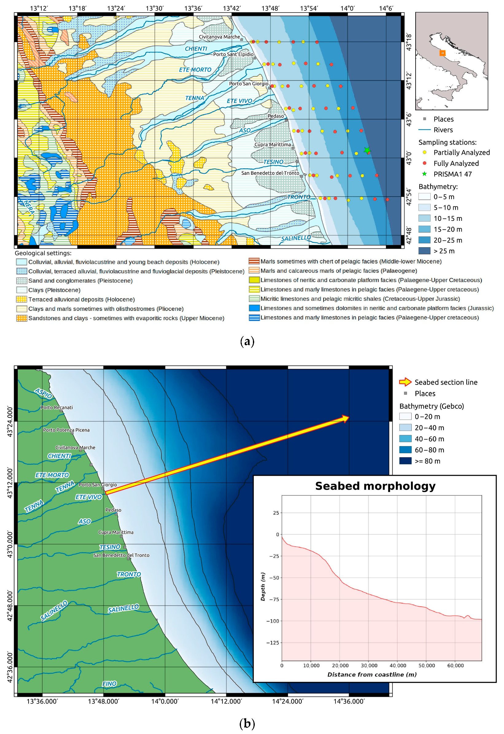
2. Study Area
3. Materials and Methods
3.1. Sampling
3.2. Grain-Size and Organic Geochemistry
3.3. Inorganic Geochemistry
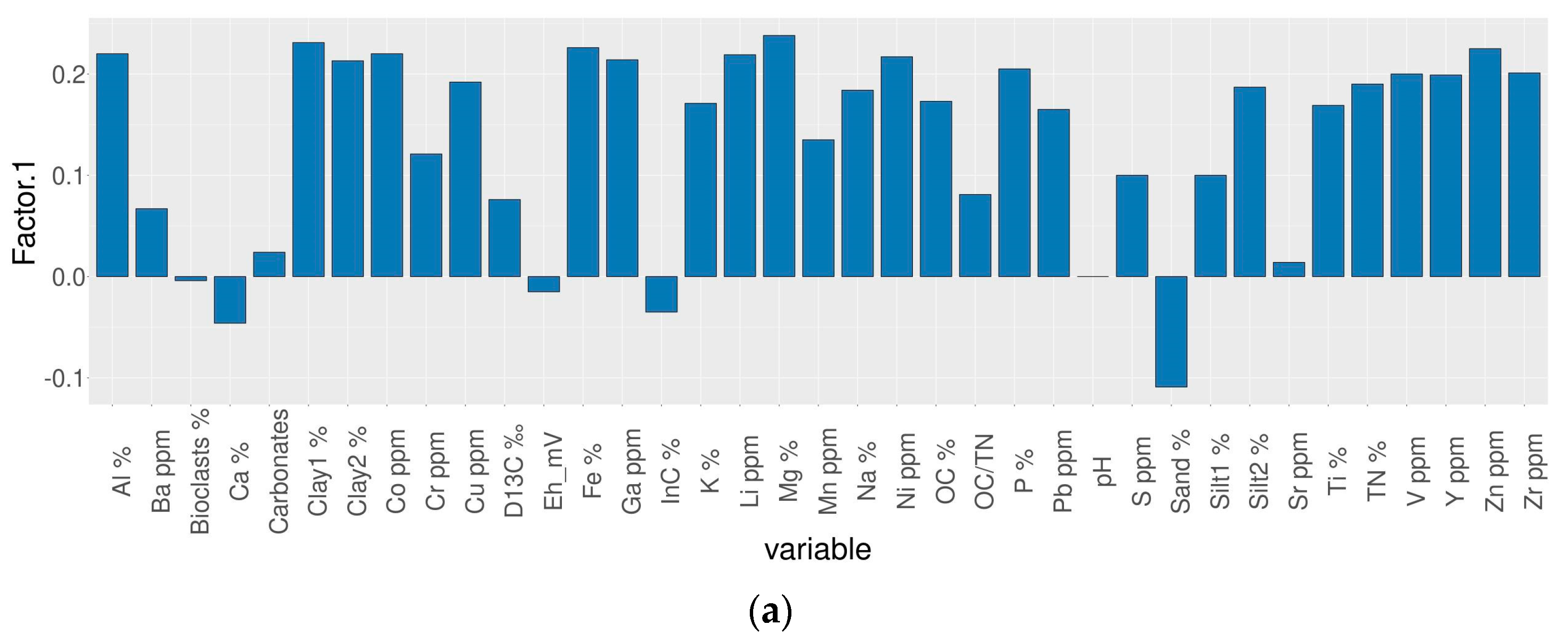
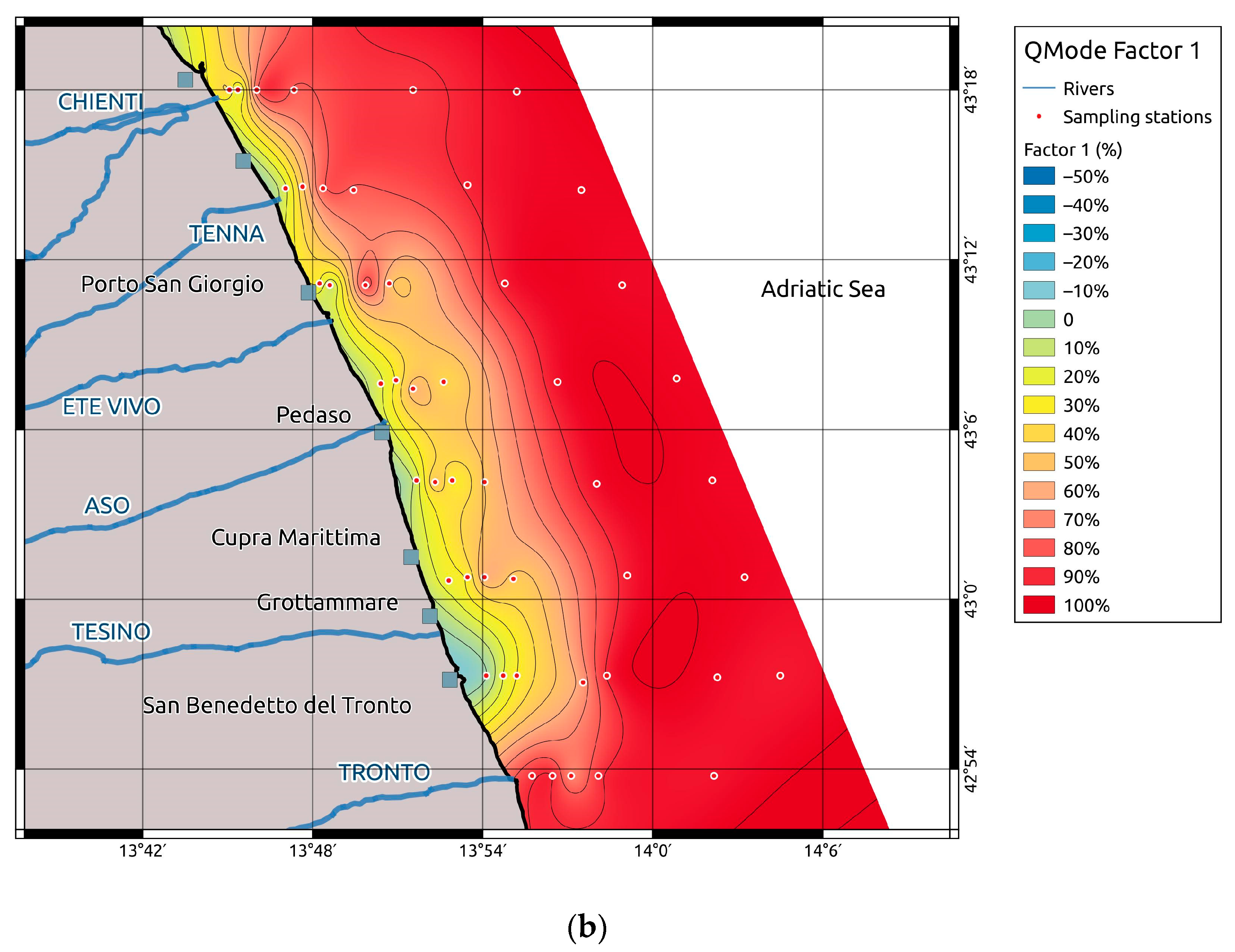
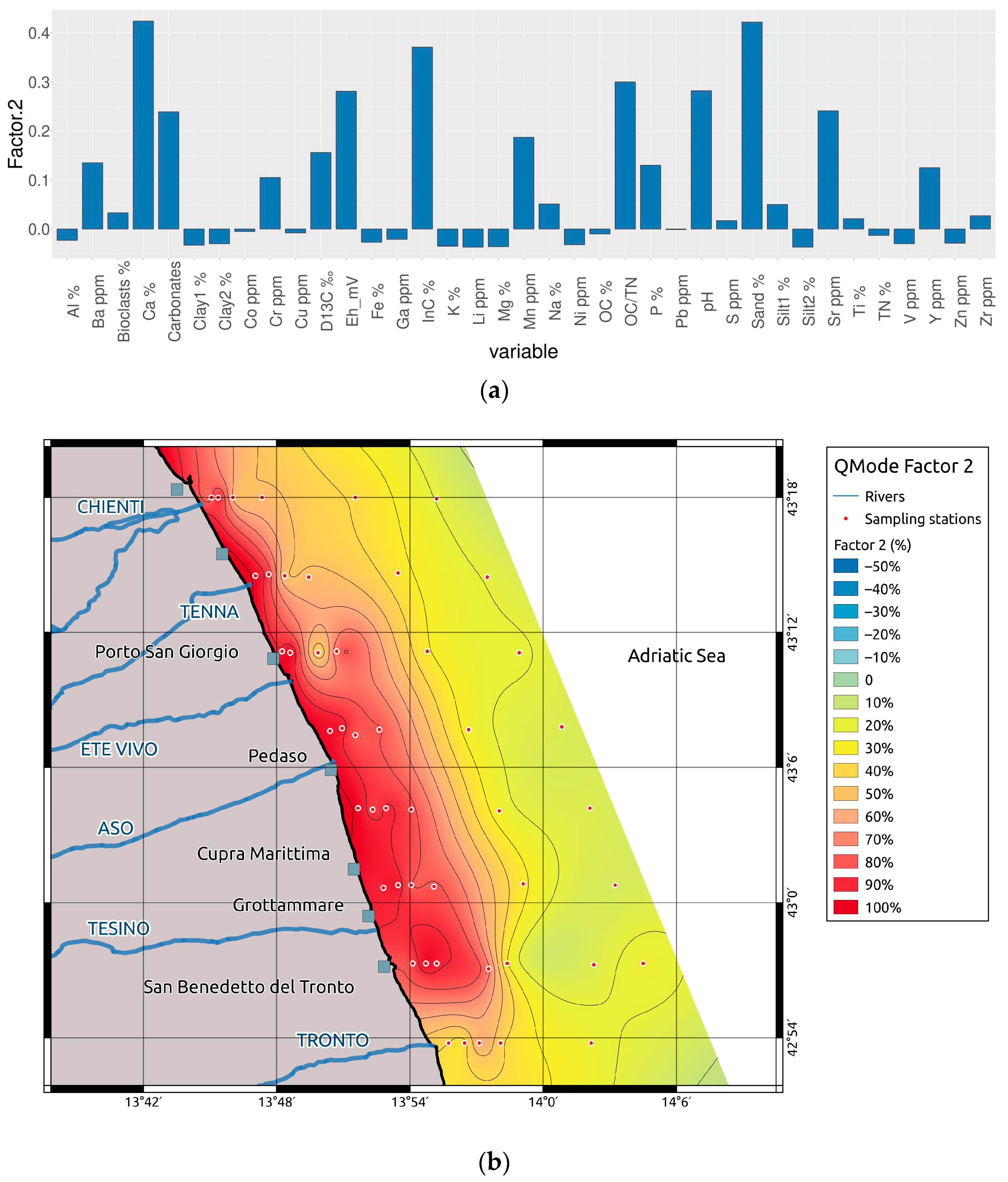
3.4. Statistical Analyses
4. Results and Discussion
4.1. Sedimentological Processes and Facies Recognition
4.2. Evaluation of the Contamination and Ecotoxicological Risks
4.2.1. Contamination Assessment
4.2.2. Ecotoxicology of Central Western Adriatic Sea Bottom Sediments
5. Conclusions
Supplementary Materials
Author Contributions
Funding
Institutional Review Board Statement
Informed Consent Statement
Data Availability Statement
Acknowledgments
Conflicts of Interest
References
- Spagnoli, F.; Bergamini, M.C. Water-solid exchanges of nutrients and trace elements during early diagenesis resuspension of anoxic shelf sediments. Water Air Soil Pollut. 1997, 99, 541–556. [Google Scholar] [CrossRef]
- Marcaccio, M.; Spagnoli, F.; Frascari, F. Drilling discharges as tracer of sedimentation and geochemical processes in Adriatic, Sea. J. Coast. Res. 2003, 19, 89–100. [Google Scholar]
- Spagnoli, F.; Bartholini, G.; Dinelli, E.; Giordano, P. Geochemistry particles size of surface sediments of Gulf of Manfredonia (Southern Adriatic, Sea). Estuar. Coast. Shelf Sci. 2008, 80, 21–30. [Google Scholar] [CrossRef]
- Spagnoli, F.; Dinelli, E.; Giordano, P.; Marcaccio, M.; Zaffagnini, F.; Frascari, F. Sedimentological biogeochemical mineralogical facies of Northern and Central Western Adriatic, Sea. J. Mar. Syst. 2014, 139, 183–203. [Google Scholar] [CrossRef]
- Spagnoli, F.; Andresini, A. Biogeochemistry sedimentology of Lago di Lesina, (Italy). Sci. Total Environ. 2018, 643, 868–883. [Google Scholar] [CrossRef]
- Lopes-Rocha, M.; Langone, L.; Miserocchi, S.; Giordano, P.; Guerra, R. Spatial patterns and temporal trends of trace metal mass budgets in the western Adriatic sediments (Mediterranean Sea). Sci. Total Environ. 2017, 599, 1022–1033. [Google Scholar] [CrossRef] [PubMed]
- Lopes-Rocha, M.; Langone, L.; Miserocchi, S.; Giordano, P.; Guerra, R. Detecting long-term temporal trends in sediment-bound metals in the western Adriatic (Mediterranean, Sea). Mar. Pollut. Bull. 2017, 124, 270–285. [Google Scholar] [CrossRef]
- Bastami, K.D.; Neyestani, M.R.; Shermirani, F.; Soltani, F.; Haghparast, S.; Akbari, A. Heavy metal pollution assessment in relation to sediment properties in the coastal sediments of the southern Caspian, Sea. Mar. Pollut. Bull. 2015, 92, 237–243. [Google Scholar] [CrossRef]
- Burton, G.A.; Denton, D.L.; Ho, K.; Ireland, D.S. Sediment toxicity testing: Issues and methods. In Handbook of Ecotoxicology, 2nd ed.; Hoffman, D.J., Rattner, B.A., Burton, G.A., Jr., Cairns, J., Jr., Eds.; Lewis Publishers: Boca Raton, FL, USA, 2003; pp. 111–150. [Google Scholar]
- Focardi, S.; Specchiulli, A.; Spagnoli, F.; Fiesoletti, F.; Rossi, C. A combinated approach to investigate the biochemistry hydrology of a shallow bay in the South Adriatic Sea: The Gulf of Manfredonia, (Italy). Environ. Monit. Assess. 2009, 153, 209–220. [Google Scholar] [CrossRef]
- Pérez-Albaladejo, E.; Rizzi, J.; Fernandes, D.; Lille-Langøy, R.; Karlsen, O.A.; Goksøyr, A.; Oros, A.; Spagnoli, F.; Porte, C. Assessment of the environmental quality of coastal sediments by using a combination of in vitro bioassays. Mar. Pollut. Bull. 2016, 108, 53–61. [Google Scholar] [CrossRef]
- Roussiez, V.; Ludwig, W.; Radakovitch, O.; Probst, J.L.; Monaco, A.; Charrière, B.; Buscail, R. Fate of metals in coastal sediments of a Mediterranean flood-dominated system: An approach based on total and labile fractions. Estuar. Coast. Shelf Sci. 2011, 92, 486–495. [Google Scholar] [CrossRef] [Green Version]
- Spagnoli, F.; Dell’ Anno, A.; De Marco, A.; Dinelli, E.; Fabiano, M.; Gadaleta, M.V.; Ianni, C.; Loiacono, F.; Manini, E.; Marini, M.; et al. Biogeochemistry, grain size and mineralogy of the central and southern Adriatic Sea sediments: A review. Chem. Ecol. 2010, 26, 1944. [Google Scholar] [CrossRef] [Green Version]
- Spagnoli, F.; Kaberi, H.; Giordano, P.; Zeri, C.; Borgognoni, L.; Bortoluzzi, G.; Campanelli, A.; Ferrante, V.; Giuliani, G.; Martinotti, V.; et al. Benthic fluxes of dissolved heavy metals in polluted sediments of the Adriatic Sea. In Proceedings of the Integrated Marine Research in the Mediterranean and the Black Sea, Bruxelles, Belgium, 7–9 December 2015; pp. 301–302, 399. [Google Scholar]
- Neal, C.; Robson, A.J.; Jeffery, H.A.; Harrow, M.L.; Neal, M.; Smith, C.J.; Jarvie, H.P. Trace element inter-relationships for the Humber rivers: Inferences for hydrological and chemical controls. Sci. Total Environ. 1997, 194/195, 321–343. [Google Scholar] [CrossRef]
- Callender, E. Heavy Metals in the Environment-Historical, Trends. Treatise Geochem. 2003, 9, 67–105. [Google Scholar]
- Gao, X.; Chen, C.A. Heavy metal pollution status in surface sediments of the coastal Bohai, Bay. Water Res. 2012, 46, 1901–1911. [Google Scholar] [CrossRef]
- Illuminati, S.; Annibaldi, A.; Truzzi, C.; Tercier-Waeber, M.L.; Nöel, S.; Braungardt, C.B.; Achterberg, E.P.; Howell, K.A.; Turner, D.; Marini, M.; et al. In-situ trace metal (Cd, Pb, Cu) speciation along the Po River plume (Northern Adriatic Sea) using submersible systems. Mar. Chem. 2019, 212, 47–63. [Google Scholar] [CrossRef]
- Olsen, C.R.; Cutshall, N.H.; Larsen, I.L. Pollutant-particle association and dynamics in coastal marine environments: A review. Mar. Chem. 1982, 11, 501–533. [Google Scholar] [CrossRef]
- Bellas, J.; Nieto, O.; Beiras, R. Integrative assessment of coastal pollution: Development and evaluation of sediment quality criteria from chemical contamination and ecotoxicological data. Cont. Shelf Res. 2011, 31, 448–456. [Google Scholar] [CrossRef]
- Martins, M.A.; Mane, M.A.; Frontalini, F.; Santos, J.F.; Silva, F.S.; Terroso, D.; Miranda, P.; Figueira, R.; Laut, L.L.M.; Bernardes, C.; et al. Early diagenesis and adsorption by clay minerals important factors driving metal pollution in sediments. Environ. Sci. Pollut. Res. 2015, 22, 10019–10033. [Google Scholar] [CrossRef]
- Rial, D.; León, V.M.; Bellas, J. Integrative assessment of coastal marine pollution in the Bay of Santander and the Upper Galician Rias. J. Sea Res. 2017, 130, 239–247. [Google Scholar] [CrossRef]
- Frapiccini, E.; Panfili, M.; Guicciardi, S.; Santojanni, A.; Marini, M.; Truzzi, C.; Annibaldi, A. Effects of biological factors and seasonality on the level of polycyclic aromatic hydrocarbons in red mullet (Mullus barbatus). Environ. Pollut. 2020, 258, 113742. [Google Scholar] [CrossRef] [PubMed]
- Baldrighi, E.; Semprucci, F.; Franzo, A.; Cvitkovic, I.; Bogner, D.; Despalatovic, M.; Berto, D.; Formalewicz, M.M.; Scarpato, A.; Frapiccini, E.; et al. Meiofaunal communities in four Adriatic ports: Baseline data for risk assessment in ballast water management. Mar. Poll. Bull. 2019, 147, 171–184. [Google Scholar] [CrossRef] [PubMed]
- Fichet, D.; Radenac, G.; Miramand, P. Experimental studies of impacts of harbour sediments resuspension to marine invertebrates larvae: Bioavailability of Cd, Cu, Pb and Zn and toxicity. Mar. Pollut. Bull. 1998, 36, 509–518. [Google Scholar] [CrossRef]
- Rial, D.; Beiras, R. Prospective ecological risk assessment of sediment resuspension in an estuary. J. Environ. Monit. 2012, 14, 2137–2144. [Google Scholar] [CrossRef] [PubMed]
- Directive 2010/75/UE of the European Parliament and of the Council of the European Union, 2010, November 24 2010. Industrial emissions (integrated pollution prevention and control) (Recast). Off. J. Eur. Union 2010, L334, 17–119.
- OSPAR Commission. Protecting and Conserving the North-East Atlantic and Its Resources; Annual Report 2012/2013 OSPAR Secretariat; Publication Number: 620/2013; OSPAR Commission: London, UK, 2012. [Google Scholar]
- Camp Dresser & McKee, Inc. Guidelines for Water Reuse; EPA/625/R-04/108 (NTIS PB2005 106542); U.S. Environmental Protection Agency: Washington, DC, USA, 2004. [Google Scholar]
- Stankovic, S.; Kalaba, P.; Stankovic, A.R. Biota as toxic metal indicators. Environ. Chem. Lett. 2014, 12, 63–84. [Google Scholar] [CrossRef]
- Stankovic, S.; Stankovic, A.R. Bioindicators of toxic metals. In Green Materials for Energy, Products and Depollution; Springer: Dordrecht, The Netherlands, 2013; pp. 151–228. [Google Scholar] [CrossRef]
- Frontalini, F.; Greco, M.; Di Bella, L.; Lejzerowicz, F.; Reo, E.; Caruso, A.; Cosentino, C.; Maccotta, A.; Scopelliti, G.; Nardelli, M.P.; et al. Assessing the effect of mercury pollution on cultured benthic foraminifera community using morphological and eDNA metabarcoding approaches. Mar. Pollut. Bull. 2018, 129, 512–524. [Google Scholar] [CrossRef]
- Frontalini, F.; Semprucci, F.; Di Bella, L.; Caruso, A.; Cosentino, C.; Maccotta, A.; Scopelliti, G.; Sbrocca, C.; Bucci, C.; Balsamo, M.; et al. The response of cultured meiofaunal and benthic foraminiferal communities to lead contamination: Results from mesocosm experiments. Environ. Toxicol. Chem. 2018, 37, 2439–2447. [Google Scholar] [CrossRef]
- Bastami, K.D.; Bagheri, H.; Haghparast, S.; Soltani, F.; Hamzehpoor, A.; Bastami, M.D. Geochemical and geo-statistical assessment of selected heavy metals in the surface sediments of the Gorgan Bay, Iran. Mar. Pollut. Bull. 2012, 64, 2877–2884. [Google Scholar] [CrossRef]
- Buccolieri, A.; Buccolieri, G.; Cardellicchio, N.; Dell’ Atti, A.; Di Leo, A.; Maci, A. Heavy metals in marine sediments of Taranto Gulf (Ionian Sea, southern Italy). Mar. Chem. 2006, 99, 227–235. [Google Scholar] [CrossRef]
- de Souza Machado, A.A.; Spencer, K.; Kloas, W.; Toffolon, M.; Zarfl, C. Metal fate and effects in estuaries: A review and conceptual model for better understanding of toxicity. Sci. Total Environ. 2016, 541, 268–281. [Google Scholar] [CrossRef] [PubMed]
- El Nemr, A.M.; El Sikaily, A.; Khaled, A. Total leachable heavy metals in muddy sandy sediments of Egyptian coast along Mediterranean, Sea. Environ. Monit. Assess. 2007, 129, 151–168. [Google Scholar] [CrossRef] [PubMed]
- Hakanson, L. An ecological risk index for aquatic pollution control. A sedimentological approach. Water Res. 1980, 14, 975–1001. [Google Scholar] [CrossRef]
- Manahan, S. Chimica Dell’ambiente, 6th ed.; Piccin: Padova, Italy, 2000. [Google Scholar]
- Wright, P.; Mason, C.F. Spatial and seasonal variation in heavy metals in the sediments and biota of two adjacent estuaries, the Orwell and the Stour, in eastern England. Sci. Total Environ. 1999, 226, 139–156. [Google Scholar] [CrossRef]
- Tam, N.F.Y.; Wong, Y.S. Spatial variation of heavy metals in surface sediments of Hong Kong mangrove swamps. Environ. Pollut. 2000, 110, 195–205. [Google Scholar] [CrossRef]
- Natali, C.; Bianchini, G. Natural vs anthropogenic components in sediments from the Po River delta coastal lagoons (NE Italy). Environ. Sci. Pollut. Res. 2018, 25, 2981–2991. [Google Scholar] [CrossRef]
- DM 173/2016. Ministero Dell’ambiente e della Tutela del Territorio e del Mare. Decreto 15 luglio 2016, n. 173. Regolamento Recante Modalità e Criteri Tecnici Per L’autorizzazione All’immersione in Mare dei Materiali di Escavo di Fondali Marini. (16G00184) (GU Serie Generale n.208 del 06-09-2016-Suppl. Ordinario n. 40). Available online: https://www.gazzettaufficiale.it/eli/gu/2016/09/06/208/so/40/sg/pdf (accessed on 26 January 2021).
- Annibaldi, A.; Illuminati, S.; Truzzi, C.; Scarponi, G. Heavy Metals in Spring and Bottled Drinking Waters of Sibylline Mountains National Park (Central Italy). J. Food Prot. 2018, 81, 295–301. [Google Scholar] [CrossRef]
- Droghini, E.; Annibaldi, A.; Prezioso, E.; Tramontana, M.; Frapiccini, E.; De Marco, R.; Illuminati, S.; Truzzi, C.; Spagnoli, F. Mercury content in Central and Southern Adriatic Sea sediments in relation to seafloor geochemistry and sedimentology. Molecules 2019, 24, 4467. [Google Scholar] [CrossRef] [Green Version]
- Frascari, F.; Marcaccio, M.; Spagnoli, F.; Modica, A. Effects of offshore drilling activities on the geochemical and sedimentological processes in the Northern Adriatic coastal area. Period. Biol. 2000, 102, 225–241. [Google Scholar]
- Curzi, P.V.; Tomadin, L. Dinamica della sedimentazione pelitica attuale ed olocenica nell’Adriatico centrale. G. Di Geol. 1987, 49, 101–111. [Google Scholar]
- Artegiani, A.; Bregant, D.; Paschini, E.; Pinardi, N.; Raicich, F.; Russo, A. The Adriatic Sea General Circulation. Part I: Air–Sea Interactions and Water Mass Structure. J. Phys. Oceanogr. 1997, 27, 1492–1514. [Google Scholar] [CrossRef]
- Marini, M.; Russo, A.; Paschini, E.; Grilli, F.; Campanelli, A. Short-term physical and chemical variations in the bottom water of middle Adriatic depressions. Clim. Res. 2006, 31, 227–237. [Google Scholar] [CrossRef]
- Artegiani, A.; Paschini, E.; Russo, A.; Bregant, D.; Raicich, F.; Pinardi, N. The Adriatic Sea General Circulation. Part II: Baroclinic Circulation Structure. J. Phys. Oceanogr. 1997, 27, 1515–1532. [Google Scholar] [CrossRef]
- Civitarese, G.; Gačvić, M.; Lipizer, M.; Borzelli, G. On the impact of the Bimodal Oscillating System (BiOS) on the biogeochemistry and biology of the Adriatic and Ionian Seas (Eastern Mediterranean). Biogeosci. Discuss. 2010, 7. [Google Scholar] [CrossRef]
- Lipizer, M.; Partescano, E.; Rabitti, A.; Giorgetti, A.; Crise, A. Qualified temperature, salinity and dissolved oxygen climatologies in a changing Adriatic Sea. Ocean Sci. 2014, 10, 771–797. [Google Scholar] [CrossRef] [Green Version]
- Vilibić, I.; Supić, N. Dense water generation on a shelf: The case of the Adriatic Sea. Ocean Dyn. 2005, 55, 403–415. [Google Scholar] [CrossRef]
- Boldrin, A.; Carniel, S.; Giani, M.; Marini, M.; Bernardi Aubry, F.; Campanelli, A.; Grilli, F.; Russo, A. Effects of bora wind on physical and biogeo chemical properties of stratified waters in the northern Adriatic. J. Geophys. Res. 2009, 114, C08S92. [Google Scholar] [CrossRef]
- Vilibić, I.; Mihanović, H.; Janeković, I.; Šepić, J. Modelling the formation of dense water in the northern Adriatic: Sensitivity studies. Ocean Model. 2016, 101, 17–29. [Google Scholar] [CrossRef]
- Marini, M.; Maselli, V.; Campanelli, A.; Foglini, F.; Grilli, F. Role of the Mid-Adriatic deep in dense water interception and modification. Mar. Geol. 2016, 375, 5–14. [Google Scholar] [CrossRef]
- Frascari, F.; Spagnoli, F.; Marcaccio, M.; Giordano, P. Anomalous Po river flood event effects on sediments and water column of the Northwestern Adriatic Sea. Clim. Res. 2006, 31, 151–165. [Google Scholar] [CrossRef]
- Van Straaten, L.M.J.U. Holocene and late-Pleistocene sedimentation in the Adriatic Sea. Geol. Rundsch. 1970, 60, 106–131. [Google Scholar] [CrossRef]
- Syvitski, J.P.; Kettner, A.J. On the flux of water and sediment into the Northern Adriatic Sea. Cont. Shelf Res. 2007, 27, 296–308. [Google Scholar] [CrossRef]
- Dinelli, E.; Lucchini, F. Sediment supply to the Adriatic Sea basin from the Italian rivers; geochemical features and environmental constraints. G. Di Geol. 1999, 61, 121–132. [Google Scholar]
- Frignani, M.; Langone, L.; Ravaioli, M.; Sorgente, D.; Alvisi, F.; Albertazzi, S. Fine-sediment mass balance in the western Adriatic continental shelf over a century time scale. Mar. Geol. 2005, 222–223, 113–133. [Google Scholar] [CrossRef]
- Colantoni, P.; Tramontana, M.; Tedeschi, R. Contributo alla conoscenza dell’Avampaese Apulo: Struttura del Golfo di Manfredonia (Adriatico Meridionale). G. Di Geol. 1990, 52, 19–32. [Google Scholar]
- Ronchi, L.; Fontana, A.; Correggiari, A.; Asioli, A. Late Quaternary incised and infilled landforms in the shelf of the northern Adriatic Sea (Italy). Mar. Geol. 2018, 405, 47–67. [Google Scholar] [CrossRef]
- Palermo, F.; Mosconi, G.; Angeletti, M.; Polzonetti-Magni, A.M. Assessment of water pollution in the Tronto River (Italy) by applying useful biomarkers in the fish model Carassius auratus. Archives Environ. Contam. Toxicol. 2008, 55, 295–304. [Google Scholar] [CrossRef]
- Acciarri, A.; Bisci, C.; Cantalamessa, G.; Di Pancrazio, G.; Spagnoli, F. Gli effetti antropici nell’evoluzione storica della costa “Picena”. Studi Costieri 2017, 24, 3–10. [Google Scholar]
- Acciarri, A.; Bisci, C.; Cantalamessa, G.; Di Pancrazio, G.; Spagnoli, F. Tendenza evolutiva della spiaggia della Riserva Naturale della Sentina (San Benedetto del Tronto, AP). Studi Costieri 2017, 24, 11–16. [Google Scholar]
- Acciarri, A.; Bisci, C.; Cantalamessa, G.; Cappucci, S.; Conti, M.; Di Pancrazio, G.; Spagnoli, F.; Valentini, E. Metrics for short-term coastal characterization, protection and planning decisions of Sentina Natural Reserve, Italy. Ocean Coast. Manag. 2021, 201, 105472. [Google Scholar] [CrossRef]
- Froelich, P.N. Analysis of organic carbon in marine sediments. Limnol. Oceanogr. 1980, 25, 564–572. [Google Scholar]
- Shirani, M.; Afzali, K.N.; Jahan, S.; Soleimani-Sardo, M. Pollution and contamination assessment of heavy metals in the sediments of Jazmurian playa in southeast Iran. Sci. Rep. 2020, 10, 4775. [Google Scholar] [CrossRef] [PubMed]
- Li, Y.H. Distribution Patterns of the Elements in the Ocean: A Synthesis. Geochim. Cosmochim. Acta 1991, 55, 3223–3240. [Google Scholar] [CrossRef]
- Rachel, T.; Wasserman, H. Sediment Quality Guidelines (SQGs): A Review and Their Use in Practice. Geoenviron. Eng. 2015. Available online: https://www.geoengineer.org/education/web-class-projects/cee-549-geoenvironmental-engineering-fall-2015/assignments/sediment-quality-guidelines-sqgs-a-review-and-their-use-in-practice (accessed on 26 January 2021).
- Palinkas, C.; Nittrouer, C. Clinoform sedimentation along the Apennine shelf, Adriatic Sea. Mar. Geol. 2006, 234, 245–260. [Google Scholar] [CrossRef]
- Surricchio, G.; Pompilio, L.; Novelli, A.A.; Scamosci, E.; Marinangeli, L.; Tonucci, L.; D’Alessandro, N.; Tangari, A.C. Evaluation of heavy metals background in the Adriatic Sea sediments of Abruzzo region, Italy. Sci. Total Environ. 2019, 684, 445–457. [Google Scholar] [CrossRef]
- Wu, W.; Wu, P.; Yang, F.; Sun, D.; Zhang, D.; Zhou, Y. Assessment of heavy metal pollution and human health risks in urban soils around an electronics manufacturing facility. Sci. Total Environ. 2018, 630, 53–61. [Google Scholar] [CrossRef]
- Davis, J.C. Statistics and Data Analysis in Geology, 3rd ed.; John Wiley & Sons: New York, NY, USA, 2002; 638p. [Google Scholar]
- Klovan, J.E.; Imbrie, J. An algorithm and FORTRAN-IV program for large-scale Q-mode factor analysis and calculation of factor scores. J. Int. Assoc. Math. Geol. 1971, 3, 61–77. [Google Scholar] [CrossRef]
- Imbrie, J.F. Purdy. Classification of modern Bahamian carbonate sediments. In classification of carbonate rocks. Am. Assoc. Rel. Geol. Mem. 1982, 7, 257–272. [Google Scholar]
- Wessel, P.; Bercovici, D. Interpolation with splines in tension: A Green’s function approach. Math. Geol. 1998, 30, 77–93. [Google Scholar] [CrossRef]
- Wessel, P.; Luis, J.F.; Uieda, L.; Scharroo, R.; Wobbe, F.; Smith, W.H.F.; Tian, D. The Generic Mapping Tools version 6. Geochem. Geophys. Geosyst. 2019, 20, 5556–5564. [Google Scholar] [CrossRef] [Green Version]
- Frontalini, F.; Cordier, T.; Balassi, E.; Armynot du Châtelet, E.; Cermakova, K.; Apothéloz-Perret-Gentil, L.; Alves Martins, M.V.; Bucci, C.; Scantamburlo, E.; Treglia, M.; et al. Benthic foraminiferal metabarcoding and morphology-based assessment around three offshore gas platforms: Congruence and complementarity. Environ. Int. 2020, 144, 106049. [Google Scholar] [CrossRef] [PubMed]
- Price, N.B.; Mowbray, S.; Giordani, P. Sedimentation and heavy metal input changes on the Northwest Adriatic Sea shelf: A consequence of anthropogenic activity. Proceeding of the 10th Meeting of the Italian Association of Oceanology and Limnology, Alassio, Italy, 4–6 November 1999; pp. 23–33. [Google Scholar]
- Burton, G.A., Jr. Sediment quality criteria in use around the world. Limnology 2002, 3, 65–76. [Google Scholar] [CrossRef]
- Amorosi, A. Chromium and nickel as indicators of source-to-sink sediment transfer in a Holocene alluvial and coastal system (Po Plain, Italy). Sediment. Geol. 2012, 280, 260–269. [Google Scholar] [CrossRef]
- Amorosi, A.; Centineo, M.C.; Dinelli, E.; Lucchini, F.; Tateo, F. Geochemical and mineralogical variations as indicators of provenance changes in Late Quaternary deposits of SE Po Plain. Sediment. Geol. 2002, 151, 273–292. [Google Scholar] [CrossRef]
- Greggio, N.; Giambastiani, B.M.S.; Campo, B.; Dinelli, E.; Amorosi, A. Sediment composition, provenance, and Holocene paleoenvironmental evolution of the Southern Po River coastal plain (Italy). Geol. J. 2018, 53, 914–928. [Google Scholar] [CrossRef]


| Cf | Classification | EF | Classification | Igeo | Classification | mCd | Classification | PLI | Classification |
|---|---|---|---|---|---|---|---|---|---|
| <8 | Low | ≤2 | Low enrichment | <0 | Unpolluted | <1.5 | Very low | <1 | Unpolluted |
| 8–16 | Moderate | 2–5 | Moderate enrichment | 0–1 | Unpolluted to moderately polluted | 1.5 < mCd < 2 | Low | 1–2 | Unpolluted to moderately polluted |
| 16–32 | Considerable | 5–20 | High enrichment | 1–2 | Moderately polluted | 2 < mCd < 4 | Moderate | 2–3 | Moderately polluted |
| >32 | Very high | 20–40 | Very high enrichment | 2–3 | Moderately to strongly polluted | 4 < mCd < 8 | High | 3–4 | Moderately to highly polluted |
| >40 | Extreme enrichment | 3–4 | Strongly polluted | 8 < mCd < 16 | Very high | 4–5 | Highly polluted | ||
| 4–5 | Strongly to extremely strongly polluted | 16 < mCd < 32 | Extremely high | >5 | Very highly polluted | ||||
| >5 | Extremely polluted | 32 < mCd | Ultra high |
| Unit | Marine Shales (1) | Local Background | L1 DM 173/2016 | L2 DM 173/2016 | DM 173/2016 | TEL | ERL | PEL | ERM | |
|---|---|---|---|---|---|---|---|---|---|---|
| Ag | ppm | 0.07 | ||||||||
| Al | % | 8 | 6.9 | 1 | ||||||
| As | ppm | 13 | 10 | 12 | 20 | 1 | 5.9 | 33 | 17 | 85 |
| Ba | ppm | 580 | 295 | |||||||
| Be | ppm | 3 | ||||||||
| Ca | % | 1.6 | 11 | |||||||
| Cd | ppm | 0.3 | 0.3 | 0.8 | 0.03 | 0.6 | 5 | 3.53 | 9 | |
| Co | ppm | 19 | 13 | |||||||
| Cr | ppm | 90 | 128 | 50 | 150 | 1 | 37 | 70 | 90 | 145 |
| Cu | ppm | 45 | 40 | 40 | 52 | 1 | 36 | 70 | 197 | 390 |
| Fe | % | 4.72 | 3.5 | 1 | ||||||
| Ga | ppm | 19 | 16.2 | |||||||
| Hg | ppm | 0.04 | 0.3 | 0.8 | 0.03 | 0.2 | 0.2 | 0.49 | 1.3 | |
| K | % | 2.66 | 1.6 | |||||||
| Li | ppm | 66 | 2.2 | |||||||
| Mg | % | 1.5 | ||||||||
| Mn | ppm | 850 | 774.5 | |||||||
| Mo | ppm | 2.6 | ||||||||
| Na | % | 0.96 | ||||||||
| Nb | ppm | 11 | ||||||||
| Ni | ppm | 68 | 73 | 30 | 75 | 1 | 18 | 30 | 36 | 50 |
| P | ppm | 700 | 0.06 | |||||||
| Pb | ppm | 20 | 18 | 30 | 70 | 1 | 35 | 35 | 91.3 | 110 |
| S | ppm | 2400 | n.a | |||||||
| Sc | ppm | 13 | 29 | |||||||
| Sr | ppm | 300 | 348 | |||||||
| Te | ppm | 0.08 | n.a | |||||||
| Ti | ppm | 4600 | 0.3 | |||||||
| V | ppm | 130 | 116 | 1 | ||||||
| Y | ppm | 26 | 25 | |||||||
| Zn | ppm | 95 | 48 | 100 | 150 | 1 | 123 | 120 | 315 | 270 |
| Zr | ppm | 160 | 97 |
| Unit | Mean | Median | Min | Max | Dev. St | n | |
|---|---|---|---|---|---|---|---|
| Water content | % | 35.8 | 36.4 | 20.2 | 59.1 | 11.3 | 64 |
| Porosity | % | 56.3 | 58.2 | 38.1 | 77.9 | 11.9 | 64 |
| Bioclasts | % | 1.1 | 0.1 | 0.0 | 19.6 | 3.1 | 64 |
| Sand | % | 33.5 | 17.3 | 0.2 | 96.7 | 34.2 | 64 |
| Silt | % | 34.9 | 38.1 | 2.4 | 61.8 | 18.5 | 64 |
| Clay | % | 30.5 | 31.7 | 0.8 | 66.2 | 19.9 | 64 |
| TN | % | 0.1 | 0.1 | 0.0 | 0.1 | 0.0 | 64 |
| IC | % | 4.3 | 4.4 | 3.1 | 5.5 | 0.6 | 64 |
| OC | % | 0.4 | 0.4 | 0.1 | 1.0 | 0.2 | 64 |
| δ13CPDB | ‰ | −24.0 | −23.7 | −26.4 | −21.2 | 0.8 | 64 |
| OC/TN | 8.8 | 8.5 | 4.9 | 11.5 | 1.2 | 64 | |
| carbonates | % | 3.7 | 3.6 | 2.4 | 5.9 | 0.7 | 63 |
| pH | 7.3 | 7.3 | 6.8 | 8.1 | 0.3 | 64 | |
| Eh | mV | −98.1 | −125.9 | −250.0 | 143.7 | 88.3 | 64 |
| Ag | ppm | 0.2 | 0.2 | <0.3 | 1.6 | 0.2 | 9 |
| Al | % | 4.0 | 3.7 | 2.5 | 6.0 | 1.2 | 48 |
| As | ppm | 9.1 | 9 | <3 | 31 | 5.8 | 41 |
| Ba | ppm | 272.8 | 271 | 234 | 329 | 21.6 | 48 |
| Be | ppm | 1.1 | 1 | <1 | 2 | 0.6 | 29 |
| Ca | % | 12.8 | 13.55 | 8.9 | 15.4 | 2.1 | 48 |
| Cd | ppm | <0.3 | 0 | ||||
| Co | ppm | 7.8 | 7 | 3 | 13 | 3.2 | 48 |
| Cr | ppm | 61.5 | 61 | 27 | 101 | 15.9 | 48 |
| Cu | ppm | 14.4 | 12 | 3 | 32 | 8.0 | 48 |
| Fe | % | 1.9 | 1.7 | 0.79 | 3.3 | 0.8 | 48 |
| Ga | ppm | 12.3 | 12.5 | 5 | 22 | 5.2 | 48 |
| Hg | ppm | 0.6 | 0.5 | 0.5 | 2.0 | 0.3 | 2 |
| K | % | 1.4 | 1.24 | 1 | 2.4 | 0.4 | 48 |
| Mg | % | 1.2 | 1.095 | 0.58 | 2.0 | 0.5 | 48 |
| Li | ppm | 26.8 | 23 | 8 | 53 | 14.8 | 48 |
| Mn | ppm | 703.9 | 714.5 | 506 | 873 | 67.6 | 48 |
| Mo | ppm | 1.1 | 0.5 | <1 | 4.0 | 1.0 | 16 |
| Na | % | 1.6 | 1.52 | 1.02 | 2.4 | 0.3 | 48 |
| Ni | ppm | 32.7 | 28.5 | 10 | 63 | 17.3 | 48 |
| P | % | 0.0 | 0.049 | 0.026 | 0.1 | 0.0 | 48 |
| Pb | ppm | 12.1 | 11 | 6 | 24 | 4.7 | 48 |
| S | ppm | 0.2 | 0.2 | 0.14 | 0.4 | 0.0 | 48 |
| Sc | ppm | 6.8 | 6.5 | <4 | 12 | 3.0 | 42 |
| Sr | ppm | 352.9 | 354 | 280 | 436 | 34.0 | 48 |
| Te | ppm | 3.0 | 1 | 1 | 12 | 3.0 | 19 |
| Ti | % | 0.2 | 0.185 | 0.11 | 0.3 | 0.0 | 48 |
| V | ppm | 49.4 | 44.5 | 14 | 105 | 26.8 | 48 |
| Y | ppm | 13.7 | 14 | 9 | 16 | 1.7 | 48 |
| Zn | ppm | 49.0 | 45 | 15 | 93 | 25.2 | 48 |
| Zr | ppm | 35.3 | 35.5 | 11 | 60 | 13.8 | 48 |
| Mean | Median | Min | Max | Dev. Std. | n | ||
|---|---|---|---|---|---|---|---|
| As | Cf | 1.0 | 1.0 | 0.3 | 3.1 | 0.5 | 41 |
| EF | 1.8 | 1.6 | 0.7 | 4.8 | 0.8 | 41 | |
| Igeo | −0.7 | −0.6 | −2.3 | 1.0 | 0.6 | 41 | |
| Ba | Cf | 0.9 | 0.9 | 0.8 | 1.1 | 0.1 | 48 |
| EF | 1.7 | 1.8 | 1.0 | 2.7 | 0.5 | 48 | |
| Igeo | −0.7 | −0.7 | −0.9 | −0.4 | 0.1 | 41 | |
| Co | Cf | 0.6 | 0.5 | 0.2 | 1.0 | 0.2 | 48 |
| EF | 1.0 | 1.0 | 0.6 | 1.2 | 0.2 | 48 | |
| Igeo | −1.5 | −1.5 | −2.7 | −0.6 | 0.6 | 48 | |
| Cr | Cf | 0.5 | 0.5 | 0.2 | 0.8 | 0.1 | 48 |
| EF | 0.9 | 0.8 | 0.5 | 1.6 | 0.2 | 48 | |
| Igeo | −1.7 | −1.7 | −2.8 | −0.9 | 0.4 | 41 | |
| Cu | Cf | 0.4 | 0.3 | 0.1 | 0.8 | 0.2 | 48 |
| EF | 0.6 | 0.6 | 0.2 | 1.2 | 0.2 | 48 | |
| Igeo | −2.3 | −2.3 | −4.3 | −0.9 | 0.9 | 48 | |
| Ga | Cf | 0.8 | 0.8 | 0.3 | 1.4 | 0.3 | 48 |
| EF | 1.2 | 1.3 | 0.8 | 1.6 | 0.2 | 48 | |
| Igeo | −1.0 | −0.9 | −2.0 | −0.1 | 0.6 | 41 | |
| Ni | Cf | 0.4 | 0.4 | 0.1 | 0.9 | 0.2 | 48 |
| EF | 0.7 | 0.7 | 0.3 | 1.0 | 0.2 | 48 | |
| Igeo | −1.9 | −1.7 | −3.5 | −0.8 | 0.8 | 41 | |
| Pb | Cf | 0.7 | 0.6 | 0.3 | 1.3 | 0.3 | 48 |
| EF | 1.1 | 1.1 | 0.7 | 2.4 | 0.2 | 48 | |
| Igeo | −1.2 | −1.3 | −2.2 | −0.2 | 0.5 | 41 | |
| Sc | Cf | 0.3 | 0.3 | 0.1 | 0.4 | 0.1 | 42 |
| EF | 0.4 | 0.4 | 0.3 | 0.5 | 0.0 | 42 | |
| Igeo | −2.6 | −2.4 | −3.4 | −1.9 | 0.5 | 37 | |
| Sr | Cf | 1.0 | 1.0 | 0.8 | 1.3 | 0.1 | 48 |
| EF | 1.9 | 1.9 | 1.0 | 2.9 | 0.6 | 48 | |
| Igeo | −0.6 | −0.6 | −0.9 | −0.3 | 0.1 | 41 | |
| V | Cf | 0.4 | 0.4 | 0.1 | 0.9 | 0.2 | 48 |
| EF | 0.7 | 0.7 | 0.3 | 1.1 | 0.2 | 48 | |
| Igeo | −1.9 | −1.7 | −3.6 | −0.7 | 0.9 | 41 | |
| Y | Cf | 0.5 | 0.6 | 0.4 | 0.6 | 0.1 | 48 |
| EF | 1.0 | 1.0 | 0.7 | 1.4 | 0.2 | 48 | |
| Igeo | −1.5 | −1.4 | −2.1 | −1.2 | 0.2 | 41 | |
| Zn | Cf | 0.7 | 0.6 | 0.2 | 1.3 | 0.3 | 48 |
| EF | 1.1 | 1.0 | 0.5 | 1.5 | 0.3 | 48 | |
| Igeo | −1.4 | −1.3 | −2.9 | −0.3 | 0.8 | 48 | |
| Zr | Cf | 0.4 | 0.4 | 0.1 | 0.6 | 0.1 | 48 |
| EF | 0.6 | 0.6 | 0.3 | 0.9 | 0.2 | 48 | |
| Igeo | −2.2 | −2.0 | −3.7 | −1.3 | 0.7 | 48 | |
| mCd | 0 | 0.8 | 0.8 | 0.0 | 1.3 | 0.3 | 50 |
| PLI | 0 | 0.7 | 0.7 | 0.0 | 1.1 | 0.4 | 50 |
| Element | Present Average Values (ppm) | Background Values (ppm) |
|---|---|---|
| (a) | ||
| Al | 4.03 | 6.9 |
| Ti | 0.2 | 0.3 |
| P | 0.05 | 0.06 |
| Co | 7.8 | 13.0 |
| Cr | 61.5 | 128.0 |
| Cu | 14.4 | 40.0 |
| Fe | 1.93 | 3.49 |
| Ga | 12.3 | 16.2 |
| K | 1.43 | 1.64 |
| Mg | 1.23 | 2.22 |
| Mn | 703.9 | 774.5 |
| Ni | 32.7 | 73.0 |
| P | 0.05 | 0.06 |
| Pb | 12.1 | 18 |
| Sc | 7.4 | 29.0 |
| Ti | 0.19 | 0.32 |
| V | 49.4 | 116.0 |
| Y | 13.7 | 25.0 |
| Zn | 49.0 | 74.0 |
| (b) | ||
| Ca | 12.0 | 10.0 |
| Sr | 353.0 | 348.0 |
| (c) | ||
| Ce | 59 | |
| Fe | 3.49 | |
| Nb | 1.65 | |
| Rb | 115 | |
Publisher’s Note: MDPI stays neutral with regard to jurisdictional claims in published maps and institutional affiliations. |
© 2021 by the authors. Licensee MDPI, Basel, Switzerland. This article is an open access article distributed under the terms and conditions of the Creative Commons Attribution (CC BY) license (http://creativecommons.org/licenses/by/4.0/).
Share and Cite
Spagnoli, F.; De Marco, R.; Dinelli, E.; Frapiccini, E.; Frontalini, F.; Giordano, P. Sources and Metal Pollution of Sediments from a Coastal Area of the Central Western Adriatic Sea (Southern Marche Region, Italy). Appl. Sci. 2021, 11, 1118. https://doi.org/10.3390/app11031118
Spagnoli F, De Marco R, Dinelli E, Frapiccini E, Frontalini F, Giordano P. Sources and Metal Pollution of Sediments from a Coastal Area of the Central Western Adriatic Sea (Southern Marche Region, Italy). Applied Sciences. 2021; 11(3):1118. https://doi.org/10.3390/app11031118
Chicago/Turabian StyleSpagnoli, Federico, Rocco De Marco, Enrico Dinelli, Emanuela Frapiccini, Fabrizio Frontalini, and Patrizia Giordano. 2021. "Sources and Metal Pollution of Sediments from a Coastal Area of the Central Western Adriatic Sea (Southern Marche Region, Italy)" Applied Sciences 11, no. 3: 1118. https://doi.org/10.3390/app11031118