Abstract
Autonomous learning of robotic skills seems to be more natural and more practical than engineered skills, analogous to the learning process of human individuals. Policy gradient methods are a type of reinforcement learning technique which have great potential in solving robot skills learning problems. However, policy gradient methods require too many instances of robot online interaction with the environment in order to learn a good policy, which means lower efficiency of the learning process and a higher likelihood of damage to both the robot and the environment. In this paper, we propose a two-phase (imitation phase and practice phase) framework for efficient learning of robot walking skills, in which we pay more attention to the quality of skill learning and sample efficiency at the same time. The training starts with what we call the first stage or the imitation phase of learning, updating the parameters of the policy network in a supervised learning manner. The training set used in the policy network learning is composed of the experienced trajectories output by the iterative linear Gaussian controller. This paper also refers to these trajectories as near-optimal experiences. In the second stage, or the practice phase, the experiences for policy network learning are collected directly from online interactions, and the policy network parameters are updated with model-free reinforcement learning. The experiences from both stages are stored in the weighted replay buffer, and they are arranged in order according to the experience scoring algorithm proposed in this paper. The proposed framework is tested on a biped robot walking task in a MATLAB simulation environment. The results show that the sample efficiency of the proposed framework is much higher than ordinary policy gradient algorithms. The algorithm proposed in this paper achieved the highest cumulative reward, and the robot learned better walking skills autonomously. In addition, the weighted replay buffer method can be made as a general module for other model-free reinforcement learning algorithms. Our framework provides a new way to combine model-based reinforcement learning with model-free reinforcement learning to efficiently update the policy network parameters in the process of robot skills learning.
1. Introduction
Dynamic modeling and control techniques have been widely used to develop robot skills such as walking [1,2] and grasping [3,4], but robot abilities related to adapting to the uncertainty of real-life environment are still insufficient. Making a robot learn a new skill depends largely on the knowledge of expert experiences, and the resulting skill tends to deteriorate under environmental disturbances. In recent years, many studies have been reported about robots autonomously understanding tasks and learning skills without expert knowledge. To this end, reinforcement learning has received much attention, which provides a mathematical formation for learning-based control, making autonomous robotic skills learning possible [5].
Reinforcement learning (RL) is based on learning from trials, in which the effectiveness of trials is assessed with a reward function. The whole process of a serial of trials and assessments is to find an optimized policy to maximize the cumulative reward and then acquire the wanted skill. Expert knowledge is needless in the whole process, and the acquired skills are more robust to the dynamic environment. References [6,7,8,9] proved that model-free reinforcement learning (model-free RL) can solve high dimensional robot manipulation problems. In references [10,11], biped robots were trained to walk autonomously by model-free RL. Model-free RL requires lots of trial-and-error interactions with the environment to find the optimal policy, and the data requirement rises with the increase in task complexity, so it is mainly used for learning robot skills in simulators [12].
Model-based reinforcement learning (model-based RL) enables agents to learn an explicit environmental dynamic model through interactions with the environment so as to improve sample efficiency. Reference [13] modeled the dynamics of an unmanned helicopter, fitted the model parameters from the sample data and then combined this model with the policy gradient method to optimize the policy to achieve aerobatic flight such as aerial inversion and hovering. References [14,15,16] fitted a dynamic model from the interaction data between a robot and the environment and used this model to optimize the control strategy, which significantly reduced the number of sampling interactions. Model-based RL is more sample-efficient compared to model-free RL, but due to the noise interference and limited number of sample trajectories, there is some mismatch between the fitted regression model and the real dynamics, i.e., the model bias problem [17], which bottlenecks the performance of the policy.
Both model-free and model-based RL have their own problems. An intuitive idea is to combine the two together. In fact, to learn a skill, human beings do not simply rely on their previous cognition of the skill, nor do they always learn by trial and error. Guided policy search (GPS) [18] provides an idea of combining the two approaches, as shown in the blocks with a light blue background in Figure 1. GPS contains two controllers, a linear Gaussian controller and a policy network controller (referred to as policy network), both of which map the observed system state to their own control variables over the robot. In the beginning, a linear Gaussian controller is initialized and used to control the robot’s motion. The linear Gaussian controller iteratively interacts with the environment to build data-driven environment dynamics and solves the deterministic finite horizon optimal control problem with the iterative linear quadratic Gaussian (iLQG) method [19]. A large number of training samples with high reward are generated by trajectory optimization and are stored in a dataset (which we call a replay buffer). The policy network is trained on the replay buffer by a supervised learning manner. GPS enables the policy network to be updated without direct interaction with the environment and makes it easier to deploy a policy built with neural networks to real robots. Compared with model-free RL, this training method has higher sample efficiency.
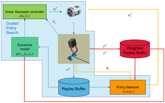
Figure 1.
Schematic diagram of weighted near-optimal experiences policy optimization (WNEPO). Blocks in the blue background are about guided policy search (GPS). WNEPO replaces the replay buffer in GPS with the weighted replay buffer to select the experiences with high quality. When the performance of the policy network is close to that of the linear Gaussian controller, the policy network directly interacts with the environment. In WNEPO, the blue dotted line in the above figure is not executed.
The learning process of the policy network in GPS is essentially supervised learning. The purpose of supervised learning is to train a model to fit the labeled training data so as to achieve a specific task. The degree to which a model performs a task is directly determined by the data fed to it. Consequently, the main drawback of GPS is that the performance of the policy network cannot surpass that of the linear Gaussian controller. Although the near-optimal trajectory samples generated by the linear Gaussian controller will make the policy network explore the high-reward area more fully, which can be very beneficial to improve the sample efficiency, the policy network may never explore the optimal space. Beyond that, the policy network will not be updated online after being deployed to the robot because the performance of the neural network will deteriorate rapidly if low-reward samples are used for fine-tuning. In addition, the policy network will not be updated after it is deployed to the robot because the distribution of the low-reward trajectory samples generated by online interaction is not balanced with the original high-reward near-optimal ones, which will lead to instability of the policy network training.
To solve the problems that GPS encounters, weighted near-optimal experiences policy optimization (WNEPO) is proposed in this paper. The algorithm framework of WNEPO is shown in Figure 1. In WNEPO, the update of the policy network can be divided into two stages. In the first stage, the optimization objective adopted by GPS is used to update the policy network, and the near-optimal experiences generated by the linear Gaussian controller are used as the training samples; in the second stage, the policy network interacts with the environment directly and is trained by the policy gradient method. The first stage of learning is a supervised learning manner—more accurately speaking, imitation learning [20]—and the second stage is a model-free RL manner. Compared with GPS, WNEPO has two improvements: (1) it replaces the traditional replay buffer with a weighted replay buffer; (2) the policy network not only learns from the near-optimal experiences but also uses the data directly interacting with the environment to improve the performance after approaching the performance of the linear Gaussian controller. The pros and cons of the RL algorithms mentioned above are summarized in Table 1.

Table 1.
Advantages and disadvantages of different reinforcement learning (RL) methods.
The goal of this paper is to introduce our WNEPO method through training a biped robot to walk, and the whole work is performed under a MATLAB simulation environment. The paper is organized as follows: Section 1 discusses the shortcomings of the existing algorithms in solving the problem of robot skill learning and describes the overall idea; Section 2 provides a brief introduction to the underlying theory; Section 3 introduces the algorithm framework proposed in detail; Section 4 describes the experimental verification and analysis; Section 5 summarizes the whole paper.
2. Preliminary
In this paper, the reason why WNEPO is introduced in the background of a biped robot walking task is that the state and action dimensions of this task are high, and the system dynamics are nonlinear [21], which puts forward higher requirements for the learning algorithm. Scholars have proposed gait planning methods based on different principles, such as methods based on a mathematical model [22], imitating human walking characteristics [23] and a central pattern generator [24]. All the methods above need accurate modeling and have poor generalization. The RL-based method proposed in this paper can provide some ideas for solving these problems.
Our goal is to have the robot learn to walk in a straight line using minimal control effort without any prior information. As a sequential decision-making problem, this walking task can be modeled as a Markov decision process, where at any moment , the agent in state selects action with probability , causing the environment to enter a new state with state transition probability , and then receives an instantaneous reward [25]. In this paper, we use and instead of and as the control variable and system state, respectively, to be consistent with the conventions in optimal control.
A trajectory is a sequence of state–action pairs along the timeline from until the biped robot enters a terminal state. The quality of robot walking can be evaluated by calculating the reward of trajectory . The reward function used in this paper is inspired by reference [25]. The compound probability of a possible trajectory can be expressed as , where is the policy (or probability) of choosing action in state with the parameter . A real trajectory of robot interaction with the environment is an experience or a sampling trajectory which is stored in the replay buffer for policy learning.
The goal of reinforcement learning is to optimize the parameter in policy that maximizes the expectation of the cumulative reward, which is an optimization problem of Equation (1) [26]:
where is the reward at time , and the discount factor is a real value in [0, 1].
The following of this section focuses on the policy gradient approach, which is widely used in model-free RL and is advantageous in solving high-dimensional robotic problems.
The policy gradient method estimates the gradient of and then updates the parameters using the mini-batch gradient descent. Because policy and environment dynamics are independent of each other, the formula for policy gradient is as follows.
Then, we can update iteratively by calculating using tuples, which is called the minimum decision unit (MDU) in this paper. The gradient descent method is used to update :
In practice, small changes in can lead to dramatic changes in . To achieve a stable improvement in the performance of the policy, it is necessary to limit the Kullback-Leibler(KL) divergence before and after the policy update to a certain threshold value. The corresponding optimization goals are:
where is the pre-update policy. Based on this idea, methods such as Natural Policy Gradient(NPG), Trust Region Policy Optimization(TRPO) [27] and Proximal Policy Optimization(PPO) [28] have emerged. Among them, the PPO algorithm simplifies the optimization problem containing the KL divergence constraint, and the learning process of the policy is more stable.
3. Methods
Our goal was to train a policy network and use it to control the robot to realize the walking skill. The WNEPO proposed in this paper can improve the sample efficiency for robot skill learning, as shown in Figure 1. In this section, we will introduce WNEPO in detail.
To achieve end-to-end control of the robot, the policy is expressed as:
We use a neural network to model . and are the outputs of the neural network, and the two respectively represent the mean and variance used to determine a normal distribution. That is, when the robot is in the state xt, the action ut output by the policy network obeys the normal distribution. The state of the robot can be measured directly by sensors, and this paper considers the sensor observation = and the action to be the torque applied to the joints.
Since the policy is modeled with a neural network, it is usually necessary to construct a large-scale training set first to update the parameters θ. However, in the case of unknown environment dynamics, the sample size obtained from the collection is small and insufficient to train a good performance neural network. To address this issue, we divided the optimization of the policy network into two stages: the imitation phase and the practice phase. In the imitation phase, the policy network learns in a supervised learning manner from the near-optimal trajectories generated by optimizing the linear Gaussian controller. In this way, a policy network with good performance can be trained in the case of small sample size. When the performance of the policy network is close to the linear Gaussian controller, the training process will switch to the next phase. In the practice phase, the network interacts with the environment in a self-exploratory manner. With the help of the weighted replay buffer, the update of the policy network will be more stable.
In the two phases above, a mini-batch of MDUs is sampled randomly from the weighted replay buffer to train the network. Weighted replay buffer plays a key role in the fast and stable learning of a policy network. The following will first discuss the idea of the weighted replay buffer. Then, the details of policy network learning in the imitation phase and the practice phase are analyzed respectively.
3.1. Experience Scoring Algorithm
The original GPS and PPO use random experiences in the replay buffer and discard the old memory according to the first-in-first-out order. This strategy of storing and updating historical data has two major disadvantages: (1) it does not distinguish the quality of the memory experience and uses it indiscriminately, which results in the low efficiency of the replay buffer; (2) discarding memory experiences according to the time sequence and losing the early high-value memory experiences may cause instability of the policy network learning process.
In order to resolve these problems, the experience scoring algorithm is proposed. The experience scoring algorithm evaluates the quality of the experience so as to make more effective use of the trajectories in the replay buffer. For a trajectory , we evaluate its quality from the following three aspects:
- Cumulative discounted reward . The ultimate goal of reinforcement learning is to obtain the maximum cumulative expected reward. It is intuitive to use as an indicator to measure the quality of experience data. For one trajectory, the greater the final cumulative expected reward, the better the overall performance of this episode, and the more valuable it is to learn from.
- The variance of all single step rewards. If the single step reward value is much larger than the average value, it will guide the network update direction from the positive direction more effectively. If the single step reward value is much smaller than the average value, it can guide the network update from the opposite direction more effectively. The reward information close to the average value is less efficient for network updates. The analogy is that people can accumulate more life experience in great success or frustration. However, experiences with too large may lead to more radical network updates and increase the instability of network updating.
- Episode length . There is a correlation between and , but not a positive one. For example, an episode in which the single step reward is always low but lasts for a long time has a larger and a smaller . In this way, even if there is a large , it will not be considered as a valuable trajectory.
The quality of a trajectory can be calculated by the weighted sum of the three evaluation indicators above:
, and are parameters that need to be tuned according to the task.
Figure 2 shows how the weighted replay buffer works based on the experience scoring algorithm. The left side of Figure 2 shows the update process of the traditional experience replay buffer, which stores and discards data similarly to the data structure of a queue, meeting the principle of first-in-first-out. The right side of Figure 2 describes the updating process of the weighted replay buffer. In the weighted replay buffer, the trajectory is the smallest unit to be discarded rather than the MDUs in the traditional replay buffer. More importantly, the data with the highest score are discarded in the weighted replay buffer rather than the data stored first. Besides, the length of the traditional replay buffer is fixed, while the length of the weighted replay buffer is variable. When a new experience with length l is stored in a full traditional replay buffer, the first MDUs will be discarded. However, if this new trajectory is put into the full weighted replay buffer, a complete trajectory with the lowest score will be discarded.
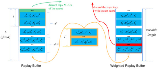
Figure 2.
Comparison of updating processes between traditional replay buffer (left) and weighted replay buffer (right). The yellow line represents the new experiences that will be stored. The green line and the red line represent the experiences that need to be discarded in the traditional replay buffer and the weighted replay buffer, respectively.
3.2. Weighted Near-Optimal Experiences Policy Optimization
After initialization, the policy network learns from the linear Gaussian controller in a supervised learning manner. The linear Gaussian controller is constantly updated in the interaction with the environment, and the near-optimal experiences are stored in the weighted replay buffer. The goal of policy network learning in this phase is to achieve the performance of the linear Gaussian controller. We transformed the original optimization problem as follows.
where . The optimization problem is decomposed into two sub-optimization problems using the Bergman Alternate Direction Multiplier Method (BADMM) [29]:
To facilitate the updating of the Lagrange multiplier , the equation constraint in Equation (8) can be relaxed to the point where the first-order moments of both are equal. Thus, the final optimization problem is:
Before policy network optimization, two sections must be achieved iteratively: dynamics model fitting and linear Gaussian controller optimization.
3.2.1. Dynamics Model Fitting
When the robot interacts with the environment, the stochastic, uncertain nature of the environment itself makes the environment dynamics non-stationary. How the environment dynamics are modeled determines the quality of the trajectory. The universal approximation theorem [30] of neural networks makes it possible to fit any environment dynamics, but training a neural network requires a large number of training samples, which somewhat defeats the purpose of this paper to solve the sample inefficiency problem of robotic skill learning. Considering that linear models can adapt to the environment better than neural networks, but are less generalizable, a Gaussian distribution can be used to represent the uncertainty of the dynamic model. Therefore, this paper uses a linear time-varying system to model the environment.
Assuming that the observed state is Markovian, then the environment dynamics model satisfies:
To estimate parameters of the environment dynamics model, a linear Gaussian controller is used to interact with the environment to obtain trajectories , which, in turn, can construct the input sets and output sets and . Where , , . D is the dimension of the system state space and E is the dimension of the system action space. Based on the linear mean square estimation theory [31], it is known that:
In the above equation, the covariance . The other parameters are calculated as follows:
3.2.2. Linear Gaussian Controller Optimization
If the linear Gaussian controller parameters change too much after the update, it will not be conducive to the convergence of the controller parameters and may also cause unpredictable damage to the robot. Therefore, the KL divergence of the controller before and after the update should be less than a certain threshold value :
where is the controller before the parameter update. Then, we convert the above equation to the Lagrangian dual form [29]:
where is the Lagrange multiplier. Set the cost function equal to:
Therefore, Equation (14) can be abbreviated as:
Since we have fitted the system dynamics model , the parameters of the linear Gaussian controller can be calculated using differential dynamic planning. Define the state value function for any moment t as [32]:
In the equation above, . To find the local minimum of , the action value function is expanded by second-order Taylor at , with:
where is the partial derivative of over and sequentially, and is the Hessian matrix.
To obtain a minimum value for the state value function , the partial derivative of Equation (19) with respect to is:
The parameters of the linear Gaussian controller at moment t are:
Then, substitute Equation (20) for Equation (17):
All parameters of a linear Gaussian controller can be calculated iteratively.
3.2.3. Policy Network Optimization
For the imitation phase, since the policy obeys a Gaussian distribution and the linear Gaussian controller also obeys the distribution , the optimization problem in Equation (9) can be further written as follows.
where , and is the number of trajectories sampled by the system. To simplify the solution of the objective function, the variance of the policy is assumed to be independent of the state . A partial derivative of the above equation yields:
Simplifying the optimization issue to:
It can be seen that when the output of the policy is consistent with the output of the controller, the corresponding policy parameters are the optimal solution to this optimization problem.
For the practice phase, we adopt the PPO-clip algorithm [28]. The whole idea of this approach is to find a functional relationship between policy change and value, take the new policy that can improve the old policy the most and prevent the policy from being updated too much by truncating the policy. In the training process of this phase, the experiences in the weighted replay buffer contains the near-optimal trajectories output by the linear Gaussian controller, as well as the data generated when the policy network interacts with the environment.
We describe the implementation steps of WNEPO as follows:
- (1)
- Initialize the linear Gaussian controller and policy network;
- (2)
- Control the robot to walk with the linear Gaussian controller and record the experiences in the weighted replay buffer;
- (3)
- Use experiences stored in the weighted replay buffer to update the linear Gaussian controller and policy network in a supervised learning manner;
- (4)
- Check whether the cumulative reward obtained by the linear Gaussian controller converges; if it converges, skip to step (5), otherwise return to step (2);
- (5)
- Control the robot to walk with the policy network and record the experiences in the weighted replay buffer;
- (6)
- Use the PPO algorithm to update the policy network until the cumulative reward converges.
The output of the WNEPO algorithm is a policy network, which can directly control the robot to complete the desired task. The implementation steps described above are an experience-based circular process. The pseudo code of the WNEPO algorithm is shown in Algorithm 1.
| Algorithm 1. WNEPO: A two-phase framework for efficient robotic skills learning |
| 1: Initialize , , , weighted replay buffer D |
| 2: Initialize , K, J, |
| 3: For : |
| 4: Initialize |
| 5: Interacting with the environment M times with |
| 6: collect , update |
| 7: fit dynamics to D |
| 8: For : |
| 9: Update the linear Gaussian controller with Equation (16) |
| 10: If : |
| 11: Optimize with Adam according to Equation (25) |
| 12: Else: |
| 13: Interacting with the environment N times with |
| 14: collect , update |
| 15: Randomly pick minibatch sequences from D |
| 16: Update based on PPO |
| 17: Update |
| 18: End For |
| 19: End For |
4. Experiments
In this section, we will answer the following three questions by carrying out simulation experiments on a MATLAB platform: (1) Can a biped robot learn walking skills only from the imitation phase without any prior knowledge? (2) Can the WNEPO algorithm make the robot learn better walking skills in a shorter time? From the perspective of RL, are asymptotic performance and sample efficiency better? (3) How do weighted near-optimal experiences affect the performance of different algorithms?
4.1. Experiment Setup
4.1.1. Description of the Environment
The WNEPO proposed in this paper will be validated with a simulation experiment of a biped robot, which was built using MATLAB’s Simscape toolbox. The biped robot is shown in Figure 3. The robot was required to stay upright during walking and walk as far as possible in a straight line within a limited time, during which the motors of each joint execute the torque output by the policy network.
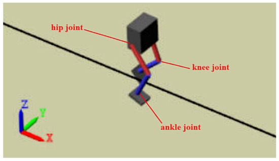
Figure 3.
Simulation environment. The robot’s body and ground can be regarded as the environment. The motor at the three joints (ankle, knee and hip) of each leg can be regarded as the agent. Our task is to make the motor output an appropriate torque to control the robot to walk along a straight line.
The robot had two legs and a torso, and each leg contained three joints (ankle, knee and hip). Torque (Nm) was applied to each joint of the leg, i = 1, 2, …, n. The key physical property parameters of the robot are shown in Table 2.
Table 2.
Physical property parameters of the biped robot.
The environment provided 29 observations for action decision, including: (1) Y (lateral) and Z (vertical) translations of the torso center of mass; (2) X (forward), Y (lateral) and Z (vertical) translation velocities; (3) Yaw, pitch and roll angles of the torso; (4) Yaw, pitch and roll angular velocities of the torso; (5) Angular positions and velocities of the three joints (ankle, knee and hip) on both legs; (6) Action values from the previous time step.
The contact between the robot feet and the ground adopted a point-to-surface contact mode, and the contact stiffness and damping were 500 (N/m) and 50 (Ns/m), respectively. In order to make the walking task closer to a real situation, Gaussian white noise was added to the contact stiffness and damping.
4.1.2. Parameter Specification
PPO has strong robustness, so the neural network structure and other hyperparameters had little influence on the training process. Various network structures, including a three-layer network and a four-layer network, were tested, and there was no significant difference in the training effect, so the default network structure commonly used by PPO, i.e., the policy network and the critic network, both use two hidden layers, with 300 and 400 nodes, respectively. The output layer of the network is six nodes, representing the moments applied to a total of six joints in both legs; the output layer of the evaluation network has only one node and is a score of the current state.
Set the capacity of weighted replay buffer D to 600 and mini-batch size to 500. The maximum episode is 5000. The values of , and are 0.4, 0.5 and 0.1, respectively.
The reward function with the following expression:
where is the displacement in the x-direction, y is the distance of the trajectory from the preset line, is the normalized vertical translation displacement of the robot center of mass, is the sample time of the environment and is the final simulation time of the environment. was set to 10 s in this simulation.
Both the policy and value networks were trained using Adam, with a learning rate of 0.0001 for the policy network and 0.002 for the value network. The order of the trajectory data in the experience pool was not scrambled in order to ensure that the complete sequence fragments could be taken for the estimation of the generalized advantage function.
4.1.3. Comparison Methods
WNEPO can be regarded as the combination of model-free and model-based RL, which can give full play to the advantages of sample efficiency of model-based RL and the asymptotic performance of model-free RL. In order to evaluate the performance of WNEPO, we compared it with the following algorithms:
- iLQG [19]. iLQG is a typical model-based RL algorithm. When the environment dynamics are known, the optimal analytical solution can be obtained.
- GPS [6]. GPS is a state-of-the-art algorithm combining model-based RL with model-free RL.
- WE-GPS. Replaces the experience pool in GPS with a weighted replay buffer.
- PPO [28]. State-of-the-art model-free on-policy RL algorithm. This paper does not consider off-policy RL methods because off-policy RL usually encounters higher risks, which is not suitable for robot skills learning [33].
- In practice, the last point can make a big difference if mistakes are costly—e.g., you are training a robot not in simulation, but in the real world. You may prefer a more conservative learning algorithm that avoids high risk if there is real time and money at stake if the robot were to be damaged.
- WE-PPO. Replaces the replay buffer in PPO with a weighted replay buffer.
- GPS-PPO. GPS is used to update the policy network offline, and then, the PPO algorithm is used to train the policy network online. The only difference between GPS-PPO and WNEPO is that GPS-PPO directly uses the online interactive data between the policy network and the environment instead of the experiences in the weighted replay buffer to update the policy.
4.2. Result
4.2.1. Evaluation of Walking Skills Learned from the Imitation Phase
The optimization process of the linear Gaussian controller is shown in the following Figure 4.
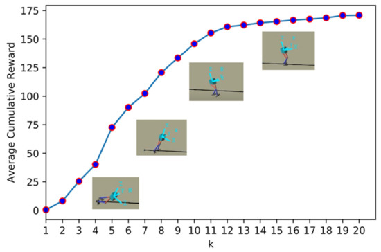
Figure 4.
The optimization process of the iterative linear Gaussian controller (iLQG). With the increase in interaction data between the iLQG controller and the environment, more experiences are used to fit the dynamics, and the average cumulative reward of the iLQG agent is multiplying. When the interaction experiences accumulated to a certain amount, the performance improvement of iLQG is unobvious.
At the beginning of the iteration, an accurate dynamics model was unavailable and the output torque was small. The agent only explored near the initial configuration to avoid possible damage to the robotic system. After a period of interaction, the controller tried to control the robot to walk, but it was unable to complete the walking task because the dynamics model was inaccurate. Therefore, the trajectories generated by the controller were far from optimal. With the increase in samples in the weighted experience replay buffer, the dynamics model was fitted more and more accurately. After eight iterations (k ≥ 8), the robot could walk a distance, although the behavior seemed unnatural. After 12 iterations (k ≥ 12), the average cumulative reward of the linear Gaussian controller had nearly converged.
In the process of the iLQG interacting with the environment, the policy network is simultaneously trained using samples obtained from the iLQG’s experiences. Since the average cumulative reward of the iLQG controller almost converges when k = 12, we evaluated the walking skills learned by the policy network at this time. The training process of the policy network can be regarded as a typical regression problem. We used root-mean-square error(RMSE) loss function to evaluate how well the policy network imitates the iLQG controller. The RMSE curve of policy network training is shown in Figure 5 for when k = 12. It can be seen that the policy network converges when epoch = 9, which means that the performance of the policy network is close to the iLQG controller. Next, we used the policy network to control the robot directly, and we take a trajectory as an example to analyze the movement of the biped robot.
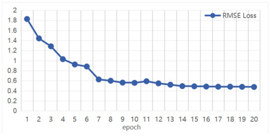
Figure 5.
RMSE loss curve in policy network training. In this paper, we set epoch = 20.
Walking gait refers to the posture and behavior characteristics of walking, including the continuous activities of hip, knee and ankle. Figure 6 shows the joint forces exerted on the six joints of the biped robot during walking. It can be seen from the figure that the torque exerted on the ankle joint is periodic, because the two feet alternately support the robot to move forward during the movement. The torque applied to the knee joint does not change periodically because the robot needs to adjust the torque of the knee joint in real time to ensure body balance. The torque exerted on the hip joint is the smallest, and the direction of the torque applied to the left hip joint and the right hip joint is always opposite, which is consistent with the characteristics of human walking.
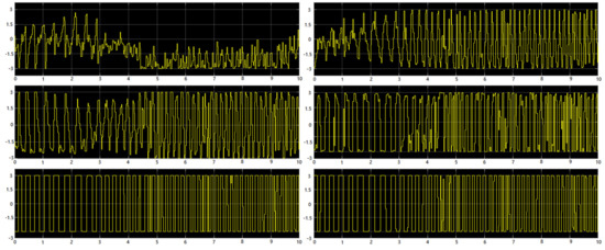
Figure 6.
The torque applied to the leg joints during a walk. The three pictures on the left show the torque applied to the left hip joint, left knee joint and left ankle joint from top to bottom. The three pictures on the right show the torque applied to the right hip joint, right knee joint and right ankle joint from top to bottom. The abscissa represents the movement time in seconds.
Figure 7 shows the motion of the robot. Figure 7a shows the lateral offset. It can be found that the robot moves in the positive direction of the y-axis in the process of moving forward. The maximum offset is 0.36 m, which can be ignored compared with the total distance. Figure 7b shows how the center of gravity changes over time. At the beginning of the movement, the center of gravity changes greatly because the robot needs to adapt to the state change from the initial standing state to the walking state. However, after 5 s, the change in gravity center is controlled in the range of 0.005 m, which indicates that the robot can deal with the uncertainty of the environment and effectively adjust its own posture to complete the walking task. Figure 7c shows that the robot’s speed is uneven during the forward process, which may be caused by the lateral offset of the robot. The robot needs to make a trade-off between moving forward and maintaining body balance.
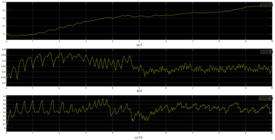
Figure 7.
The state of the robot during one trajectory. The three figures from top to bottom are the lateral deviation, the change in gravity center and the forward speed of the robot.
Even so, the robot can walk a longer distance and move more smoothly at this time. It can be considered that the trajectories generated by the linear Gaussian controller at this moment are near-optimal. In the next subsection, we will use more indicators to evaluate whether the robot walking skills can be further improved in practice phase.
4.2.2. Asymptotic Performance and Sample Efficiency
When the performance of the linear Gaussian controller tends to converge, we enter the practice phase from the imitation phase. The role of the iLQG controller now is to expand the weighted replay buffer D to provide high-value trajectories for policy network training. Different from the traditional PPO, the experiences used for policy network optimization are not only from the interaction between the robot itself and the environment but also from the near-optimal trajectories generated by the iLQG controller.
Figure 8 demonstrates the training process of different algorithms. It shows that the iLQG controller has the fastest convergence rate and can achieve a reward expectation of close to 170 using fewer training samples and less computational power. The method proposed in this paper can hardly surpass the performance of the linear Gaussian controller during the imitation phase. This result is intuitive because the learning samples determine the upper limit of the model performance. GPS and WE-GPS encounter the same situation in the training process.
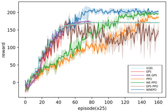
Figure 8.
Comparison of our method and prior methods on bipedal robot walking task.
The policy network can achieve higher reward than iLQG after switching to the practice phase. In the practice phase, the performance of GPS and WE-GPS is limited by the performance of the linear Gaussian controller. WNEPO can use the exploration mechanism of model-free RL to let the robot experience more situations that have not been seen before. This will help the neural network to search the global optimal policy better, which makes it more robust than the linear Gaussian controller when facing unseen situations. WNEPO obtains higher reward than the current best-performing on-policy model-free RL method, PPO. The reason is that the parameter update process of the policy network uses both near-optimal experiences and online interactive experiences.
The comparison of these algorithms in learning walking skills is shown in Table 3. In this experiment, we required the robot to keep upright and walk as far as possible in 10 s. When all the policies converged, 30 trials were run under different environment parameters (contact stiffness and damping), and the average value was calculated. WNEPO achieved the best asymptotic performance and achieved the longest walking distance with the least control output.
Table 3.
Comparison of asymptotic performance and sample efficiency.
At the same time, we know from Table 2 that the sample efficiency of WNEPO is significantly improved compared to PPO. Although the sample efficiency of WNEPO is worse than that of GPS, our biggest concern is to better learn motor skills, so more online interaction is obviously desirable.
Finally, we will discuss the role of the weighted replay buffer in WNEPO. The role of the weighted replay buffer in the imitation phase can be reflected by comparing the performances of WNEPO and GPS. It can be seen that the weighted replay buffer helps to make the performance of the policy network closer to the iLQG controller. This phenomenon can be explained as the experience of a high score helping the policy network not to be trapped in low-reward states. The role of the weighted replay buffer in the practice phase can be illustrated by the performance of GPS-PPO in Figure 8. The online interaction of GPS-PPO makes the training process fluctuate greatly, and there is still no convergence until the maximum number of episodes is reached. It can be inferred that the use of a weighted replay buffer can improve training stability in the practice phase. The results in Figure 8 also show that the weighted replay buffer can improve the performances of GPS and PPO. The weighted replay buffer is a plug-and-play module which can be widely used for other RL algorithms.
5. Conclusions
In this paper, a two-phase framework for efficient learning of robot skills is proposed based on reinforcement learning, which we call WNEPO. WNEPO can be regarded as the combination of model-free RL and model-based RL. In the imitation phase, the policy network uses the near-optimal experiences of the linear Gaussian controller to update the parameters, which is more efficient than PPO. By continuing to train the policy network with the model-free RL algorithm in the practice phase, the robot can better learn walking skills than with other algorithms. The weighted replay buffer proposed in this paper plays a key role in the policy network training process. The weighted replay buffer is used to store the historical experience data with high scores so as to improve the training stability and strengthen the exploration of high-reward areas.
The advantage of our method is that the environment dynamics do not need to be known in advance and highly robust skills can be learned through fewer interactions with the environment. The weighted replay buffer proposed has been proved to be a plug-and-play module that can be used in other RL algorithms.
In order to further tap into the potential of the weighted replay buffer, in future work, we will conduct a theoretical analysis on the tuning method of the three parameters in the experience-scoring algorithm. In addition, we will also test the effect of the WNEPO algorithm in other robot skill-learning situations, such as high-dimensional manipulation tasks.
Author Contributions
Conceptualization, L.H.; methodology, L.H.; software, L.H. and H.Z.; validation, L.H. and H.Z.; formal analysis, L.H. and H.W.; investigation, L.H.; resources, L.H. and H.W.; data curation, L.H. and H.Z.; writing—original draft preparation, L.H.; writing—review and editing, H.W. and Q.W.; visualization, L.H.; supervision, H.W.; project administration, H.W.; funding acquisition, L.H. and H.W. All authors have read and agreed to the published version of the manuscript.
Funding
This research was funded by the Industrial Commissioner Program of Changsha Science and Technology Bureau of Hunan Province (grant No. CSKJ2017-42), the National Basic Research Program of China (grant No. 2013CB035504), the Fundamental Research Funds for the Central Universities of Central South University (grant No. 2019zzts252) and Shenzhen Jiade Equipment Technology Co., Ltd.
Institutional Review Board Statement
Not applicable.
Informed Consent Statement
Not applicable.
Data Availability Statement
Not applicable.
Conflicts of Interest
The authors declare no conflict of interest.
References
- Kuindersma, S.; Deits, R.; Fallon, M.; Valenzuela, A.; Dai, H.; Permenter, F.; Koolen, T.; Marion, P.; Tedrake, R. Optimization-based locomotion planning, estimation, and control design for the atlas humanoid robot. Auton. Robot. 2016, 40, 429–455. [Google Scholar] [CrossRef]
- Raibert, M.; Blankespoor, K.; Nelson, G.; Playter, R. Bigdog, the rough-terrain quadruped robot. IFAC Proc. Vol. 2008, 41, 10822–10825. [Google Scholar] [CrossRef]
- Miller, A.T.; Knoop, S.; Christensen, H.I.; Allen, P.K. Automatic grasp planning using shape primitives. In Proceedings of the 2003 IEEE International Conference on Robotics and Automation, Taipei, Taiwan, 14–19 September 2003; pp. 1824–1829. [Google Scholar]
- Saxena, A.; Driemeyer, J.; Ng, A.Y. Robotic grasping of novel objects using vision. Int. J. Robot. Res. 2008, 27, 157–173. [Google Scholar] [CrossRef]
- Kober, J.; Bagnell, J.A.; Peters, J. Reinforcement learning in robotics: A survey. Int. J. Robot. Res. 2013, 32, 1238–1274. [Google Scholar] [CrossRef]
- Levine, S.; Finn, C.; Darrell, T.; Abbeel, P. End-to-end training of deep visuomotor policies. J. Mach. Learn. Res. 2016, 17, 1334–1373. [Google Scholar]
- Kalashnikov, D.; Irpan, A.; Pastor, P.; Ibarz, J.; Herzog, A.; Jang, E.; Quillen, D.; Holly, E.; Kalakrishnan, M.; Vanhoucke, V.; et al. Scalable deep reinforcement learning for vision-based robotic manipulation. In Proceedings of the 2018 Conference on Robot Learning, Zürich, Switzerland, 29–31 October 2018; pp. 651–673. [Google Scholar]
- Schoettler, G.; Nair, A.; Ojea, J.A.; Levine, S. Meta-Reinforcement Learning for Robotic Industrial Insertion Tasks. arXiv 2020, arXiv:2004.14404. [Google Scholar]
- Cho, N.; Lee, S.H.; Kim, J.B.; Suh, I.H. Learning, Improving, and Generalizing Motor Skills for the Peg-in-Hole Tasks Based on Imitation Learning and Self-Learning. Appl. Sci. 2020, 10, 2719. [Google Scholar] [CrossRef]
- Peng, X.B.; Berseth, G.; Yin, K.; Panne, M.V.D. Deeploco: Dynamic locomotion skills using hierarchical deep reinforcement learning. ACM Trans. Graph. 2017, 36, 1–13. [Google Scholar] [CrossRef]
- Zhang, M.; Geng, X.; Bruce, J.; Caluwaerts, K.; Vespignani, M.; SunSpiral, V.; Abbeel, P.; Levine, S. Deep reinforcement learning for tensegrity robot locomotion. In Proceedings of the 2017 IEEE International Conference on Robotics and Automation, Singapore, 29 May–3 June 2017; pp. 634–641. [Google Scholar]
- Liu, N.; Cai, Y.; Lu, T.; Wang, R.; Wang, S. Real–Sim–Real Transfer for Real-World Robot Control Policy Learning with Deep Reinforcement Learning. Appl. Sci. 2020, 10, 1555. [Google Scholar] [CrossRef]
- Abbeel, P.; Coates, A.; Quigley, M.; Ng, A.Y. An application of reinforcement learning to aerobatic helicopter flight. In Proceedings of the 2006 International Conference on Neural Information Processing, Vancouver, BC, Canada, 4–7 December 2006; pp. 1–8. [Google Scholar]
- Zhang, M.; Vikram, S.; Smith, L.; Abbeel, P.; Johnson, M.; Levine, S. SOLAR: Deep structured representations for model-based reinforcement learning. In Proceedings of the 2019 International Conference on Machine Learning, Long Beach, CA, USA, 9–15 June 2019; pp. 7444–7453. [Google Scholar]
- Thuruthel, T.G.; Falotico, E.; Renda, F.; Laschi, C. Model-based reinforcement learning for closed-loop dynamic control of soft robotic manipulators. IEEE Trans. Robot. 2018, 35, 124–134. [Google Scholar] [CrossRef]
- Clavera, I.; Rothfuss, J.; Schulman, J.; Fujita, Y.; Asfour, T.; Abbeel, P. Model-Based Reinforcement Learning via Meta-Policy Optimization. In Proceedings of the 2018 Conference on Robot Learning, Zürich, Switzerland, 29–31 October 2018; pp. 617–629. [Google Scholar]
- Asadi, K.; Misra, D.; Kim, S.; Littman, M.L. Combating the compounding-error problem with a multi-step model. arXiv 2019, arXiv:1905.13320. [Google Scholar]
- Levine, S.; Vladlen, K. Learning complex neural network policies with trajectory optimization. In Proceedings of the 2014 International Conference on Machine Learning, Beijing, China, 21–24 June 2014; pp. 829–837. [Google Scholar]
- Todorov, E.; Li, W. A generalized iterative LQG method for locally-optimal feedback control of constrained nonlinear stochastic systems. In Proceedings of the 2005 American Control Conference, Portland, OR, USA, 8–10 June 2005; pp. 300–306. [Google Scholar]
- Kajita, S.; Hirukawa, H.; Harada, K. Introduction to Humanoid Robotics; Springer Press: Berlin/Heidelberg, Germany, 2014. [Google Scholar]
- Heess, N.; Dhruva, T.B.; Srinivasan, S.; Jay, L.; Josh, M.; Greg, W.; Yuval, T. Emergence of Locomotion Behaviours in Rich Environments. arXiv 2017, arXiv:1707.02286. [Google Scholar]
- Kaneko, K.; Kanehiro, F.; Kajita, S.; Yokoyama, K.; Akachi, K.; Kawasaki, T.; Ota, S. Design of prototype humanoid robotics platform for HRP. In Proceedings of the 2002 International Conference on Intelligent Robots and Systems, Lausanne, Switzerland, 30 September–4 October 2002; pp. 2431–2436. [Google Scholar]
- Choi, M.; Lee, J.; Shin, S. Planning biped locomotion using motion capture data and probabilistic roadmaps. ACM Trans. Graph. 2003, 22, 182–203. [Google Scholar] [CrossRef]
- Taga, G. A model of the neuro-musculo-skeletal system for anticipatory adjustment of human locomotion during obstacle avoidance. Biol. Cybern. 1998, 78, 9–17. [Google Scholar] [CrossRef] [PubMed]
- Sutton, R.S.; Barto, A.G. Reinforcement Learning: An Introduction; MIT Press: Cambridge, MA, USA, 2018. [Google Scholar]
- Schaal, S. Is imitation learning the route to humanoid robots? Trends Cogn. Sci. 1999, 3, 233–242. [Google Scholar] [CrossRef]
- Schulman, J.; Levine, S.; Abbeel, P.; Jordan, M.; Moritz, P. Trust region policy optimization. In Proceedings of the 2015 International Conference on Machine Learning, Lille, France, 6–11 July 2015; pp. 1889–1897. [Google Scholar]
- Schulman, J.; Wolski, F.; Dhariwal, P.; Radford, A.; Klimov, O. Proximal policy optimization algorithms. arXiv 2017, arXiv:1707.06347. [Google Scholar]
- Wang, H.; Banerjee, A. Bregman Alternating Direction Method of Multipliers. In Proceedings of the 2014 International Conference on Neural Information Processing, Montreal, QC, Canada, 8–13 December 2014; pp. 2816–2824. [Google Scholar]
- Zainuddin, Z.; Ong, P. Function approximation using artificial neural networks. WSEAS Trans. Math. 2008, 7, 333–338. [Google Scholar]
- Stamatis, C. A general approach to linear mean-square estimation problems. IEEE Trans. Inform. Theory 1973, 19, 110–114. [Google Scholar]
- Balogun, O.S.; Hubbard, M.; DeVries, J.J. Automatic control of canal flow using linear quadratic regulator theory. J. Hydraul Eng. 1988, 114, 75–102. [Google Scholar] [CrossRef]
- Wang, Y.; Li, T.S.; Lin, C. Backward Q-learning: The combination of Sarsa algorithm and Q-learning. Eng. Appl. Artif. Intell. 2013, 26, 2184–2193. [Google Scholar] [CrossRef]


Publisher’s Note: MDPI stays neutral with regard to jurisdictional claims in published maps and institutional affiliations. |
© 2021 by the authors. Licensee MDPI, Basel, Switzerland. This article is an open access article distributed under the terms and conditions of the Creative Commons Attribution (CC BY) license (http://creativecommons.org/licenses/by/4.0/).