Abstract
A CFD model to simulate the cooling technique trough slot jet impingement has been developed. Such a technique has been tested on an existing vertical galvanizing industrial line, which initially envisaged a round jet configuration, the subject of a previous work. Two different slot jet configurations have been simulated and compared to the pre-existing one, in order to provide design information for a possible new jet cooler after exploring different solutions. The numerical model has been appropriately calibrated and validated by comparing it with experimental measurements from a literature case. At first, a single slot jet configuration was simulated through a 2D model, then multi slot configurations were calculated using 3D models. Different turbulence models were compared to select the best candidate for the CFD approach. Finally, several configurations with different slots numbers and jet-wall distances were considered. It was possible to understand the physical mechanisms underlying this cooling technique and to be able to select the most promising configuration for the reference industrial cooling process.
1. Introduction
The jet impingement heat exchange mechanism consists of the impact of a liquid or gas flow against a certain surface, in order to ensure a significant thermal or mass energy transfer between the fluid and the surface. At a given fluid velocity, the jet impingement produces a higher heat exchange coefficient than a similar convective flow parallel to the surface. For this reason, it is widely used in industrial applications, such as raw material cooling during the formation process or cooling of electronic components, heat treatments, heating of optical surfaces for defrosting, cooling of gas turbine components and many others. The jet impingement is very effective in the region where the flow impacts the thinnest boundary layer; moreover, in the surrounding area a higher turbulence zone is created, and consequently higher energy exchanges are generated.
The flow structure out of a nozzle or opening impacts on the target surface by passing through distinct regions, as schematized in Figure 1. Inside the jet there is a region not affected by the momentum transfer, called the core region [1]. The jet zone that includes the shear layer and the core region is called the initial free jet; it is followed by a decaying jet phase, present from a variable distance between 4 and 8 diameters from the nozzle outlet, where the axial velocity decreases in the central part and the profile tends to a Gaussian curve. In this region the axial velocity and the jet width vary linearly with the axial position. Martin [2] provided an equation to predict the velocity value in the free and decaying jet regions, for low Reynolds flows. Viskanta [3] has subdivided this region into two zones, called the initial developing zone and fully developed zone, where the decaying free jet reaches a velocity profile similar to a Gaussian curve. Subsequently, when the flow reaches the wall, it loses axial velocity and it curves in the so-called stagnation region. The static pressure increases near the wall; these proximity effects are transmitted upstream. According to Martin [2], the stagnation zone extends laterally 1.2 times the nozzle diameter. From the stagnation zone, laterally to the wall, the flow curves and enters the wall jet region. The minimum thickness of the wall jet is located between 0.75 and 3 diameters away from the jet axis, then it tends to thicken moving away from the nozzle. The wall jet boundary layer is influenced outwards by the velocity gradients with respect to the fluid outside the wall jet and by the velocity gradients near the wall.
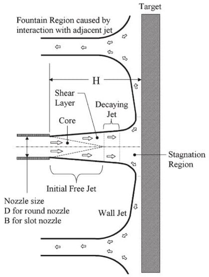
Figure 1.
Flow regions of a jet impingement [1].
Experimental surveys obtained by Katti and Prabhu [4] investigated the radial Nusselt distribution within the jet by varying the Reynolds number and the jet distance from the wall. They identified a maximum in correspondence with the stagnation region, because in this area the boundary layer thickness is at minimum. A secondary peak may be present at a certain distance; several numerical and experimental studies have focused on this phenomenon [5,6,7,8,9]. The laminar boundary layer (in the stagnation point) becomes turbulent after a transition region, which leads to an improvement in the mass transfer in the normal direction to the wall. Furthermore, in the wall jet region, the flow bend accelerates the stream causing a heat exchange increase. Heat exchange intensity decreases because the cross-sectional flow area in the jet region increases. Experiments performed by Hoogendorn [10] found that the turbulence development in the free jet influences the local trend of heat exchange and the Nusselt number in the stagnation region. For shaped nozzles at a high distance from the wall (H/D > 5) or for jets from a long pipe, the Nusselt trend has a peak just on the jet axis. For shaped nozzles placed close to the wall, with low inlet turbulence (Tu ~ 1%), the maximum Nusselt value is reached in the range 0.4 < r/D < 0.6, while a local minimum (95% of the peak value) is located at r = 0. Numerical simulations performed by Abe and Suga [11] show that mass and heat transfer in the deceleration zone is dominated by large-scale eddies, in contrast to the wall jet phenomena, where the shear stresses are dominant.
Most of the literature studies conducted on the jet impingement phenomenon concern single circular jets, while less effort of research is devoted to the slot jet configuration, as in Figure 2. Slot jet configuration consists of a long slot having a width B, which creates a long and thin jet, with a two-dimensional velocity profile. From a theoretical point of view, a single round jet concentrates the heat exchange in the impingement area, while a slot jet configuration guarantees a more uniform exchange. Theoretical and experimental researches on such an impingement configuration have been found and can be mentioned following a time evolution. Gardon et al. [12] and Sparrow et al. [13] measured the Nusselt distribution by varying the main influence parameters. Quinn [14] studied the aspect ratio influence on outflow problems from rectangular flared outflow jets. Liakos et al. [15,16,17] developed a mathematical model for calculating the heat release in turbulent impinging premixed flames by comparing different eddy viscosity turbulence models and including the thermal radiation. Zhou and Lee [18] carried out experiments on rectangular jets, flared by 45° at the outlet, in order to investigate the flow structure and the heat exchange, by varying the nozzle-wall distance and the Reynolds number. Senter and Solliec [19] experimentally investigated the flow field of a confined turbulent slot air jet impinging normally on a moving flat surface. Experiments were conducted for a nozzle-to-plate spacing of eight slot nozzle widths, at three jet Reynolds numbers (Re = 5300, 8000, and 1.06 × 10⁴) and four surface-to-jet velocity ratios of 0, 0.25, 0.5, and 1. It appeared that the flow field patterns at a given surface-to-jet velocity ratio are independent of the jet Reynolds number in the range of 5300–1.06 × 10⁴. A slight modification of the flow field was observed for a surface-to-jet velocity ratio of 0.25 whereas at higher ratios of 0.5 and 1, the flow field was significantly affected. Sharif and Banerjee [20] investigated numerically the heat transfer due to a confined turbulent slot-jet impinging on a hot moving plate for a range of the jet exit Reynolds number, plate velocity, and jet to plate distance, using the standard k-ε turbulence model with enhanced wall treatment to calculate the eddy viscosity. Dutta et al. assessed various RANS based turbulence models for a slot jet impinging flow at the two values of nozzle to plate spacing [21]. Gorman et al. [22] focused on jet-axis switching, for which a non-circular free jet is faced with a major change of shape as the downstream distance from the plane of jet origination increases. A comparative study of different Reynolds averaged Navier-Stokes (RANS) based turbulence models has been carried out by Achari and Das [23] by numerically simulating a two-dimensional turbulent slot jet impinging air normally on a flat plate, to obtain information about the performance which can be obtained with such an approach. Slot impingement heat transfer has been investigated numerically in the cases of moving plate or moving nozzle separately by Rahimi and Soran [24]. Pachpute and Premanchadran [25] present experimental and numerical investigations of slot air jet impingement cooling of a circular heated cylinder, taking into account a semi-circular confinement to improve the heat transfer rate behind the cylinder. The confined jet impingement heat transfer with different nozzle-plate spacing is also considered by Huang et al. [26] focusing on the intermittency transition model and crossflow transition model in applying a RANS method.
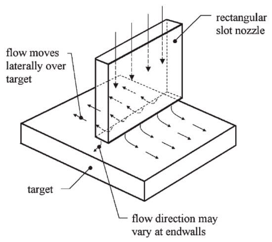
Figure 2.
Slot jet configuration.
Therefore, there is a relative abundance of numerical analyses on slot jet configurations, mainly focused on reference geometries and turbulence investigations. The application of slot jets to industrial processes is still under development. Indeed, the extensive use of CFD can provide significant support in the development of industrial components, based on fluid dynamics and heat transfer phenomena, as its support to glass production and galvanizing of metal bands testifies [27,28,29,30]. A CFD model, able to simulate the slot jet in different configurations, has been developed. Initially, a single slot has been considered with a 2D model, then a multi-slot jet with two or three slots has been simulated with 3D models. Several distances of the jet from the target surface have been investigated. Moreover, different turbulence models have been considered and discussed, in order to identify the most appropriate model. The numerical results have been compared with the measurements from Gardon and Akfirat [12]. In addition, the slot jet configuration has also been compared with the round jet configuration, developed in a previous work [30] which describes the advantages and merits of one or the other geometry. The CFD model developed for the slot jet impingement technique has been applied on an existing vertical galvanizing industrial line designed with round jets clusters [30] in order to test the present technique on a practical configuration.
2. Governing Equations
The Reynolds-averaged equation for conservation of mass and momentum form the dynamic flow problem. The energy equation must be considered to take into account the heat exchange mechanisms. The main parameter used to evaluate the convective heat exchange is the Nusselt number, defined as:
where B is the characteristic dimension of the jet (the diameter for a round jet impingement or the width for a slot jet), λ the thermal conductivity of the fluid, while h is the local or average coefficient of convective heat exchange, calculated as follows:
The previous dimensionless parameter (Nu) usually depends on the Reynolds number (3) and Prandtl number (4):
where Uj is the average velocity of the outgoing jet. The reference properties of the fluid are taken at the jet outlet. Three turbulence models have been compared: realizable k-ε, k-ω SST and v2f. The first and the second are based on the Boussinesq’s hypothesis to model the Reynolds stress tensor and are also called “linear eddy viscosity models”. The v2f model is a “non-linear eddy viscosity model”.
2.1. Realizable k-Epsilon Turbulence Model
The realizable k-ε model differs from the standard k-ε model for two reasons: the formulation of the turbulent viscosity and the transport equation of ε are modified, because it is derived from an exact equation for the vorticity fluctuations computation [31,32]. The term “realizable” is because the model satisfies certain mathematical constraints on viscous stresses, in accordance with the turbulent flow physics. The transport equations for the turbulent kinetic energy (k) and its dissipation rate (ε) are:
where:
The eddy viscosity is defined as in the other k-ε turbulent models, as:
However, the main difference is in the definition of Cµ, that is calculated with the following formulas:
where A0 and As are constant. The other model constants are: C1ε = 1.44, C2 = 1.9, σk = 1.0 and σε = 1.2.
2.2. k-Omega SST Turbulence Model
This model was developed to combine the accuracy of the k-ω model near the wall and the robustness of the k-ε in the free-stream. It contains some different terms with respect to the standard k-ω formulation. A blending function activates the transformed models k-ω and k-ε depending on the local value of y+, i.e., near or far from the wall [33]. A different formulation for the eddy viscosity and modified constants are introduced. The transport equations are:
The diffusivity is obtained by the following equations:
The eddy viscosity is determined with:
The model constants are: σk,1 = 1.176, σω,1 = 2.0, σk,2 = 1.0, σω,2 = 1.168, α1 = 0.31, βi,1 = 0.075 and βi,2 = 0.0828.
2.3. v2f Turbulence Model
This turbulence model was developed in more recent times and it is particularly used for jet impingement problems. Behnia [34] has performed numerous researches on jet impingement, showing the excellent results from this turbulence model in 2D axisymmetric cases. The peculiarity of this model is the use of the term v2, which replaces the turbulence kinetic energy k for the eddy viscosity calculation. The quantity v2 can be interpreted as the fluctuation of velocity perpendicular to the current lines. This term allows the right magnitude to be kept regarding the damping of turbulence transport near the wall. The transport equations for k, ε, v2 and f (elliptic relaxation function) are reported:
where:
The turbulent length and time scales are defined as follows:
The values of the constants and turbulent Prandtl numbers are: α = 0.6, C1 = 1.5, C2 = 0.3, Cε1 = 1.5, Cε2 = 1.9, Cη = 70, Cµ = 0.22, CL = 0.23, σk = 1 and σε = 1.3. Finally, the eddy viscosity and the term C’ε1 are defined as:
3. Experimental Setup and Numerical Models
3.1. Experimental Apparatus: Test Case
The test case used to validate the CFD model is from [12] and is briefly presented. Figure 3 shows the measurement apparatus used to obtain the experimental data, consisting of a plenum designed to dampen pressure oscillations, followed by a duct, which shrinks up to the slot width B.
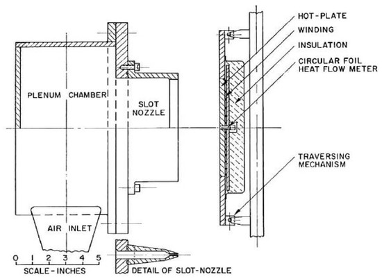
Figure 3.
Experimental test apparatus [12].
The jet from the slot impacts an aluminum plate, an excellent conductor, so as to suppress the temperature differences on its sides; this plate is heated electrically, while the back and sides are thermally insulated. Its temperature is controlled at 36 [°F] higher than the outlet nozzle temperature, low enough to be able to neglect the radiation heat losses. The convective heat exchange is therefore obtained from the interaction between a cooling air flow and an isothermal hot surface. A transducer mounted on the plate, sliding on the latter, allows the local heat exchange coefficient calculation. The measurements were made for different slot openings, equal to 1/4, 1/8 and 1/16 inch, with a slot length fixed to 6 inches. In addition to the single slot, tests were conducted on rows of slots, arranged in different ways: two slots (placed at a distance of 4 inches) or three slots (separated by 2 inches).
3.2. CFD Models
A crucial aspect is the ability to correctly replicate the slot outlet conditions (velocity profile). For this reason, an upstream extension of the computational domain has been adopted (Figure 4); it essentially consists of a plenum. Downstream of it there is a duct, at the top of which a restricted section is mounted to accelerate the flow and to assume the geometry configuration of the slot.
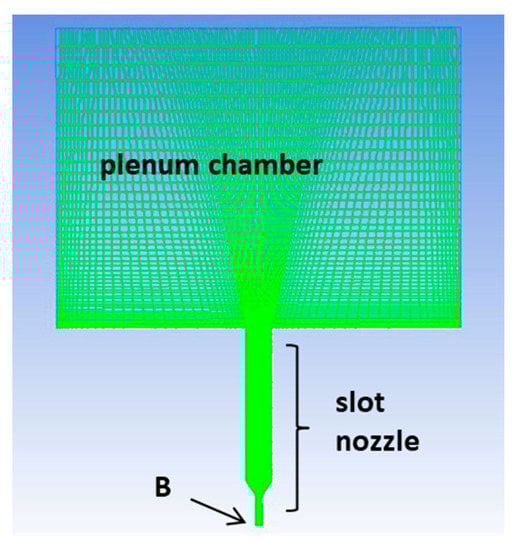
Figure 4.
Calculation domain for the velocity profile slot jet generation.
A 2D plane grid equivalent to the real 3D case was adopted for the single slot configuration. The velocity profile is developed only in the vertical direction, while the orthogonal variation is entirely negligible. Steady simulations with the following boundary conditions were set. Inlet mass flow rate condition ṁ = 0.197 [kg/s] (calculated from the Reynolds number at the outlet jet Re = 1.1 × 10⁴, at temperature 30 [°C] with B = 3.175 [mm]) on the three plenum rectangular sides (excluding the lower side) with turbulence intensity equal to 1%. On the side opening B a pressure ambient outlet condition was fixed with temperature of 30 [°C]. All the remaining walls were set as adiabatic no-slip boundaries. This simulation provides the velocity profile to fix as boundary condition in the simulations of the slot jet impingement problem.
In Figure 5 the computational domain with the relative grid for the jet impingement study is shown. A multi-block structured mesh was generated using Ansys v. 17 platform. A further thickening in the jet area and near the target surface (where the jet impacts) was introduced. The proper wall treatment is guaranteed by y+ values close to one. The total mesh size amounts to about 900 kCells.
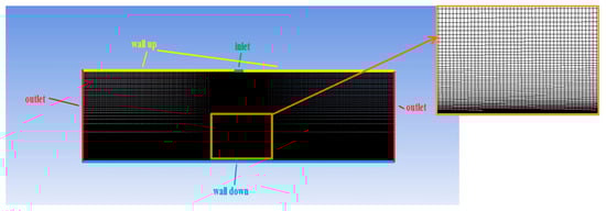
Figure 5.
Computational grid of a single slot configuration.
In Figure 5 the patches of the following boundary conditions were also highlighted. In the outlet jet (green) the velocity and turbulence profile (k and ε) generated by the previous upstream model with the plenum was set. On the lateral surfaces, placed sufficiently far from the jet axis (20 times), the outlet ambient pressure was imposed. The upper surface was set as adiabatic wall free slip, while on the target surface (to be cooled) a wall no-slip condition with constant temperature of 50 [°C] was imposed, to match with the test case [12]. All the governing and transport equations were solved with SIMPLE second order pressure based computational schemes using Ansys Fluent v 17 code. The modeled fluid is air treated as an ideal gas, the viscosity is computed with Sutherland’s law and the specific heat with a polynomial law to consider temperature variations.
4. Single Slot Analysis
The numerical simulations were performed initially on a single slot configuration in order to calibrate the turbulence model by comparing the numerical data to the experimental measurements [12]. This analysis supports the understanding of the main flow dynamic phenomena that occurs in a slot impingement. Only H/B = 8 was considered for this scope, while different jet-walls distances will be analyzed for the multi-slot jet case.
In Figure 6 the convective heat transfer coefficient distributions obtained by the different turbulent models were compared to the experimental values.
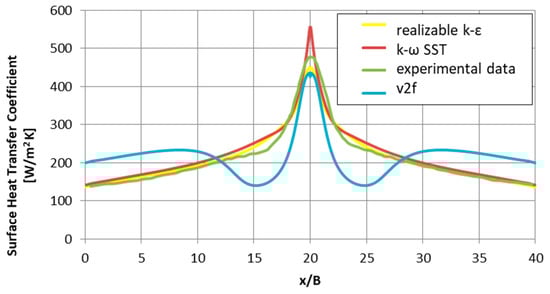
Figure 6.
Comparison between the numerical results and the experimental values [12] on the convective heat transfer coefficient, for H/B = 8, Re = 1100.
The realizable k-ε and the SST turbulent models can predict the trend of the convective heat transfer coefficient with good accuracy with respect to the experimental measurements, while a notable discrepancy has been found with the v2f model. In the latter case, the largest difference occurs close to the area where streamlines have the highest curvature. For this reason, this model appears less suitable for the slot impingement application; unlike the other two RANS models; the percentage errors with respect to the experiments are reported in Table 1.

Table 1.
Percentage errors with respect the experimental measurements for the single slot case with H/B = 8, Re = 1.1 × 10⁴.
The most accurate model with reference to the experimental data is the k-ε (error below 1% on the average value of the heat exchange coefficient). The maximum peak (concerning the jet axis) is slightly underestimated by this model. However the SST model also offers a good match in the average value, but it lacks accuracy in the prediction of the maximum value (overestimated by 16.43%). In Figure 7 the velocity contours of the slot jet are reported for H/B = 8 with the k-ε model.
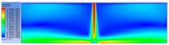
Figure 7.
Velocity contours of the single slot jet at H/B = 8, Re = 1.1 × 10⁴, with k-ε model.
For this jet-wall distance the flow can interact with the surrounding stagnant fluid, which is transported by viscous effects on the edge of the jet. Near the impact to the surface, due to the higher static pressure gradient in the stagnation region, the flow bends and forms the wall jet region; here the boundary layer develops along the jet-axis distance. Moreover, within this zone there is an acceleration of the flow (orange colors), that starts with a velocity peak near the wall (when the boundary layer is not developed) and then gradually lowers, due to the boundary layer thickening. In Figure 8 the corresponding turbulent kinetic energy contour is shown to discuss the heat transfer.
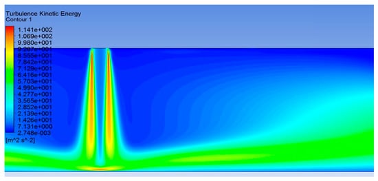
Figure 8.
Turbulence kinetic energy contours of the single slot jet at H/B = 8, Re = 1.1 × 10⁴, with k-ε model.
It can be noted that the maximum generation of turbulence kinetic energy is located where the flow from the opening is mixed with the surrounding stagnant fluid and forms a shear layer. In the stagnation zone there is the maximum heat exchange coefficient; here the boundary layer is not yet developed and does not interact with to the flow close to the surface. Near the wall jet there is a flow acceleration and a stronger interaction with the surrounding stagnant gas that supports more significant turbulent kinetic energy production.
Comparison of a Single Slot Jet and a Single Round Jet Configuration
The flow physics of the jet impingement is strongly affected by the nozzle geometry. In this paragraph the numerical results obtained by a slot jet and by a round jet are compared. The same jet-wall distance, Reynolds number and outlet conditions have been considered in order to evaluate the performance of each case, as reported in Table 2.
Table 2.
Summarizing of the main parameters for the comparison of a slot jet and a round jet.
The same settings were used both for the grid and for the numerical models. In the round jet configuration, a circular duct long enough to develop the flow was used to obtain the velocity and turbulence profiles. More details on the circular nozzle were reported in a previous paper [34], which also highlighted the best accuracy of the v2f model for those cases. In Figure 9 the Nusselt number distributions for the two configurations are compared for the jet–wall distances H/B = H/D = 2 (left) and 6 (right); in Table 3 the average Nusselt values and percentage differences are shown.
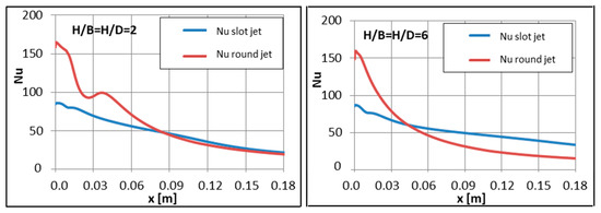
Figure 9.
Nusselt trend comparison between slot and round jet, for H/B = H/D = 2 (left) and 6 (right).
Table 3.
Average Nusselt number comparison between round and slot jet with its percentage difference for different jet-wall distance.
For the configuration with low jet-wall distance (H/D = H/B = 2) the circular nozzle guarantees a higher average Nusselt number than the slot jet, due to the greater heat exchange near the jet axis (higher peak). In fact, there is a higher impact in the area near the jet, which has less chance of mixing with the surrounding stationary environment. The heat transfer distribution is not much lower than that of the slot jet, also at a certain distance from the axis. On the other hand, for a higher jet-wall distance (H/D = H/B = 6) the situation is considerably different. The round jet maintains a considerably higher Nusselt peak; in this case the outgoing flow has more space to mix with the stationary surrounding fluid (this advantage decreases moving away from the jet axis). For this configuration, the slot jet has higher performance and guarantees a uniform distribution with a higher average Nusselt number (16.5%). This better heat transfer uniformity leads to an effective advantage if the distance between the wall and the slot is not excessively low, otherwise the best impact in correspondence to the jet axis, guaranteed by the circular nozzle, also leads to a higher average Nusselt number.
5. Multi Slot Jet Analysis
In this section, multiple slot jet configurations (with two or three jets) are analyzed. To include interaction phenomena between the various jets 3D models are considered. Table 4 shows the fundamental parameters of the multi slot jet configurations.
Table 4.
Fundamental parameters of the multi slot jet configurations.
Figure 10 shows the domain and the mesh used for the multi slot analysis. The grid has the same characteristics as the single slot case, i.e., structured multi-block and a wall treatment with a y+ close to one. The mesh size consists of about 2.5 million cells. The same CFD settings were also imposed. The main difference on boundary conditions concerns the symmetry condition imposed to save computational resources; the slot length in Figure 10 is half of 152.4 [mm] (from Table 4), as well as the central slot width. The velocity and the turbulence profile obtained from a previous 3D plenum simulation were imposed at the inlet.
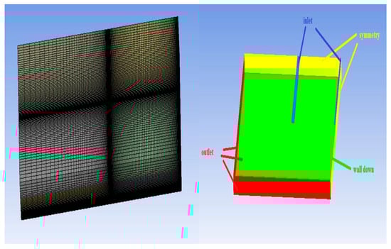
Figure 10.
Calculation domain for the multi slot jet (three jets), H/B = 4.
5.1. H/B = 4
In this section the cases with three and two slot jets H/B = 4, are analyzed and correspond to the slot close to the target wall. In Figure 11 the velocity contours of the three slots (upper) and two slots (down) configurations are shown.
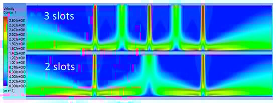
Figure 11.
Velocity contours of multi slot jet configuration with H/B = 4, Re = 5500 and realizable k-ε model: three slots (upper) and two slots (down).
Since the slots are close to the wall, the fluid cannot mix considerably with the surrounding medium, so the jet is well developed in the wall proximity. The single jet physics is therefore kept in this case, but the interaction between the jets is also present and the wall jets meet. Away from the jet axis, the wall velocity decreases inside the wall jet because of the boundary layer development, leading to an unfavorable pressure gradient ∂p/∂x > 0. In the mixing area between the wall jets there is a local pressure increase and the flow tends to curve upwards to leave the upper outlet (where pressure ambient is set).In this regards the pressure contours (with the surface streamlines projected) of the three slots (upper) and two slots (down) configurations are shown in Figure 12, while in Figure 13 the velocity vector in the mixing zone has been reported.
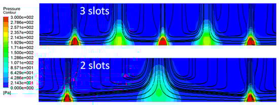
Figure 12.
Pressure contours and surface streamlines of multi slot jet configuration with H/B = 4, Re = 5500 and realizable k-ε model: three slots (upper) and two slots (down).
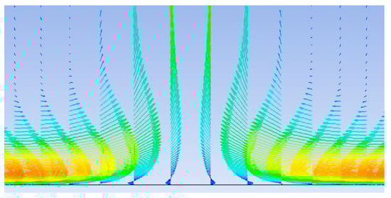
Figure 13.
Velocity vector focus on the meeting zone between two wall jets.
The main differences between the three and two slot configurations concern the distance between the jets; in the two jets it is almost doubled, so the wall jets have more space to reduce their velocity (interacting with the surrounding medium) before their interaction and their mixing. The turbulent kinetic energy contours for the two configurations (Figure 14) highlight these differences for the heat transfer.
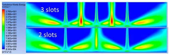
Figure 14.
Turbulent kinetic energy contours of multi slot jet configuration with H/B = 4, Re = 5500 and realizable k-ε model: three slots (upper) and two slots (down).
In the descending path of the jet towards the wall, there is a shear layer that is not too strong (due to the jet proximity to the wall). A turbulent kinetic energy production is evident in the wall jet areas where the flow accelerates and interacts with the surrounding fluid. The zone with the maximum production corresponds to the interfering zones of the wall jets. This maximum is lower in the case of two jets because of the higher jet distance, and the turbulence production is more uniformly distributed.
In Figure 15 the convective heat transfer coefficient distributions from the CFD simulations are compared with the experimental data; in Table 5 the average values are reported together with the corresponding percentage error with respect to the experiments.
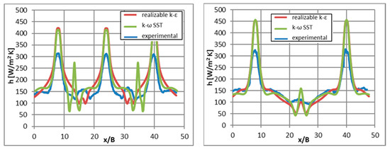
Figure 15.
Comparison between numerical and experimental data of the convective heat transfer coefficients for the multi slot configurations with H/B = 4 and Re = 5500: 3 slots (left) and 2 slots (right).
Table 5.
Average heat transfer coefficient and percentage errors of the CFD models with respect the experiment of the multi slot jet configurations for H/B = 4.
The heat exchange peaks of Figure 15 are striking in correspondence of the jets for all the numerical simulations and the experimental measurements. There are intermediate peaks for both configurations, where the wall jets merge. In the three slots configuration the intermediate peaks of the numerical simulations show the highest deviation with respect to the experimental trend; boundary layer separations develop in those zones and are difficult to be accurately solved by the numerical approach. The SST model overestimates the heat transfer coefficient increase and predicts a maximum closer to the external slot rather than about halfway between the consecutive slots (as with the k-ε and experimental cases). In the two-slot configuration the distributions are more similar to the single slot case, because the interaction between the jets is weaker. The above inaccuracy on the intermediate peaks is therefore lower than in the three slots configuration. An overestimation in the jet peaks for the two slots configuration is obtained from the numerical models. Good accuracy has been obtained in the last configuration for the average values of the convective heat transfer coefficient, (percentage error always below 4%) while a higher error is shown for the three slots configuration due to a worse prediction of the intermediate peaks.
5.2. H/B = 16
The same analysis has been performed for a configuration with the jets with higher distance from the target wall defined by H/B = 16. Three or two jets have been considered. In Figure 16 the velocity contours and streamlines of the three slots configuration have been reported.
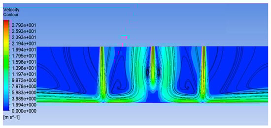
Figure 16.
Velocity contours and streamlines of three slot jets configuration with H/B = 16, Re = 5500 and realizable k-ε model.
The developed flow field in this case is clearly different with respect the closest jet-wall case. The external jets have more space to mix with the surrounding fluid and to lose velocity before their impingement on the target surface. In addition, the central jet is subject to an even stronger mixing; the streamlines of the external wall jets curve upwards, affected by the pressure increase in the stagnation zone of the central jet. The central jet not only interacts with the surrounding fluid, but also with the wall jets that entrain it towards the upper outlet. This last phenomenon increases the turbulent kinetic energy in the upper zones significantly, as shown in Figure 17.
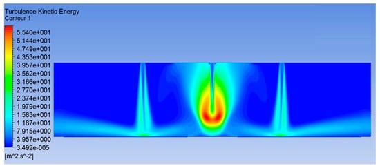
Figure 17.
Turbulent kinetic energy contours of three slot jets configuration with H/B = 16, Re = 5500 and realizable k-ε.
Similar contours for the configuration with two slots are obtained. It is clear that the wall jets have a lower energy at a higher jet-wall distance and their interaction is weaker due to the higher distance between the jets. In Figure 18 the convective heat transfer coefficient distributions are compared with the experimental data; in Table 6 the average values are reported with the corresponding percentage error referred to in experimental values.
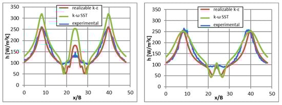
Figure 18.
Comparison between numerical and experimental data of the convective heat transfer coefficients for the multi slot configurations with H/B = 16 and Re = 5500: 3 slots (left) and 2 slots (right).
Table 6.
Average heat transfer coefficient and percentage errors of the CFD models with respect to experimental values of the multi slot jet configurations for H/B = 16.
In the three jets configuration the k-ε turbulent model gives the best prediction of convective heat transfer coefficient, almost coincident with the experimental value for a large area, including the external jets regions. A larger deviation is detected in the central jet with both models (more evident for SST), due to the pressure gradient between the stagnation region and the surrounding fluid. Also, for the two slots configuration the overall match with numerical and experimental data is good except for the region where there is a strong streamlines curvature (caused by the overpressure of the wall jets that interact and merge). In this zone the jet interaction is weaker due to the larger distance from the wall and because of the jets’ mutual distance. In the two slots configurations the percentage errors are quite small for both models, with an underestimation by the k-ε and an overestimation by the SST model.
From the above results and discussion, the k-ε model is selected for the application of the CFD approach to a reference industrial case.
6. Industrial Jet Cooler Module Optimization
The CFD model is applied to an existing vertical galvanizing industrial line to understand the effect of the slot impingement technique. The slot impingement technique has been optimized and compared to the existing round jet cooling solution. In a previous work [30] the same module has been described in detail. The module is responsible for the temperature control of a moving band trough HNX jets (a mixing of 95% nitrogen and 5% hydrogen) to avoid oxidation of the target metal. The existing jet cooler is composed of 16 plenums, with 16 jet round nozzles each (256 in total) and a length of the metal band of 1650 [mm]. In order to save computational resources a quarter sector of 32 jets has been considered. Periodic boundary conditions on side walls are set to focus the analysis on the central area module. The entire jet cooler is modeled along the axial direction of the band. The new jet cooler based on slot impingement is designed taking some geometrical dimensions as constraints from the existing plant, as reported in Table 7.
Table 7.
Main parameters of the industrial model.
From the above data, the slots number for the cooling sector have been optimized. The total mass flow rate of the 256 round jets has been fixed to the slots in order to compare the different configurations. Unlike the round jets model, in the slot model it is not possible to place a single suction mouth for the operating fluid, located in the end of the band. In fact, the slot geometry, characterized by a transversal development equal to the band, forces the outgoing flow to curve in the longitudinal direction. A suction mouth is required between one slot and another, otherwise the jets would be deviated with no impingement on the band. For this reason, the plenum for each single slot must be designed accordingly. In Figure 19 the plenum geometry that feeds the slot is shown.
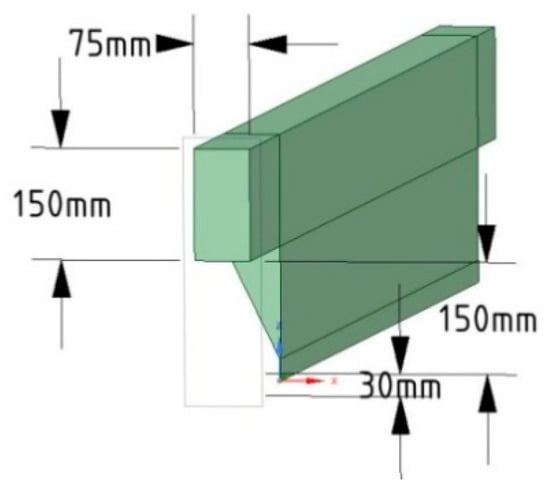
Figure 19.
Plenum configuration upstream of each slot.
The geometry is designed with a constant narrow channel to guarantee a fully developed velocity profile, equal for each slot. Two different multi slot jet configurations (Table 8) have been simulated and compared to the existing configuration with round jets.
Table 8.
Main parameters of the two industrial configurations tested.
The actual jet cooler geometry was simplified and the domain includes only the fluid flow from the outlet nozzles to the band surface, as well as the solid domain of the band (band half thickness). The above main parameters were chosen in order to make the present configurations comparable to the previous one with round jets [30]. The parameters guarantee the same mass flow rate and similar jet velocity values from the plenum. In the second model the H/B ratio was nevertheless strongly reduced with respect to the reference value [30] to enhance the turbulence generation into the flow field. To decrease H/B, the slot width was increased, with same jet height (a constraint design parameter). The Discrete Ordinates radiation model was activated in the CFD model due to the high band temperature. A mesh of two million elements complies with wall refinement constraints to get a y+ value close to one. The following boundary conditions were set: at the inlet the velocity and turbulence profile obtained in the preliminary simulation on the plenum model (Figure 19) have been set. Due to the band movement, the transverse input surface was modeled by activating the Frame Motion option with a velocity of 180 [m/min] in the appropriate direction. The temperature of 660 [°C] was fixed on this transverse input surface of the band. The band solid domain (with half thickness) is equipped with meshes and the conjugate heat transfer option is considered. The moving wall option with a speed equal to that of the band has been activated for the band upper surface. On the lower band surface a symmetry condition was used to correctly simulate the cooling on both band sides. An outlet relative pressure condition of 150 [Pa] (pressure value controlled in the cooling chamber) was set on the boundaries of flow domain between one slot and the other. The periodicity condition on the lateral surfaces of the band and on the transversal surfaces of the flow is imposed (the model represents only a sector of the complete jet cooler in the middle of the line).
The fluid is a nitrogen-hydrogen mixture, therefore the transport equations for each species were introduced. An ideal gas mixture with thermo-physical properties varying with the temperature according to the ideal gas mixing law is considered. Figure 20 and Figure 21 show the development of the streamlines in the flow domain for both configurations. The flow structure, already described in the previous paragraphs, is evident with the wall jets at the target surface; they interact and deviate towards the upper outlet, due to the induced pressure. Figure 22 shows the temperature patterns along the band, for the slot jet configurations compared to the existing one with round jets.
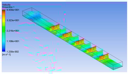
Figure 20.
Streamlines in the configuration #1 with 5 slots.
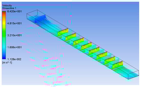
Figure 21.
Streamlines in the configuration #2 with 8 slots.
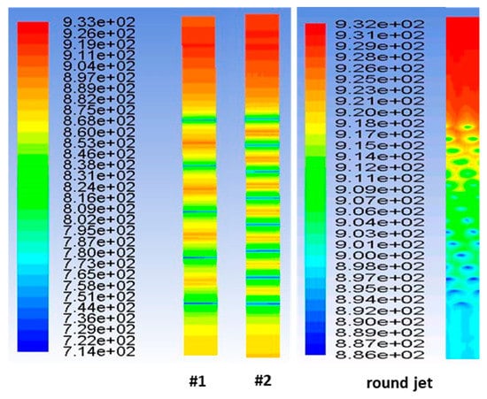
Figure 22.
Temperature contours on the tape for the different cooling configurations.
The temperature gradients along the sliding direction are stronger in the slot jet configurations, with peak values close to 700 [K] in the jet area. In fact, with the same global cooling mass flow rate, in the round jets model the impinging jet is distributed over 32 nozzles, a much higher number than in the configurations with slot jets. In the two slot jet configurations, it should be noted that for eight slots a lower minimum temperature value is reached than that for five slots, due to a local speed difference of 20 [m/s]. As for the transverse temperature distribution, the slot configuration has a more uniform trend than the round jet nozzles. This feature offers a mechanical advantage by limiting transverse deformations, which could jeopardize the product quality. Figure 23 shows the surface temperature distributions along the flow direction and Table 9 reports the main quantities needed to evaluate the heat exchange of the different configurations.
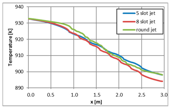
Figure 23.
Temperature contours on the tape surface along its movement direction.
Table 9.
Main thermal parameters obtained in the different configurations.
The results obtained from the simulations show that the lowest temperature at the tape outlet is found with eight slot jets. In fact, in this case a higher average convective heat transfer coefficient is obtained over the entire band surface with respect to the other configurations. The heat transfer coefficient has been evaluated according to Equation (2), with the radiant heat flux subtracted from the overall. On the other hand, the round jets configuration gives the maximum value of the heat transfer coefficient on the target surface only. As previously discussed, slot jets offer better results for higher jet-wall distances. A larger temperature gradient is found in the external parts of the impingement plane, while the differences between the distributions of Figure 23 are negligible.
7. Conclusions
The flow mechanism of the heat transfer associated to the slot jet impingement on a target surface has been discussed in some detail and a reference CFD model, validated against experimental data, has been setup. The CFD model has been used to simulate the cooling of an existing vertical galvanizing industrial line through the slot jet impingement technique. Two different configurations with several slot jets have been simulated and compared to the existing system. The validated CFD model can be used to develop correlations for the slot jet impingement that are rarely available in open literature. The simulation approach has been used to understand benefits and flaws of different configurations to demonstrate its interest in the design of industrial cooling system based on this technology. The slot jet impingement is made more effective and advantageous by increasing the jet-wall distance which leads to more uniform transversal temperature distributions, ensuring less mechanical deformations and a higher product quality.
Author Contributions
The authors have equally contributed to the concept of the research activity, the setup of the model, the discussion of the results and the writing of the paper. All authors have read and agreed to the published version of the manuscript.
Funding
This research was funded by University of Sassari by “2019 Una Tantum extraordinary funding for Research”.
Institutional Review Board Statement
Not applicable.
Informed Consent Statement
Not applicable.
Acknowledgments
Danieli Centro Combustion Spa–Genova–has provided the reference geometry and data for the industrial configuration. Only a limited set of results has been published due to confidentiality reasons. The technical support from Danieli and the useful discussions during the research activity are warmly acknowledged.
Conflicts of Interest
The authors declare no conflict of interest.
Nomenclature
| B | Slot width |
| D | Diameter |
| h | Convective heat transfer coefficient |
| H | Height |
| k | Turbulent kinetic energy |
| ṁ | Mass flow rate |
| Nu | Nusselt number |
| p | Pressure |
| Pr | Prandtl number |
| q | Heat flux |
| r | Radius |
| Re | Reynolds Number |
| T | Temperature |
| Tu | Turbulence intensity |
| u | Velocity |
| x | Coordinate |
| y+ | Wall non dimensional distance |
| α | Thermal diffusivity |
| ε | Rate of dissipation of turbulent kinetic energy |
| λ | Thermal conductivity |
| ν | Kinematic viscosity |
| ρ | Density |
| ω | Specific rate of dissipation |
References
- Zuckerman, N.; Lior, N. Jet impingement heat transfer: Physics, correlations and numerical modeling. Adv. Heat Transf. 2006, 39, 566–630. [Google Scholar]
- Martin, H. Heat and mass transfer between impinging gas jets and solid surfaces. Adv. Heat Transf. 1977, 13, 1–60. [Google Scholar]
- Viskanta, R. Heat transfer to impinging isothermal gas and flame jets. Exp. Therm. Fluid Sci. 1993, 6, 111–113. [Google Scholar] [CrossRef]
- Katti, V.; Prabhu, S.V. Experimental study and theoretical analysis of local heat transfer distribution between smooth flat surface and impinging air jet from a circular straight pipe nozzle. J. Heat Mass Transf. 2008, 51, 4480–4495. [Google Scholar] [CrossRef]
- Gao, N.; Sun, H.; Ewing, D. Heat transfer to impinging round jets with triangular tabs. Int. J. Heat Mass Transf. 2003, 46, 2557–2569. [Google Scholar] [CrossRef]
- O’Donovan, T.S.; Murray, D.B. Jet impingement heat transfer—Part I: Mean and root-mean-square heat transfer and velocity distributions. Int. J. Heat Mass Transf. 2007, 50, 3291–3301. [Google Scholar] [CrossRef]
- O’Donovan, T.S.; Murray, D.B. Jet impingement heat transfer—Part II: A temporal investigation of heat transfer and local fluid velocities. Int. J. Heat Mass Transf. 2007, 50, 3302–3314. [Google Scholar] [CrossRef]
- Gao, N.; Ewing, D. Investigation of the effect of confinement on the heat transfer to round impinging jets exiting a long pipe. Int. J. Heat Fluid Flow 2006, 27, 33–41. [Google Scholar] [CrossRef]
- Bovo, M.; Etemad, S.; Davidson, L. On the numerical modeling of impinging jet heat transfer. In Proceedings of the International Symposium on Convective Heat and Mass Transfer in Sustainable Energy, Yasmine Hammamet, Tunisia, 26 April–1 May 2009. [Google Scholar]
- Hoogendorn, C.J. The effect of turbulence on heat transfer at a stagnation point. Int. J. Heat Mass Transf. 1977, 20, 1333–1338. [Google Scholar] [CrossRef]
- Abe, K.; Suga, K. Large eddy simulation of passive scalar in complex turbulence with flow impingement and flow separation. Heat Transf. Asian Res. 2001, 30, 402–418. [Google Scholar] [CrossRef]
- Gardon, R.; Akfirat, J.C. Heat transfer characteristics of impinging two dimensional air jets. J. Heat Transf. 1966, 88, 101–108. [Google Scholar] [CrossRef]
- Sparrow, E.M.; Wong, T.C. Impingement transfer coefficients due to initially laminar slot jets. Int. J. Heat Mass Transf. 1975, 18, 597–605. [Google Scholar] [CrossRef]
- Quinn, W.R. Turbulent free jet flows issuing from sharp-edged rectangular slots: The influence of slot aspect ratio. Exp. Therm. Fluid Sci. 1992, 5, 203–215. [Google Scholar] [CrossRef]
- Liakos, H.H.; Founti, M.A.; Markatos, N.C. Modeling the characteristic types and heat release of stretched premixed impinging flames. Comput. Mech. 2001, 27, 88–96. [Google Scholar] [CrossRef]
- Souris, N.; Liakos, H.; Founti, M.; Palyvos, J.; Markatos, N.C. Study of impinging turbulent jet flows using the isotropic low-Reynolds number and the algebraic stress methods. Comput. Mech. 2002, 28, 381–389. [Google Scholar] [CrossRef]
- Liakos, H.H.; Keramida, E.P.; Founti, M.A.; Markatos, N.C. Heat and mass transfer study of impinging turbulent premixes flames. Heat Mass Transf. 2002, 38, 425–432. [Google Scholar] [CrossRef]
- Zhou, D.W.; Lee, S.J. Forced convective heat transfer with impinging rectangular jets. Int. J. Heat Mass Transf. 2006, 50, 1916–1926. [Google Scholar] [CrossRef]
- Senter, J.; Solliec, C. Flow field analysis of a turbulent slot air jet impinging on a moving flat surface. Int. J. Heat Fluid Flow 2007, 28, 708–719. [Google Scholar] [CrossRef]
- Sharif, M.A.R.; Banerjee, A. Numerical analysis of heat transfer due to confined slot-jet impingement on a moving plate. Appl. Therm. Eng. 2009, 29, 532–540. [Google Scholar] [CrossRef]
- Dutta, R.; Dewan, A.; Srinivasan, B. Comparison of various integration to wall (ITW) RANS models for predicting turbulent slot jet impingement heat transfer. Int. J. Heat Mass Transf. 2013, 65, 750–764. [Google Scholar] [CrossRef]
- Gorman, J.M.; Sparrow, E.M.; Abraham, J.P. Slot jet impingement heat transfer in the presence of jet-axis switching. Int. J. Heat Mass Transf. 2014, 78, 50–57. [Google Scholar] [CrossRef]
- Achari, A.M.; Das, M.K. Application of various RANS based models towards predicting turbulent slot jet impingement. Int. J. Therm. Sci. 2015, 98, 332–351. [Google Scholar] [CrossRef]
- Rahimi, M.; Soran, R.A. Slot jet impingement heat transfer for the cases of moving plate and moving nozzle. J. Braz. Soc. Mech. Sci. Eng. 2016, 38, 2651–2659. [Google Scholar] [CrossRef]
- Pachpute, S.; Premachandran, B. Experimental and numerical investigations of slot jet impingement with and without a semi-circular bottom confinement. Appl. Therm. Eng. 2018, 132, 352–367. [Google Scholar] [CrossRef]
- Huang, H.K.; Sun, T.Z.; Zhang, G.Y.; Sun, L.; Zong, Z. Modeling and computation of turbulent slot jet impingement heat transfer using RANS method with special emphasis on the developed SST turbulence model. Int. J. Heat Mass Transf. 2018, 126, 589–602. [Google Scholar] [CrossRef]
- Basso, D.; Cravero, C.; Reverberi, A.P.; Fabiano, B. CFD analysis of regenerative chambers for energy efficiency improvement in glass production plants. Energies 2015, 8, 88945–88961. [Google Scholar] [CrossRef]
- Cravero, C.; De Domenico, D.; Leutcha, P.J.; Marsano, D. Strategies for the numerical modelling of regenerative pre-heating systems for recycled glass raw material. Math. Model. Eng. Probl. 2019, 6, 324–332. [Google Scholar] [CrossRef][Green Version]
- Cogliandro, S.; Cravero, C.; Marini, M.; Spoladore, A. Simulation strategies for regenerative chambers in glass production plants with strategic exhaust gas recirculation system. Int. J. Heat Technol. 2017, 35, S449–S455. [Google Scholar] [CrossRef]
- Carozzo, G.; Cravero, C.; Marini, M.; Mazza, M. CFD Simulation of a Temperature Control System for Galvanizing Line of Metal Band Based on Jet Cooling Heat Transfer. Appl. Sci. 2020, 10, 5248. [Google Scholar] [CrossRef]
- Launder, B.E.; Spalding, D.B. Mathematical Models of Turbulence; Academic Press: London, UK, 1972. [Google Scholar]
- Rodi, W. Turbulence models and their application in hydraulics. A state-of-the-art review. In IAHR Monograph Series, 3rd ed.; Taylor & Francis: Rotterdam, The Netherlands, 2000. [Google Scholar]
- Ansys Fluent Theory Guide v.17; ANSYS Inc.: Canonsburg, PA, USA, 2013.
- Behnia, M.; Parneix, S.; Durbin, P.A. Simulation of Jet Impingement Heat Transfer with the k-ε-ν2f Model. In Center for Turbulence Research Annual Research Briefs; Stanford University: Stanford, CA, USA, 1996. [Google Scholar]


Publisher’s Note: MDPI stays neutral with regard to jurisdictional claims in published maps and institutional affiliations. |
© 2021 by the authors. Licensee MDPI, Basel, Switzerland. This article is an open access article distributed under the terms and conditions of the Creative Commons Attribution (CC BY) license (http://creativecommons.org/licenses/by/4.0/).