Local Sensitivity Analysis of Steady-State Response of Rotors with Rub-Impact to Parameters of Rubbing Interfaces

Abstract

Local sensitivity analysis, which describes the relative importance of specific design parameters to the response of systems, is crucial for investigating dominant factors in optimal design. In this paper, local sensitivity analysis of the response of rotors with rub-impact to parameters of rubbing interfaces is carried out. The steady-state motion of the rotor is evaluated by a harmonic balance method and the sensitivity coefficients for every rotation speed over the speed range are derived analytically. Two classical models, including the Duffing oscillator and the gap model, are utilized to validate the accuracy and capability of the adopted methods and high accuracy is shown. Numerical investigations of sensitivities of steady-state response of rotors to parameters of rubbing interfaces are then carried out, based on a lumped Jeffcott rotor and a finite element model respectively. Conclusions are drawn that the response of rotors subjected to rubbing problems is more sensitive to initial clearance than other parameters of the applied friction model. With increase of initial gap, the response of rotors becomes more sensitive and the range of region subjected to rub-impact forces shrinks until the separation of rotor and stator.

1. Introduction

For the purpose of searching for optimal design parameters for rotating machinery, investigations of the dynamic characteristics of the system, such as stability analysis [1,2], reliability analysis [3] and optimal design analysis [4] based on specific criteria, have been performed by many scholars. Typically, a sensitivity analysis is also suggested when researching the dynamic characteristics of a system. Sensitivity analysis can provide quantitative information about to what extent does the responses of rotating system change when the design parameters varies from a base case, thus dominant impact factors can be found based on a restricted number of cases rather than enormous amount of data. In general, there are two different kinds of methods measuring sensitivities of the investigated system, i.e., local and global sensitivity analysis [5,6]. Local sensitivity analysis, which is in the topic of this paper, is performed by investigating the influence of slight deviation from nominal values of different design parameters on the output parameters, i.e., the maximum amplitudes of certain degrees of freedom.

Many scholars have contributed to the applications of sensitivity analysis to specific domains. Su [7] et al. proposed a method to assess the extent of rotor failure and investigated the frequency reliability sensitivity with respect to several stochastic parameters. Melchers and Ahammed [8] presented a structural sensitivity analysis approach based on moment and compared the results with those computed by a conventional Monte Carlo method. Lataillade [9] et al. combined sensitivity analysis with Monte Carlo methods by introducing a supplementary procedure. Petrov [10,11] et al. investigated the sensitivity of the steady response of bladed disk assemblies with respect to parameters of nonlinear friction contact interfaces. Leister [12] et al. proposed a new sensitivity analysis method for a rotor supported by two bearings. Yang and Sievert [13] studied the sensitivity of large turbine shaft system with respect to shaft unbalance. Pan [14] et al. applied sensitivity analysis to investigate the influence of the mass and the offset of disk on rotors. And results have revealed that the offset of disk influence the critical speed in a significant way. Papini [15] et al. carried out a sensitivity analysis on solid rotor induction machines. Ying [16] et al. investigated the load change sensitivities of a multi-support system utilizing virtual displacement principle. Based on the model they proposed, the influence of load variation on dynamic characteristics and sensitivities of a multi-support structure is researched. Anusonti-Inthra [17] et al. carried out sensitivity analysis and uncertainty qualification for a coaxial rotor system, where the sensitivities of hub loads with respect to ambient drift speed, rotor angular speed and center of gravity location on the blade are investigated.

Furthermore, rubbing phenomenon is expected when the clearance between rotor and stator becomes so small that friction and collision happens at interfaces. It makes the response of rotor strongly nonlinear and is sensitive to parameters of friction interfaces. Investigations of dynamic analysis for rotors with rub-impact have been performed by many researchers. Choy and Padovan [18] found that the rub-impact becomes more severe with increase of imbalance of rotor. Dai [19] et al. presented that the increase of excitation force would result in the transformation of contact status, i.e., from partial rubbing to full rubbing. Feng and Zhang [20] investigated the vibration characteristics of a rotor with rub-impact resulting from initial perturbations. Patel [21] et al. utilized full spectrum analysis to investigate the vibration characteristics of a cracked rotor rubbing with stators. The research done by Popprath [22] et al. showed that a reduction in structural damping will result in a periodic response of the rotor subjected to rub-impact to become non-periodic. Liu [23] et al. simulated the rubbing of the rotor experimentally and a serious rub chaos was observed. Ma [24] et al. found that different rubbing forms and transient forces may exist under different operation conditions. Shen [25] et al. researched the influence of different parameters on the rubbing condition and utilized the proposed algorithm to detect rubbing faults. Yao [26] et al. also proposed a method based on harmonic components to detect rubbing fault. Behzad [27] et al. analyzed the characteristics of backward rub both experimentally and numerically. The work done by Liu [28] et al. showed that high-order harmonic terms may appear in the response of rotors subjected to rub-impact.

However, few studies have been done investigating the sensitivity of the response of rotors subjected to rubbing forces. Zhang [29] et al. investigated the sensitivity of a Jeffcott rotor with rub-impact to different parameters, but his research was mainly concentrated on transient sensitivity in the time domain, which is not so practical since the periodic stable vibration is the conventional focus of engineering applications. In this paper, the sensitivities of steady-state response of rotors subjected to nonlinear rubbing forces with respect to parameters of the rubbing interfaces are investigated. Based on the multi-harmonic response obtained in frequency domain, analytical expressions for sensitivity coefficients are derived by differentiating the maximum displacements with respect to the investigated parameters, such as normal stiffness and initial gap, etc. Considering the effect of buckling and bifurcation in nonlinear systems, the pseudo arc-length continuation method is applied to trace the equilibrium path of nonlinear equations.

In this section, the research background and status about sensitivity analysis and response of rotors with rub-impact are elaborated. In Section 2.1 and Section 2.2, basic theories for the adopted methods are introduced, including the harmonic balance method (HBM) and the pseudo are-length continuation method. The analytical expressions for sensitivity coefficients are derived in Section 2.3 for the purpose of accuracy and performance. Then in Section 3.1, the accuracy of the adopted algorithm is illustrated utilizing two classical models. Section 3.1 and Section 3.2 shows the applications of the proposed methods to two different rotor models, a lumped Jeffcott rotor and a finite element model. The summary of results and discussions are finally presented in Section 4.

2. Methods

2.1. Harmonic Balnace Method

Since traditional time integral method suffers from expensive cost when solving nonlinear equations, the HBM is applied in this paper, which mainly concentrates on the steady-state regimes of vibration response. In time domain, the equation of motion for a rotor rubbing with rigid stators can be expressed by:

$$M\ddot{x}+\left(C_o+\omega C_c\right)\dot{x}+\left(K_o-{\omega }^2{K}_s\right)x+f_{nl}\left(x,\lambda ,t\right)+f_{ub}\left(t\right)=0$$

(1)

where M, C_o and K_o are, respectively, the linear mass, damping and stiffness matrices of the system; $\omega$ is the rotation speed of the system; x is the vector of displacements, and, $\dot{x}$, $\ddot{x}$ are the corresponding derivatives of displacements with respect to time t; $\omega$C_c is the Coriolis matrix; ${\omega }^2$K_s is the matrix describing stiffness softening effect; f_ub is the vector of unbalanced force; f_nl is the nonlinear force existing in the rubbing interfaces between rotor and stator, which is dependent on the displacement vector x and $\lambda$, the parameter of contact interface used for sensitivity analysis.

According to the HBM, the time-variant displacement vector x in Equation (1) is transformed into frequency domain represented as a restricted number of Fourier series, i.e.,:

$$x=Q_0+{\displaystyle \sum _{j=1}^n\left[Q_{cj}\cos \left(m_j\tau \right)+Q_{sj}\sin (m_j\tau )\right]}$$

(2)

where Q₀ is the vector of constant component in Fourier expansion; Q_cj and Q_sj are vectors of harmonic coefficients corresponding to cosine and sine terms respectively; m_j is the harmonic index; τ is the non-dimensional time; n is the total number of harmonic terms retained, it should be selected carefully so that moderate number of harmonics are kept in harmonic expansion to reflect realistic vibration.

The terms of nonlinear force and unbalanced force in Equation (1) are also expanded in frequency domain by sequentially multiplied by cosine terms $\cos m_j\tau$ and sine terms sinm_jτ for all harmonic indexes and integrated over the whole vibration period T, where T = 2π/ω. Since all time-variant terms have been expanded in the frequency domain, the multi-harmonic representation of Equation (1) can be obtained by equating harmonic coefficients, i.e.,:

$$R\left(Q\right)=Z\left(\omega \right)Q+F_n+F_u=0$$

(3)

where $Q={\left\{Q_0^T,Q_{c1}^T,Q_{s1}^T,\cdots ,Q_{cn}^T,Q_{sn}^T\right\}}^T$ is the vector of harmonic components containing all coefficients for displacements described in Equation (2); F_n and F_u are vectors of multi-harmonic coefficients for rubbing forces and unbalanced forces; $Z\left(\omega \right)$ is the block-diagonal dynamic stiffness matrix and it has the following form:

$$Z\left(\omega \right)=\mathrm{diag}\left(K,{\Lambda }_1,\cdots ,{\Lambda }_n\right)$$

(4)

$${\Lambda }_i=\left[\begin{array}{cc}K-{\left(m_i\omega \right)}^{2}M& m_i\omega C\\ -m_i\omega C& K-{\left(m_i\omega \right)}^{2}M\end{array}\right]$$

(5)

In Equation (5), K and C are simplified representation forms of generalized stiffness and damping matrices of system DOFs, with $K=K_o-{\omega }^2{K}_s$ and $C=C_o+\omega C_s$ respectively. The left-hand side of Equation (3) is defined as the residual terms which are used to describe if the sought vector converges to the actual solution. Thus, by solving Equation (3) we can obtain the sought solution of Q and time-domain displacements of system DOFs can be easily obtained using Equation (2). It should be noted that since the interface force f_n could only be calculated explicitly in time domain and then the nonlinear term F_n in Equation (3) is obtained, the iterative process need to be shifted between time domain and frequency domain for several times until the residual vector R(Q) converge to a prescribed accuracy, i.e., $\Vert R\left(Q\right)\Vert <\epsilon$.

2.2. Pseudo Arc-Length Continuation Method

For tracing the solution curve of nonlinear equations like Equation (3), the Newton-Raphson method is usually applied. However, the Newton iterative method usually fails when buckling or bifurcation happens, so the pseudo arc-length continuation method [30] is used to solve Equation (3). The detailed procedure is described in the following paragraphs.

In the pseudo arc-length continuation method, an extra parameter s is introduced to control the solution searching process. Equation (3) can be rewritten as the following expression:

$$\mathsf{\psi }\left(Q,\omega \right)=Z\left(\omega \right)Q+F_n\left(Q\right)+F_u=0$$

(6)

where $\mathsf{\psi }$ is represented to be related to ω because ω also varies during the iterative process. At the first iterative step, two initial solutions away from strongly nonlinear region is obtained using Newton method based on Equation (3), i.e.,:

$$Q^{\left(m+1\right)}=Q^{\left(m\right)}-\left(Z\left(\omega \right)+\frac{\partial F_n}{\partial Q^{\left(m\right)}}\right)R\left(Q^{\left(m\right)}\right)$$

(7)

where m is the number of previous iterative step. Then the first arc length s₁ for outer iteration is calculated in the following form:

$$s_1=\sqrt{\zeta {\left({\omega }_1-{\omega }_2\right)}^2+{\left(Q_1-Q_2\right)}^2}$$

(8)

where ω₁, Q₁ and ω₂, Q₂ are the results obtained using Newton method; $\zeta$ is the weight coefficient. Then the inner iteration could be executed but an additional vector is required firstly. It is given as:

$$v\left(Q,\zeta \right)=\left[v_1,v_2,\cdots ,v_N,v_{N+1}\right]$$

(9)

where $v_i={\left(-1\right)}^i\det \left[\frac{\partial \mathsf{\psi }}{\partial Q_1},\frac{\partial \mathsf{\psi }}{\partial Q_2},\cdots ,\frac{\partial \widehat{\mathsf{\psi }}}{\partial Q_i},\cdots ,\frac{\partial \mathsf{\psi }}{\partial Q_N},\frac{\partial \mathsf{\psi }}{\partial \omega }\right]$ and the superscript ^ denotes elimination of the corresponding column. Obviously, vector $v\left(Q,\omega \right)$ is the tangential vector of the tracing curve with respect to Q and ω. The unit tangential vector of solution curve is derived as $\mathsf{\tau }\left(Q,\omega \right)=\frac{v}{\Vert v\Vert }$ where $\Vert v\Vert$ represents the Euclidean norm of vector v. For the mth outer iteration, the constraint equation of s_m can be expressed as follows:

$$B\left(Q,\omega ,s\right)={\mathsf{\tau }}^T\left(s\right)\left\{\begin{array}{l}\Delta Q\left(s\right)\\ \Delta \omega \left(s\right)\end{array}\right\}-\Delta s=0$$

(10)

where $\Delta Q\left(s\right)=Q\left(s\right)-Q_m$ and $\Delta \omega \left(s\right)=\omega \left(s\right)-{\omega }_m$; $\Delta s$ is related to the arc length for next step of outer iteration, which can be expressed as $\Delta s=s_{m+1}-s_m$. Then the extra constraint equation Equation (10) can be reorganized into Equation (6) and new equations take the form:

$${\mathsf{\psi }}^{*}\left(Q,\omega ,s\right)=\left\{\begin{array}{l}\mathsf{\psi }\left(Q,\lambda \right)=0\\ B\left(Q,\lambda ,s\right)=0\end{array}\right\}$$

(11)

The Jacobian matrix of ${\mathsf{\psi }}^{*}$ can be derived based on Equation (11), i.e.,:

$$J^{*}=\left[\begin{array}{cc}\frac{\partial \Psi }{\partial Q}& \frac{\partial \Psi }{\partial \omega }\\ \frac{\partial B}{\partial Q}& \frac{\partial B}{\partial \omega }\end{array}\right]=\left[\begin{array}{cc}Z(\omega )+\frac{\partial F_n}{\partial Q}& \begin{array}{c}-F_{u1}\\ -F_{u2}\\ ⋮\\ -F_{uN}\end{array}\\ \begin{array}{ccc}{\mathsf{\tau }}_1& \cdots & {\mathsf{\tau }}_N\end{array}& {\mathsf{\tau }}_{N+1}\end{array}\right]$$

(12)

After all those derivations, the process of inner iteration takes the form:

$$\{\begin{array}{c}\Delta {\left[\begin{array}{c}Q\\ \omega \end{array}\right]}^1=\Delta {\left[\begin{array}{c}Q\\ \omega \end{array}\right]}^E\\ \Delta {\left[\begin{array}{c}Q\\ \omega \end{array}\right]}^{n+1}=\Delta {\left[\begin{array}{c}Q\\ \omega \end{array}\right]}^n+J^{*-1}\left[\begin{array}{c}-\Psi ({\left[\begin{array}{c}Q\\ \omega \end{array}\right]}_m+\Delta {\left[\begin{array}{c}Q\\ \omega \end{array}\right]}^n)\\ 0\end{array}\right]\end{array}$$

(13)

And the initial solution searching point for next outer iteration is obtained by:

$${\left[\begin{array}{c}Q\\ \omega \end{array}\right]}^E={\left[\begin{array}{c}Q\\ \omega \end{array}\right]}_m+\tau ({\left[\begin{array}{c}Q\\ \omega \end{array}\right]}_m)(s_{m+1}-s_m)$$

(14)

It should be noted that the arc length s needs to be updated after several steps of outer iteration to obtain better performance in tracing the solution curve near the resonance region.

2.3. Sensitivity Analysis

In this paper, a local sensitivity analysis is performed by evaluating the local gradients of maximum displacements with respect to parameters of rubbing interfaces. Typically, what we need is the sensitivity of the maximum displacement in time domain, x_max, with respect to different parameters, i.e., the frictional coefficient, the normal stiffness k_y, etc. The local sensitivities, defined as slight changes of the response caused by a shift of individual variable, are computed as follows:

$$s=x_{\max ,0}^{+}-x_{\max ,0}=\frac{\partial x_{\max }}{\partial p}\left(p_0^{+}-p_0\right)+\frac{1}{2}\frac{{\partial }^2{x}_{\max }}{\partial p^2}{\left(p_0^{+}-p_0\right)}^2+o\left({\left(p_0^{+}-p_0\right)}^3\right)$$

(15)

where s₁ = $\frac{\partial x_{\max }}{\partial p}$ and s₂ = $\frac{{\partial }^2{x}_{\max }}{\partial p^2}$ are the first-order and second-order sensitivities of time-domain displacements with respect to rubbing parameter p. They need to be derived based on the results obtained in frequency domain. By differentiating Equation (3) with respect to p, the analytical expression of first-order derivatives of harmonic components with respect to the investigated parameter is obtained as:

$$\frac{dR}{dp}=\frac{\partial Z}{\partial p}Q+Z\frac{\partial Q}{\partial p}+\frac{\partial F_n}{\partial p}+\frac{\partial F_n}{\partial Q}\frac{\partial Q}{\partial p}+\frac{\partial F_u}{\partial p}=0$$

(16)

Thus the first-order sensitivity in frequency domain can be expressed as:

$$\frac{\partial Q}{\partial p}=-{\left(Z+\frac{\partial F_n}{\partial Q}\right)}^{-1}\left(\frac{\partial Z}{\partial p}Q+\frac{\partial F_n}{\partial p}+\frac{\partial F_u}{\partial p}\right)$$

(17)

Equation (17) is a generalized form of first-order sensitivity. If p is selected as a parameter in the friction model, considering that both Z and F_u are linear parts independent of nonlinear forces, then the corresponding terms $\frac{\partial Z}{\partial p}$ and $\frac{\partial F_u}{\partial p}$ are equal to zero. Thus Equation (17) can be rewritten as:

$$\frac{\partial Q}{\partial p}=-J^{-1}\left(\frac{\partial F_n}{\partial p}\right)$$

(18)

where $J=Z+\frac{\partial F_n}{\partial Q}$ is the Jacobian matrix. Since the nonlinear force is usually explicitly derived in most cases, the term $\frac{\partial F_n}{\partial p}$ can be calculated easily with a Fourier expansion described in Section 2.1.

The derivatives of harmonic coefficients of rubbing force with respect to harmonic coefficients of system DOFs can be formulated by:

$${\frac{\partial F_n}{\partial Q}}^{i,j}=\frac{\partial F_n^i}{\partial Q^j}$$

(19)

where the superscripts i, j = 1,⋯N refer to the i-th harmonic component of F_n and the jth component of Q, respectively. To derive the detailed analytical expressions in Equation (19), the analysis in time domain is conducted at first. By differentiating nonlinear forces with respect to the displacements in local coordinate frame, one can obtain that:

$$D=\left[\begin{array}{cc}\frac{\partial f_{\tau }}{\partial \xi }& \frac{\partial f_{\tau }}{\partial \eta }\\ \frac{\partial f_n}{\partial \xi }& \frac{\partial f_n}{\partial \eta }\end{array}\right]$$

(20)

so the expression for derivatives of rubbing force with respect to global displacements can be derived as:

$$D^{*}=TD{T}^{-1}$$

(21)

where T is the transformation matrix between local frame and global frame. For fixed local frame, it’s the identity matrix and for rotating local frame it has the following form:

$$T=\left[\begin{array}{cc}\cos \left(\tau \right)& -\sin \left(\tau \right)\\ \sin \left(\tau \right)& \cos \left(\tau \right)\end{array}\right]$$

(22)

This transformation matrix, T, makes the formulation of normal rubbing force and the tangential rubbing force easily to be completed when transferred to local coordinate. Additionally, define a transformation vector $\Gamma$ and $\Psi$ as follows:

$$\Gamma =\left[\frac{1}{2},\cos \left(\tau \right),\sin \left(\tau \right),\cdots ,\cos \left(n\tau \right),\sin \left(n\tau \right)\right]$$

(23)

$$\mathsf{\psi }=\left[1,\cos \left(\tau \right),\sin \left(\tau \right),\cdots ,\cos \left(n\tau \right),\sin \left(n\tau \right)\right]$$

(24)

Obviously, N is equal to 2n + 1. Then Equation (19) can be expressed as:

$$\frac{\partial F_n}{\partial Q_n}=\frac{1}{\pi }{\displaystyle \sum _{j=1}^{n_{\tau }}{\displaystyle {\int }_{{\tau }_j}^{{\tau }_{j+1}}{D}^{*}\otimes \left({\Gamma }^T\mathsf{\psi }\right)}d\tau }$$

(25)

where $\otimes$ represents the Kronecker product; the subscript n implies that only those terms corresponding to nonlinear forces and nonlinear DOFs are nonzero elements; the terms τ_j and τ_j+1 are the time instants when contact status begins and ceases respectively; $n_{\tau }$ is the total number of contact status during a time period. Again by differentiating Equation (16) with respect to the concerned parameter we can obtain the expression of second order derivative as:

$$\frac{{\partial }^{2}Q}{\partial p^2}=-J^{-1}\left(\frac{{\partial }^2{F}_n}{\partial p^2}+\frac{{\partial }^2{F}_n}{\partial p\partial Q}\frac{\partial Q}{\partial p}+\frac{\partial Q}{\partial p}\left(\frac{\partial }{\partial Q}\left(\frac{\partial F_n}{\partial Q}\frac{\partial Q}{\partial p}\right)\right)\right)$$

(26)

Since no quadratic terms exist in the expression of rubbing force, the term $\frac{{\partial }^2{F}_n}{\partial p^2}$ is equal to zero. The term $\frac{{\partial }^2{F}_n}{\partial p\partial Q}$ can be obtained by differentiating Equation (25) with respect to the parameter p. Considering only the matrix D* in Equation (25) is related to p, it can be computed without expensive time cost. As for $\frac{\partial }{\partial Q}\left(\frac{\partial F_n}{\partial Q}\frac{\partial Q}{\partial p}\right)$, it is represented in the following form:

$$\frac{\partial }{\partial Q}\left(\frac{\partial F_n}{\partial Q}\frac{\partial Q}{\partial p}\right)={\displaystyle \sum _{j=1}^{n_{\tau }}\left(\left[\begin{array}{c}\frac{\partial }{\partial X}\\ \frac{\partial }{\partial Y}\end{array}\right]{\left[\begin{array}{c}H{D}_{11}^{*}\frac{\partial X}{\partial p}+H{D}_{12}^{*}\frac{\partial Y}{\partial p}\\ H{D}_{21}^{*}\frac{\partial X}{\partial p}+H{D}_{22}^{*}\frac{\partial Y}{\partial p}\end{array}\right]}^T\right)}$$

(27)

where $H=\frac{1}{\pi }{\displaystyle {\int }_{{\tau }_j}^{{\tau }_{j+1}}{\Gamma }^T\Psi d\tau }$. The components in Equation (27) can be computed by:

$$\frac{\partial }{\partial Q_m}\left(H{D}_{ik}^{*}\frac{\partial Q_n}{\partial p}\right)={\left(D_{ik}^{*}{\Gamma }^T\frac{\partial q_n}{\partial p}\frac{\partial \tau }{\partial Q_m}\right)|}_{{\tau }_j}^{{\tau }_{j+1}}$$

(28)

The lowercase letter q represents the displacements in time domain. Then the maximum displacement in time domain can be determined by the following expression:

$$q_{\max }=\underset{\tau =\left(0,2\pi \right)}{\max }\left(Q_0+{\displaystyle \sum _{j=1}^n\left[Q_{cj}\cos \left(m_j\tau \right)+Q_{sj}\sin \left(m_j\tau \right)\right]}\right)={\Psi |}_{{\tau }_{\max }}Q$$

(29)

Substituting Equation (29) into Equation (16) and Equation (20) yields:

$$s_1=\frac{\partial q_{\max }}{\partial p}={\Psi |}_{{\tau }_{\max }}\frac{\partial Q}{\partial p}$$

(30)

$$s_2=\frac{{\partial }^2{q}_{\max }}{\partial p^2}={\Psi |}_{{\tau }_{\max }}\frac{{\partial }^{2}Q}{\partial p^2}+\left(2{\dot{\Psi }|}_{{\tau }_{\max }}\frac{\partial Q}{\partial p}+\ddot{q}\left({\tau }_{\max }\right)\frac{\partial {\tau }_{\max }}{\partial p}\right)\frac{\partial {\tau }_{\max }}{\partial p}$$

(31)

The extra term $\frac{\partial {\tau }_{\max }}{\partial p}$ is introduced in consideration that the non-dimensional time instant for maximum displacement is dependent on the parameter p. Thus the first-order sensitivity s₁ and the second-order sensitivity s₂ are obtained. For different parameters which possess different units, the results may be misunderstanding. So Equations (30) and (31) can be refined as:

$$s_1{}^{*}=s_1\left(p_0^{+}-p_0\right),s_2^{*}=\frac{1}{2}{s}_2{\left(p_0^{+}-p_0\right)}^2$$

(32)

In this cases, the sum of $s_1^{*}$ and $s_2^{*}$ can be expressed as the variation of maximum amplitudes under slight change of specific parameters. When $p_0^{+}=\left(1+1\%\right)p_0$, terms in Equation (32) describe the variation of maximum amplitudes under 1 percent change of the investigated parameters, which is the main focus in the following discussion.

3. Numerical Results and Discussion

3.1. Models for Verification

Firstly, two classical one-dimensional nonlinear models, including the Duffing oscillator and the gap model, are utilized to verify the accuracy and efficiency of the methods adopted.

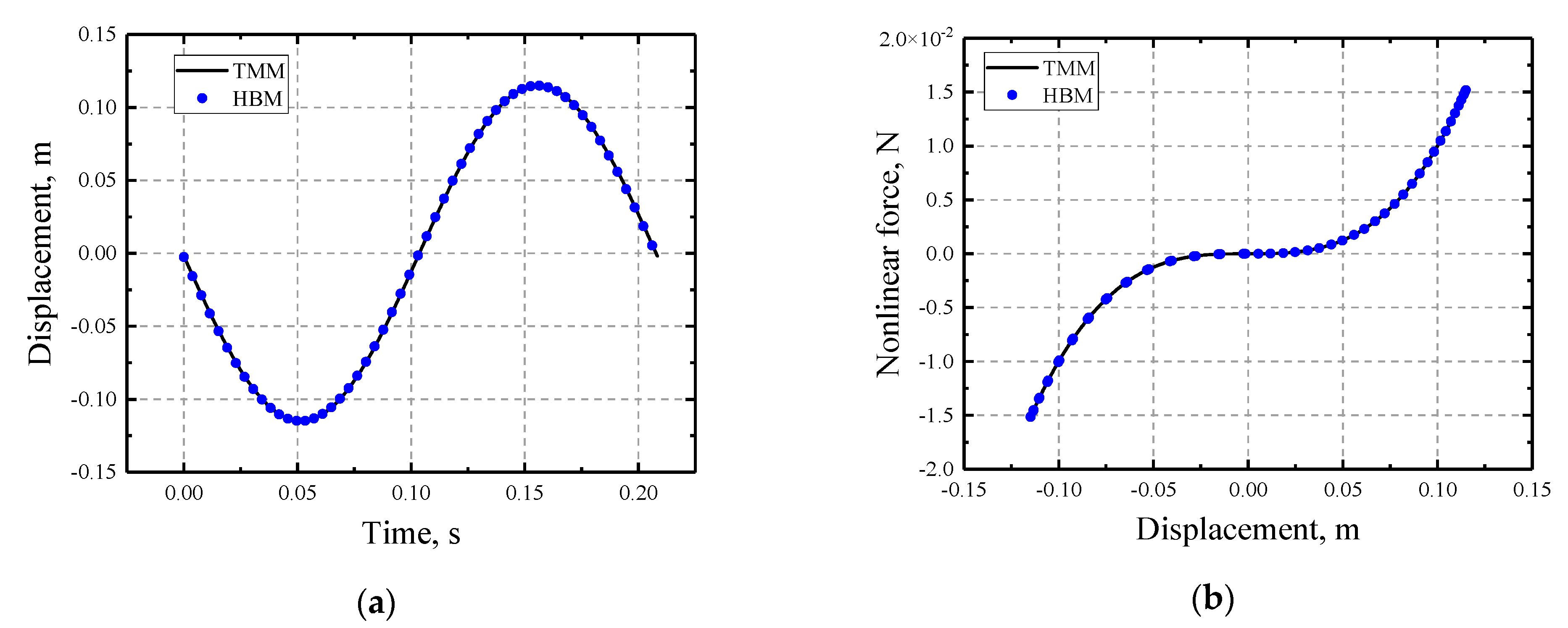
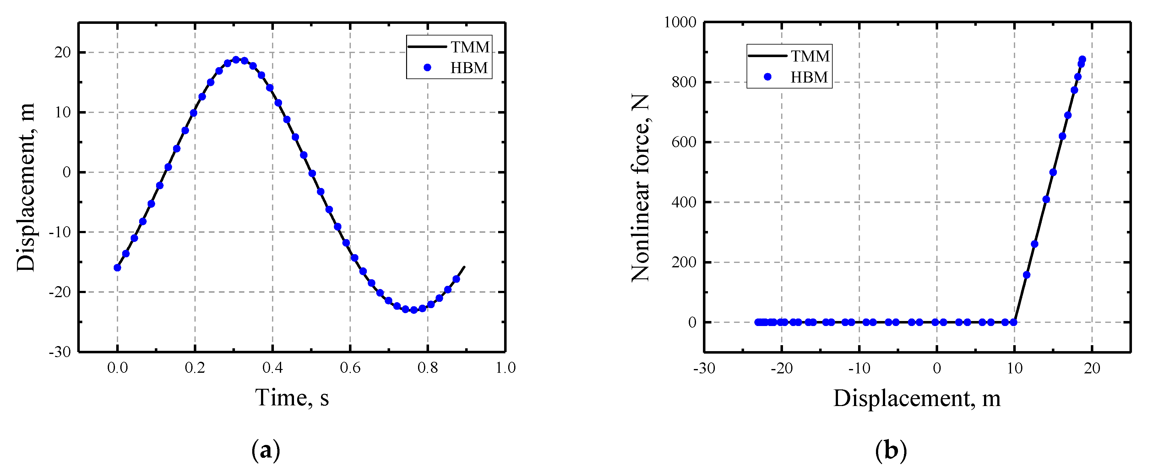
3.1.1. The Duffing Oscillator

A Duffing oscillator is utilized in this section, as shown in Figure 1, with stiffness coefficient k = 40 and damping coefficient c = 0.1$\sqrt{40}$ respectively. The nonlinear force is expressed in the form of cubic function, and the friction coefficient $k_{\tau }$ is the investigated parameter in sensitivity analysis.

Based on the model mentioned above, the equation of motion for this system takes the form:

$$m\ddot{x}+c\dot{x}+kx+f_{\tau }\left(x\right)+f_e=0$$

(33)

where the excitation force f_e has the form $f_e=-100\sin \left(\omega t\right)$. Although Equation (33) can be easily solved using time integral method such as New-Mark time integral methods, for the purpose of verification, it is still solved by the HBM mentioned in Section 2.1. The first 9 Harmonic components are kept and the number of time sampling points in Fourier transformation is 4096.

Firstly, the responses of the system with different friction coefficients are obtained. It can be seen in Figure 2 that multi-solution regions exist in the response curve. With increase of friction coefficients, the multi-solution regions grow larger and maximum amplitudes decrease. To verify the accuracy of HBM, time-domain displacement results obtained by the HBM and the time marching method (TMM) when k_τ = 100 N/m³ are illustrated in Figure 3 and Figure 4. The results show that high accuracy is achieved.

The sensitivity coefficients are specifically defined as the variation of maximum displacements when the parameters of interfaces change by one percent, as shown in Figure 5. Results reveal that with increase of friction coefficient, the sensitivity of the response will decrease. An abrupt change of first-order sensitivity happens at around ω = 6.5 rad/s. In this case, the first-order sensitivity is extremely sensitive to the variation of friction coefficient thus the values of second-order sensitivity rise, as shown in Figure 5b.

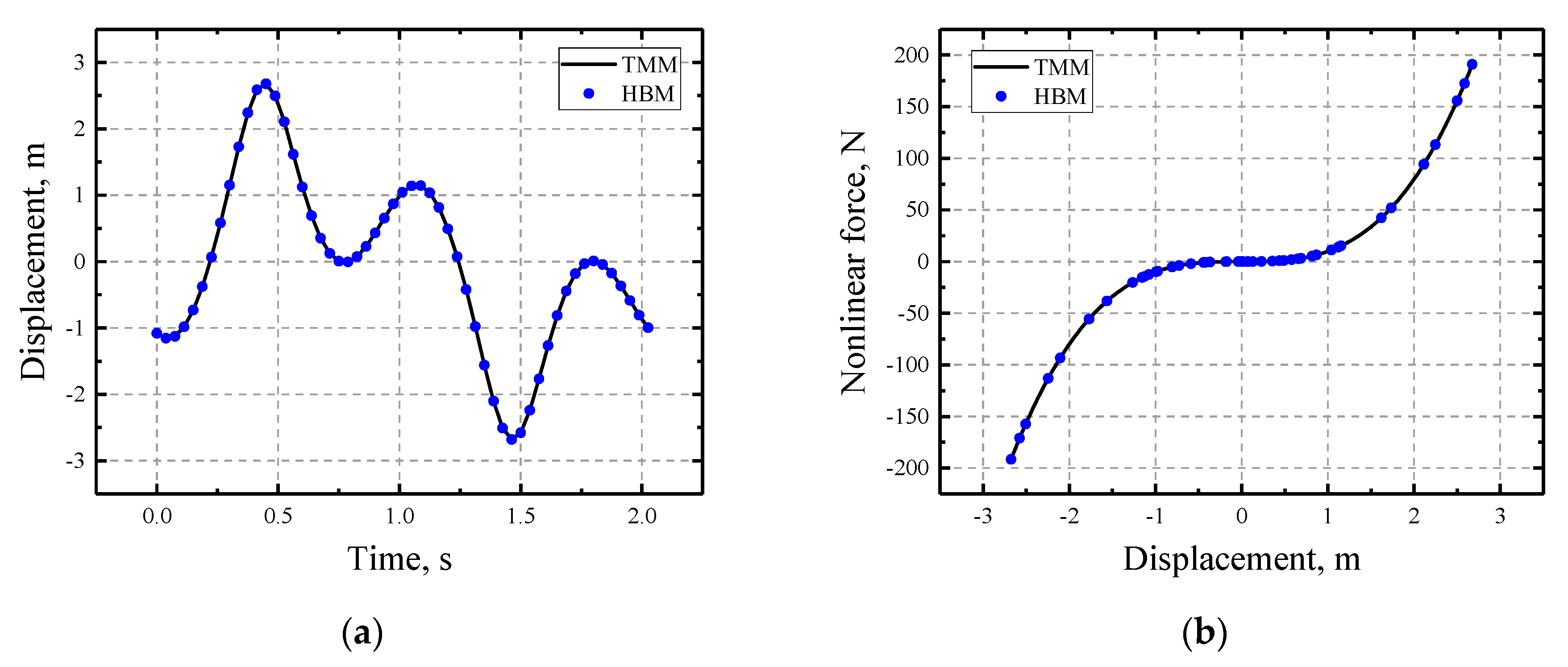
3.1.2. The Gap Model

As plotted in Figure 6, a similar oscillator subjected to pure-collision nonlinear force is applied in this section. Since no friction force is introduced in this system, it is referred to as the gap model.

The equation of motion for this model is exactly the same with Equation (33) while the nonlinear force has the following form:

$$f_{\tau }=\{\begin{array}{ccc}{k}_{\tau }\left(x-g\right)& & x\ge g\\ 0& & x<g\end{array}$$

(34)

where g is the prescribed clearance and k_y is the normal stiffness.

Figure 7 shows the response of the system with different normal stiffness and initial gaps. It can be seen that an offset of the critical speed exists in both cases. With the increase of normal stiffness or decrease of initial gap, the critical speed tends to increase. And multi-solution region emerges as a result. Results have been shown to be consistent with the work done by Petrov et al. [31]. Time-domain displacement results at ω = 7.029 rad/s obtained by the HBM and TMM are compared in Figure 8 and the accuracy of the HBM can be proved.

Moreover, the sensitivities of the response with respect to normal stiffness and initial gaps are obtained, as illustrated in Figure 9 and Figure 10. It can be seen that multi-solution regions also appear in the sensitivity curves. With an increase of normal stiffness, the multi-solution region tends to grow larger, as shown in Figure 9a. Moreover, with an increase of the initial gap, the sensitivities of the system increase and the multi-solution region shrinks, as illustrated in Figure 10a.

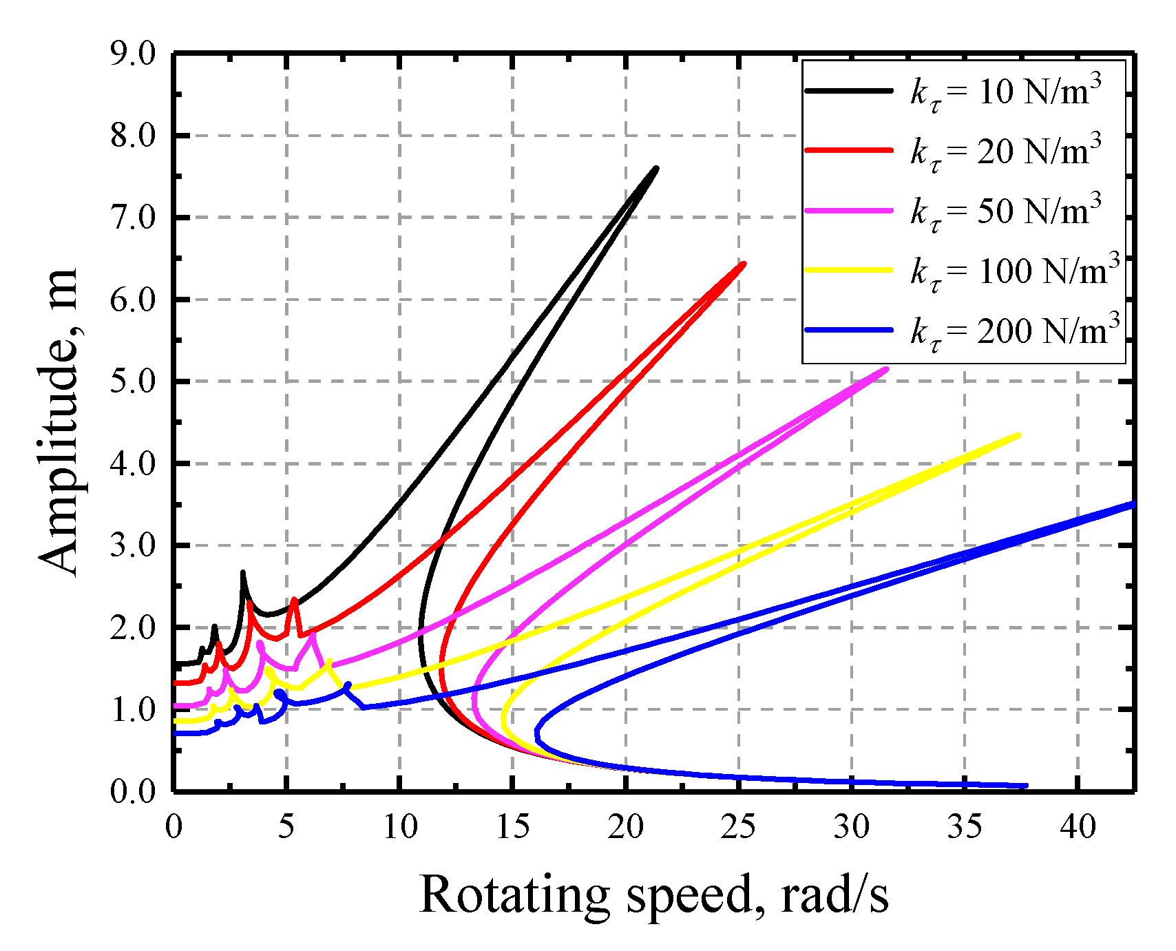
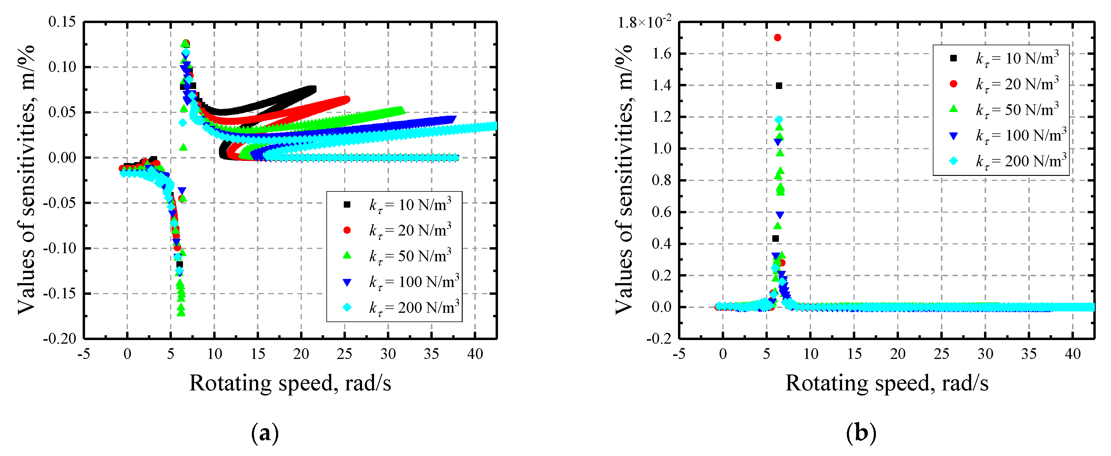
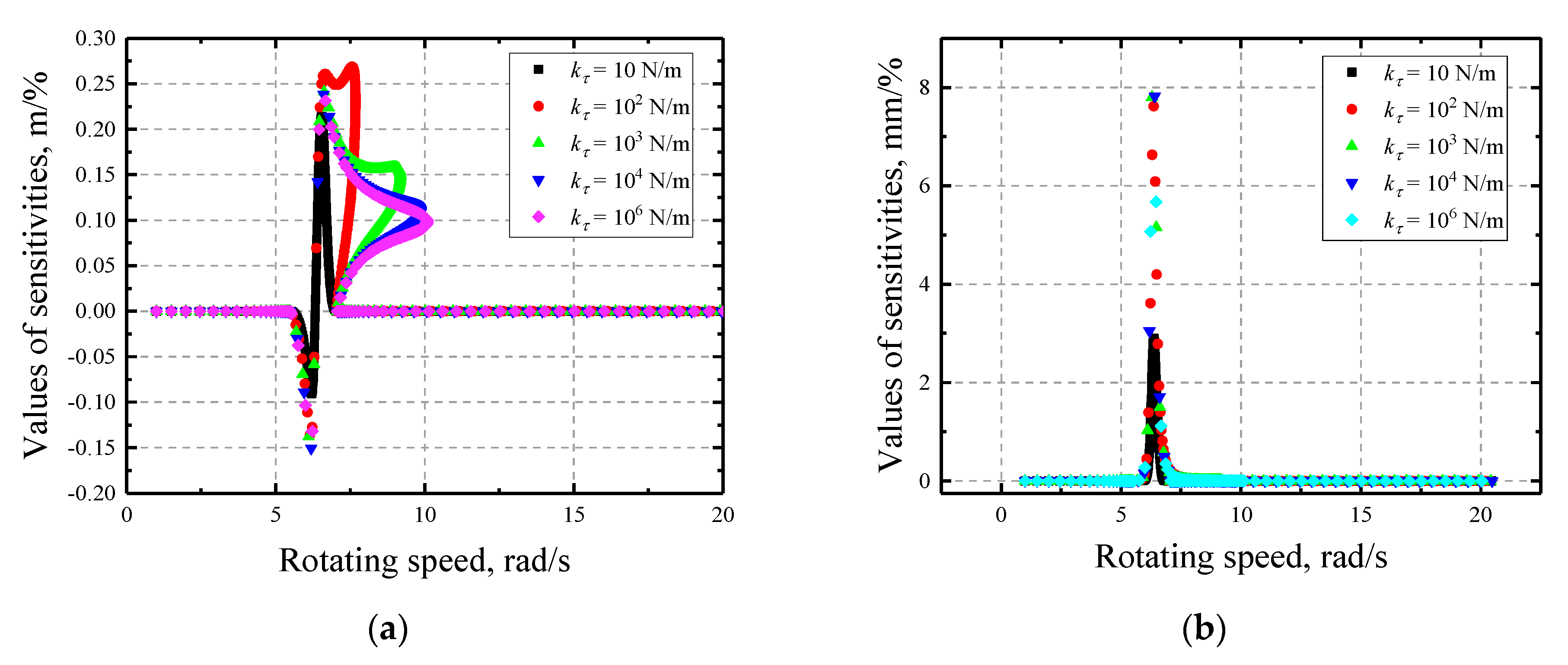
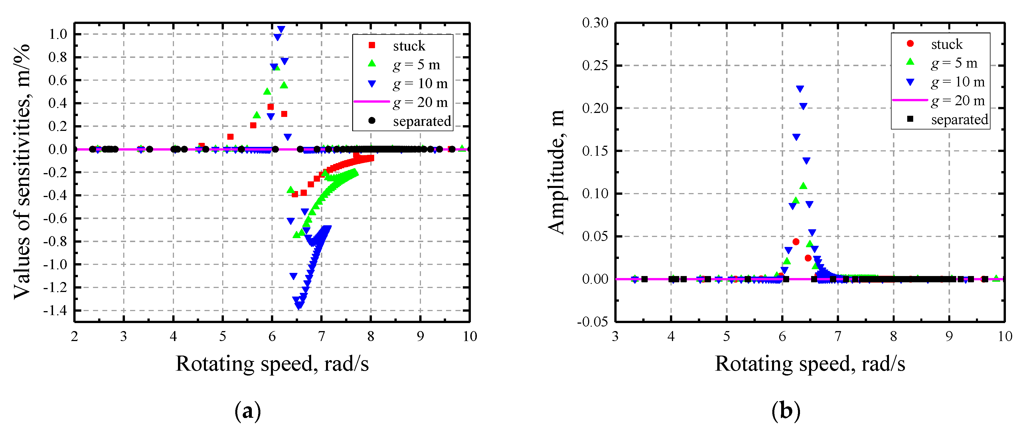
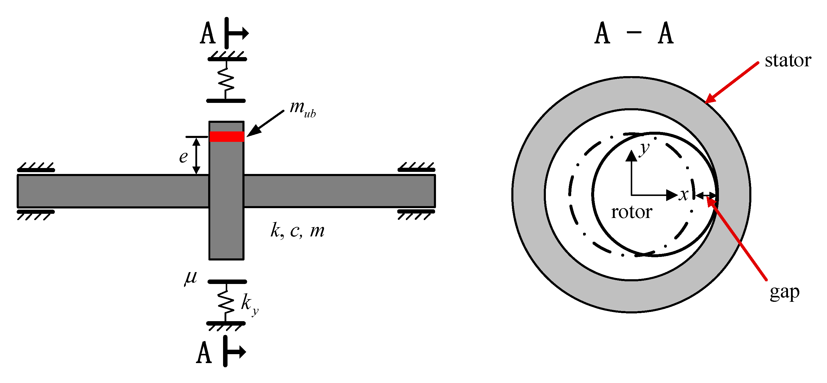
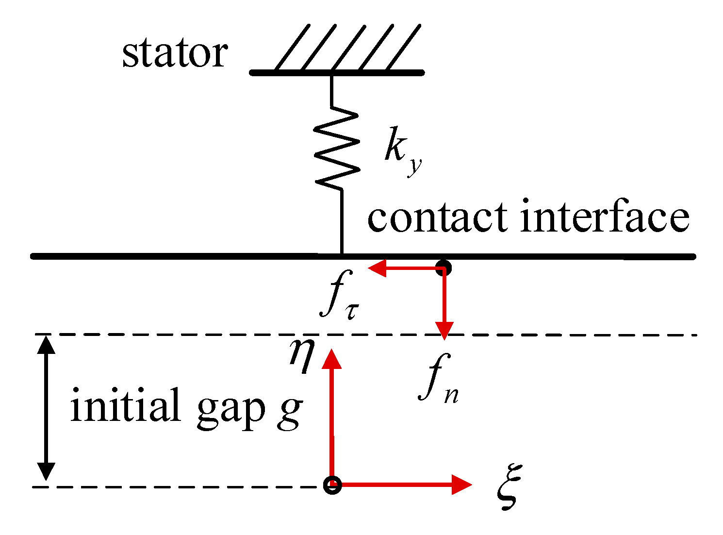
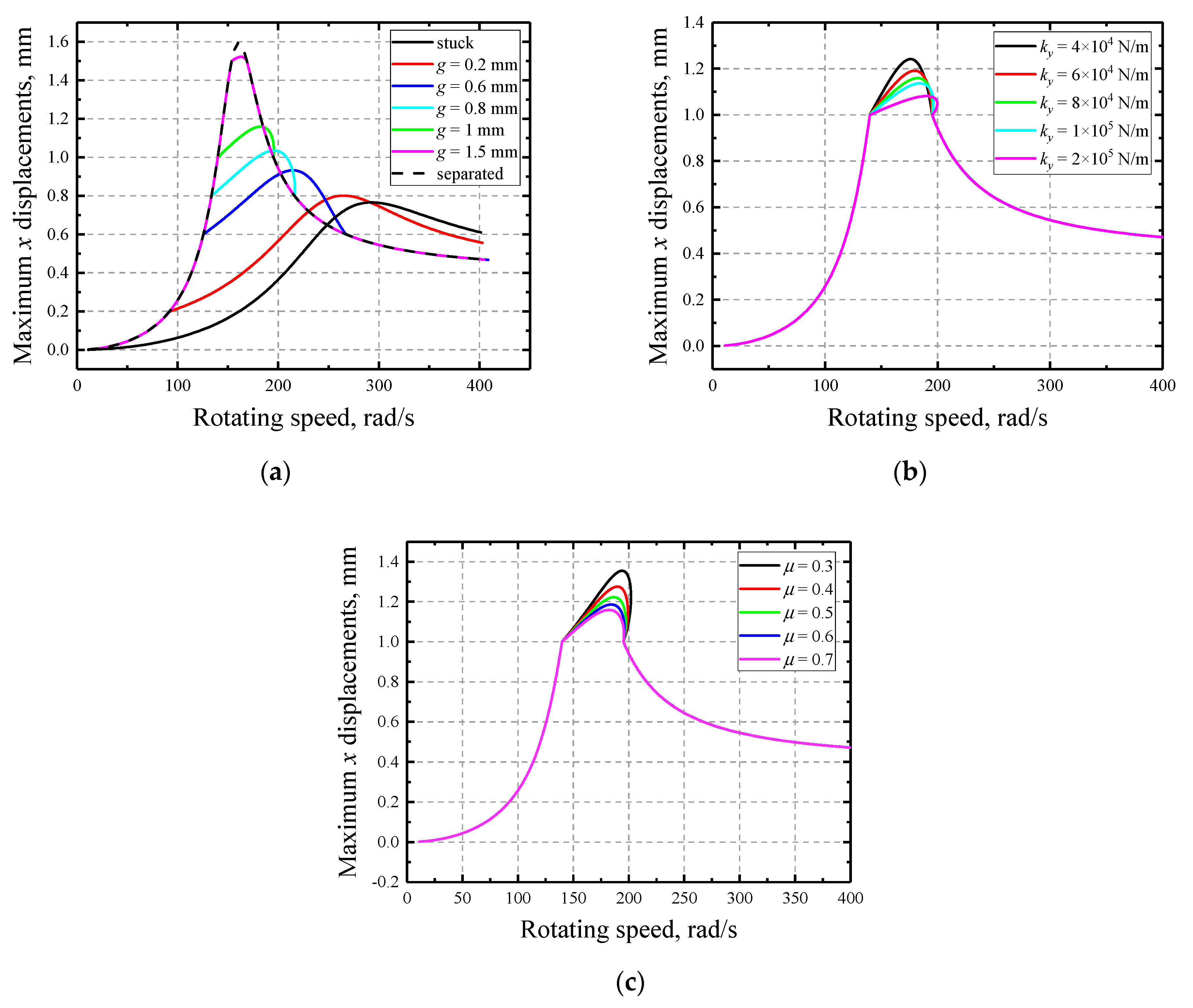
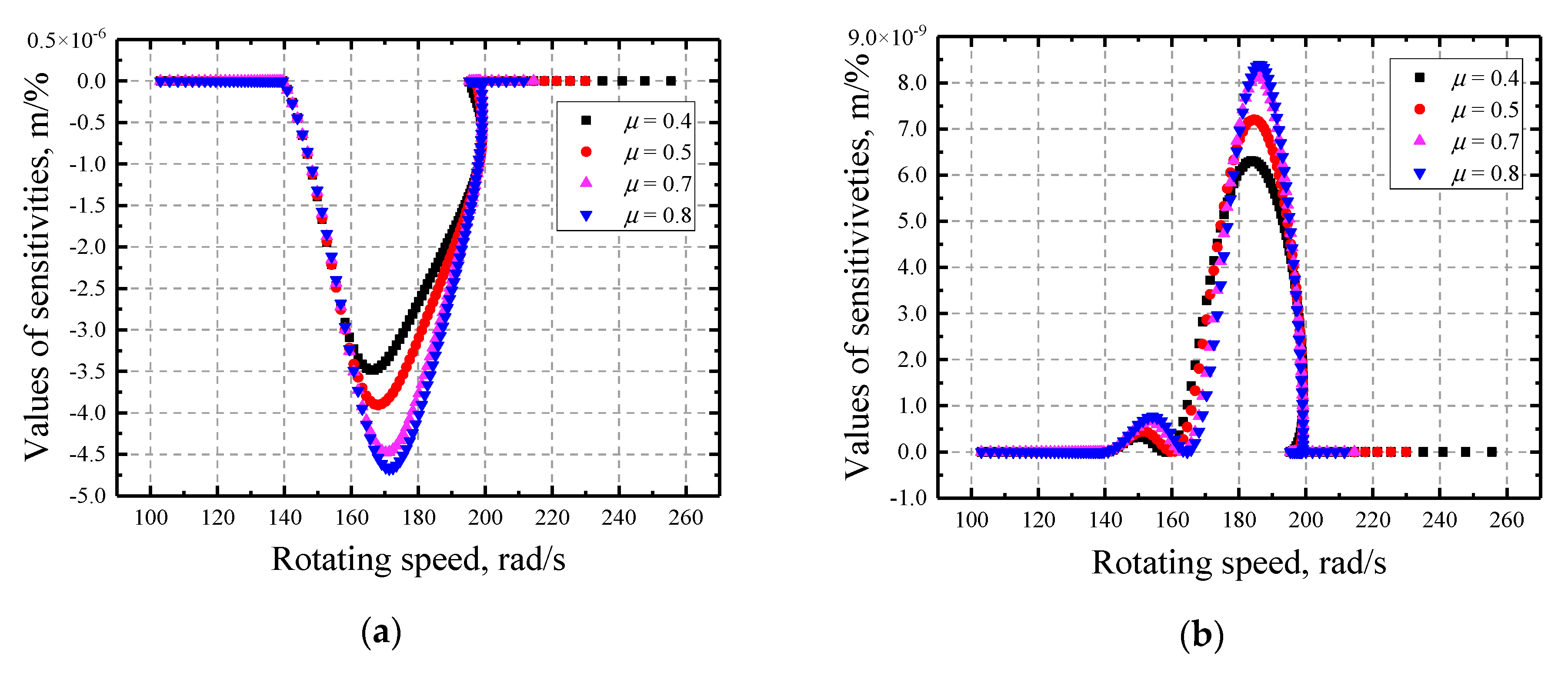
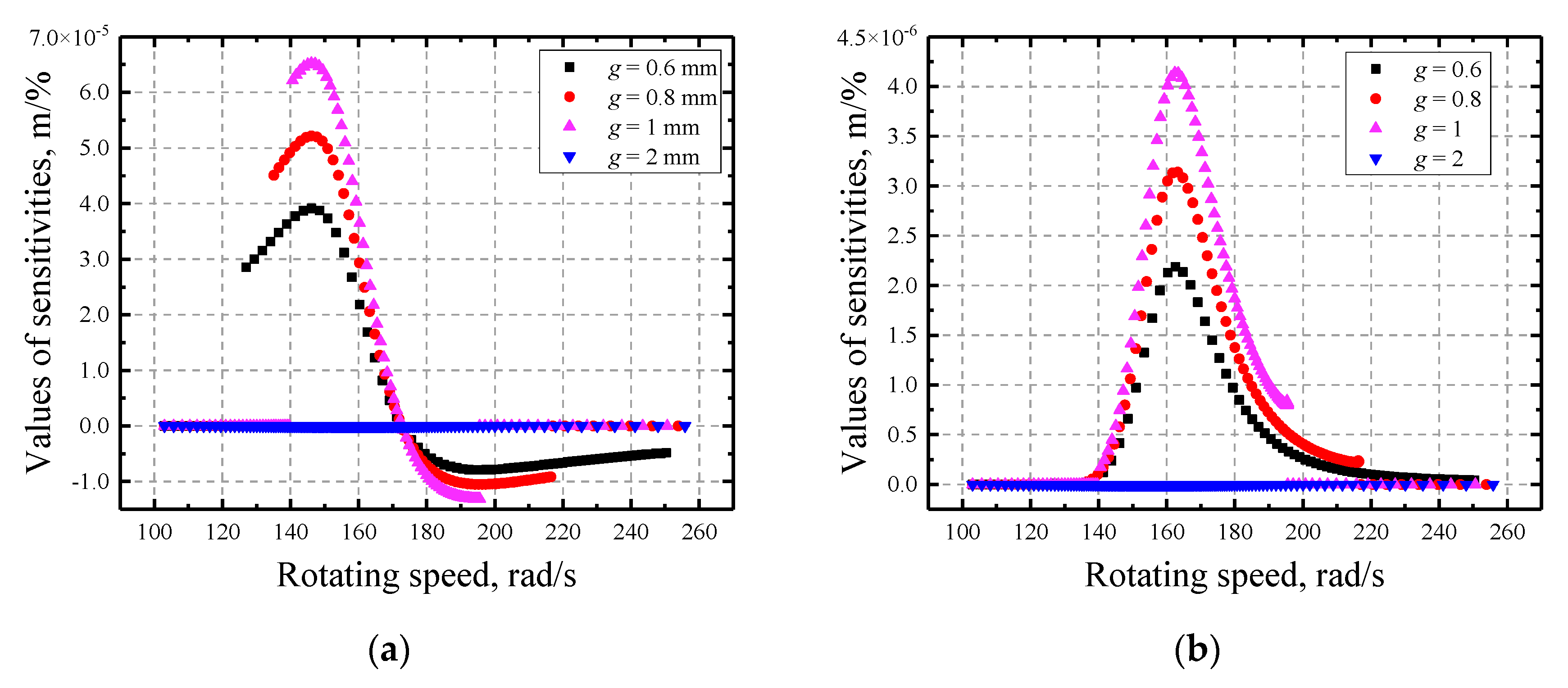
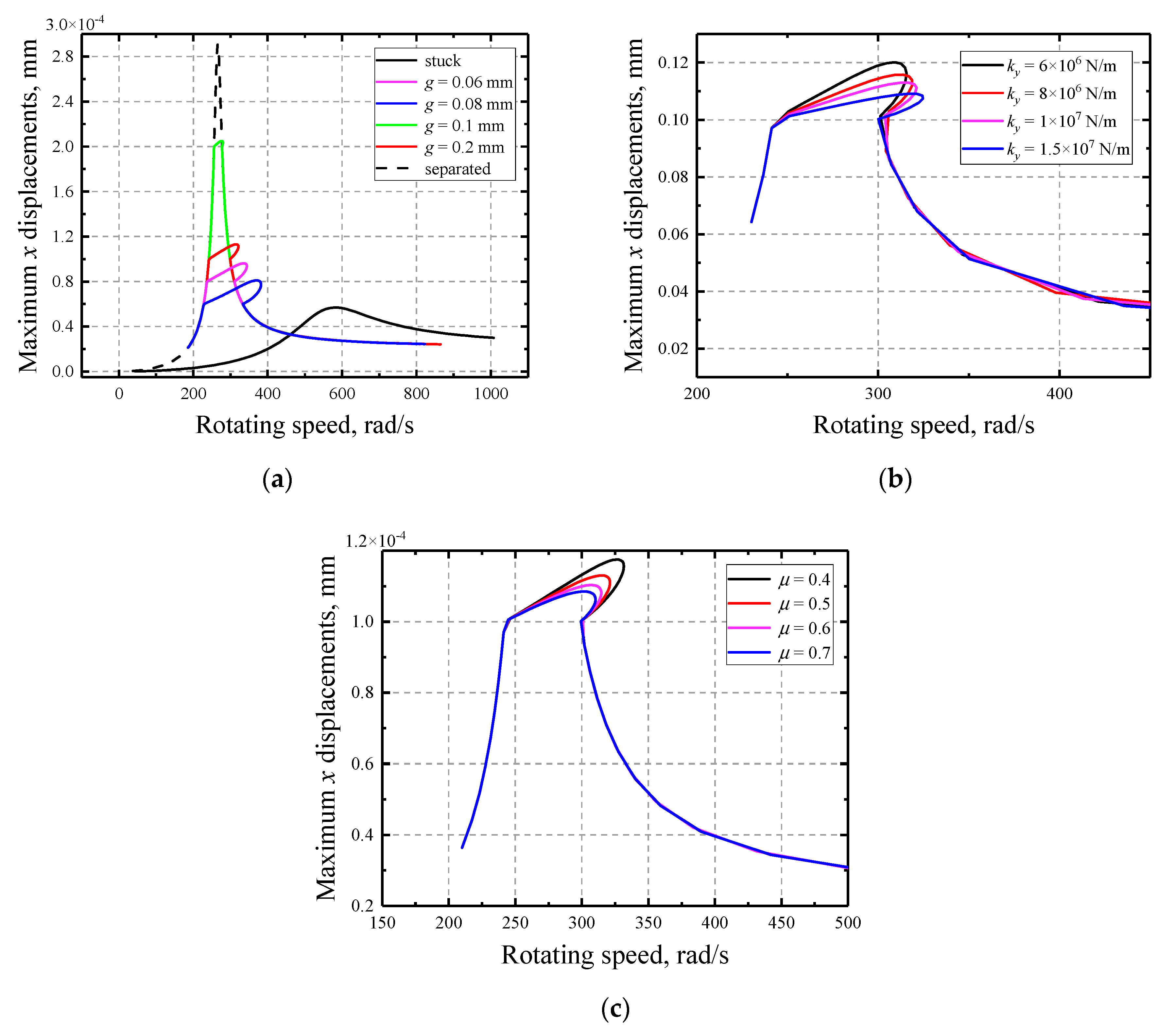
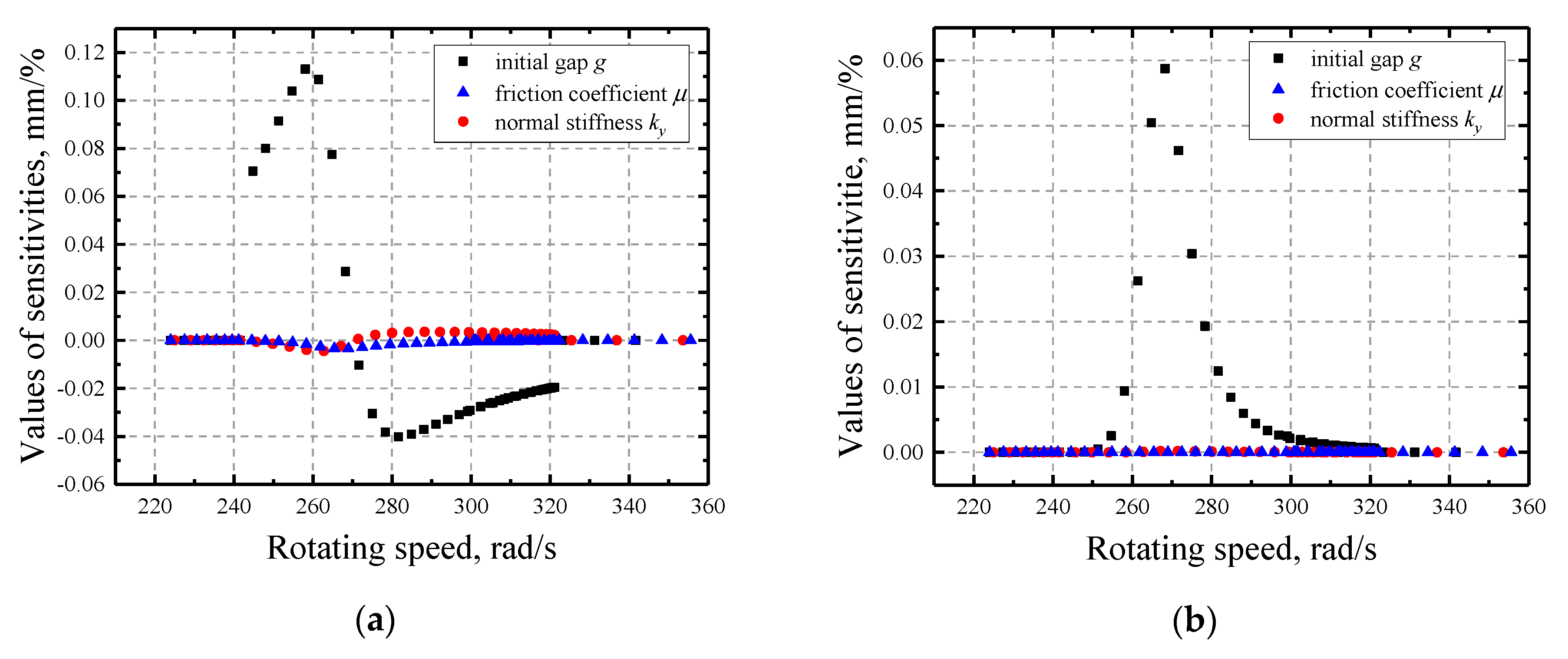
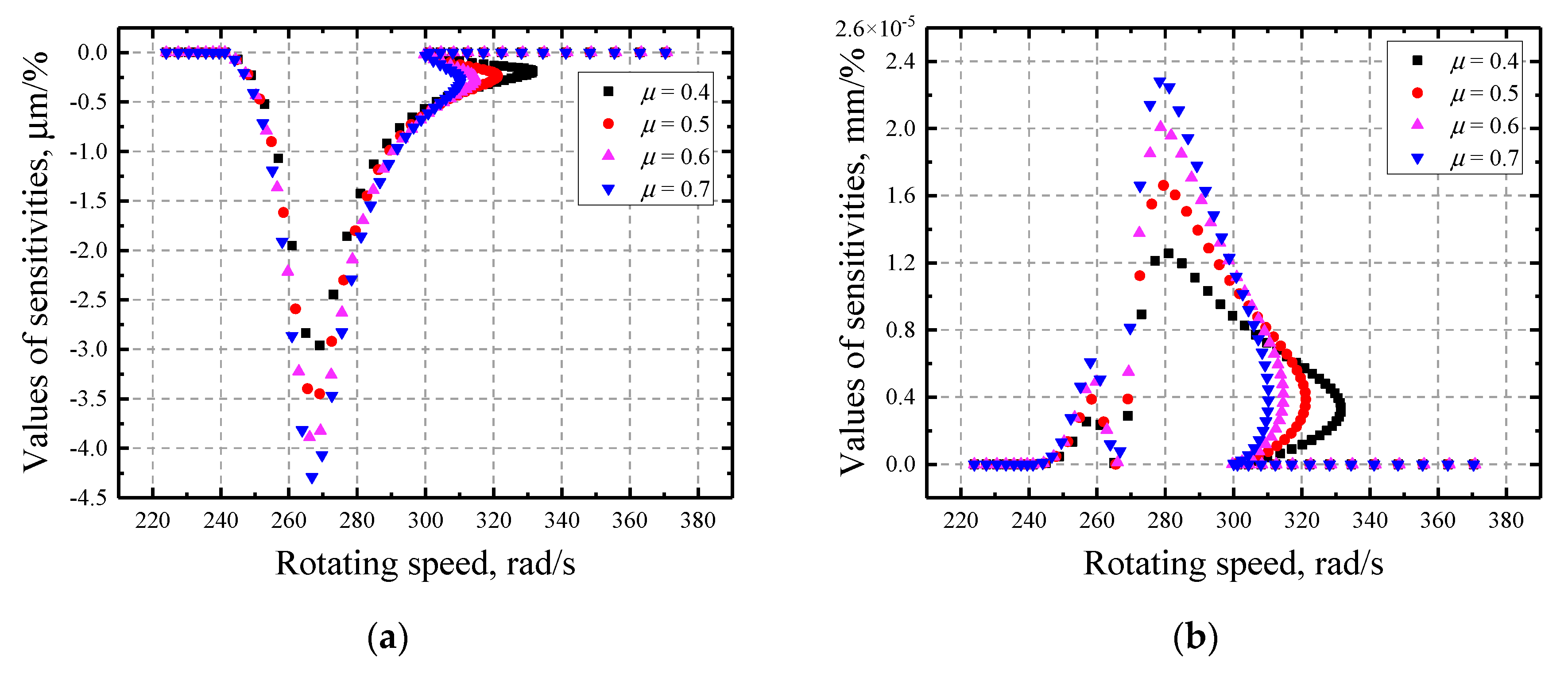
3.2. Sensitivity Analysisof a Jeffcott Rotor

Since the accuracy and capability of the methods adopted are demonstrated in Section 3.1, in this section the sensitivities of a rotor subjected to rubbing forces are investigated by adopting a lumped model, which is also named a Jeffcott rotor. A schematic diagram of the Jeffcott rotor is illustrated in Figure 11. It’s assumed that the periodic excitation force is induced by the unbalanced mass m_ub and the eccentric distance is e. The structural damping coefficient, c, is assumed to be proportional to the stiffness k and the mass m. And the relevant parameters are listed in

Table 1. Constant parameters of the Jeffcott rotor.

Parameter Name	Unit	Value
Eccentric distance e	mm	0.4
Stiffness k	N/m	5 × 104
Mass m	kg	2
Damping coefficient c	(N·s)/m	80

.

The influences of other parameters of rubbing interfaces, such as normal stiffness k_y and initial gap g, are investigated. The normal values of normal stiffness k_y, initial gap g and friction coefficient μ are 8 × 10⁴ N/m, 1 mm, and 0.7, respectively.

The friction model applied is a classical Coulomb friction model, as shown in Figure 12. It should be noted that the model is established based on local rotating frame. The analytical expressions for tangential rubbing force f_τ and normal rubbing force f_n in Figure 12 can be derived in time domain easily. As for f_n, since the values of force along normal direction will always be positive, it can be expressed by the following formula:

$$f_n=\{\begin{array}{ccc}0& & \eta <g\\ k_y\left(\eta -g\right)& & \eta \ge g\end{array}$$

(35)

Then the tangential friction force can also be determined in the following form:

$$f_{\tau }=\{\begin{array}{ccc}0& & f_n=0\\ -\mu f_n& & f_n>0\end{array}$$

(36)

where μ is the friction coefficient at the interfaces; f_τ is always negative considering that the direction of friction force is opposite to the direction of relative velocity.

Based on this friction model, firstly, the response of the Jeffcott rotor with different initial parameters of rubbing interfaces is illustrated. These parameters include the normal stiffness of stator, the friction coefficient and the initial gap. The first seven harmonic components are kept to approximate the periodic response.

Firstly, the sensitivity of the response to different parameters is investigated using the once-at-a-time (OAT) method [32], which implies changing an individual variable slightly to investigate its influence on the response. According to Figure 13a, the variation of initial gap g has a significant influence on the response curve of the Jeffcott rotor. It can not only influence the maximum displacements, but also determines the range of the speed region subjected to rubbing forces. Furthermore, with the increase of initial gap g, the influence of initial gap gradually becomes less significant since the variation of response curve becomes smaller. Although normal stiffness k_y and friction coefficient μ don’t influence the response as the way initial gap does, they can change the characteristics of multi-solution region. As shown in Figure 13b,c, with the decrease of k_y or increase of μ, the multi-solution region narrows. The influence of ky and μ is much smaller than that of the initial gap g, according to the variation of the response curve.

Figure 14 shows the sensitivity coefficients of the response, which is defined as the variation of maximum displacements when the parameters of rub interfaces change by one percent. In Figure 14a, first-order sensitivities with respect to all parameters of rub interfaces are equal to zero when the rotation speed range is outside of 138–195 rad/s. A similar phenomenon can be found in Figure 13a, where the response characteristics of the rotor can be regarded as a linear system outside the speed range 138–195 rad/s. The abrupt jump of the sensitivity curve with respect to initial gap g represents the change of contact/separation status. Among them the initial gap g plays a dominant role since it determines whether rub-impact exists and the results is consistent with that obtained by the OAT method. Similar phenomena also exist in the second-order sensitivity curves with the initial gap being the most significant impact factor, as illustrated in Figure 14b. It should be noted that first-order sensitivities are much larger than second-order sensitivities, so our discussions are mainly based on the former case.

In Figure 15, Figure 16 and Figure 17 results are shown for cases when normal values of parameters are varied. As illustrated in Figure 15a,b, the first-order sensitivities decrease while friction coefficients are rising. Moreover, an obvious offset of the sensitivities is also observed, which reflects the emergence of a multi-solution region. Figure 16 shows the results of sensitivities with different normal stiffness coefficients. The variation of sensitivities is relatively much smaller in this case, which implies that the response is relatively less sensitive to k_y. As is shown in Figure 17, the response becomes more sensitive with the increase of the initial gap and after it reaches a threshold the rotor becomes a linear system, as seen in the separated condition illustrated in Figure 13a.

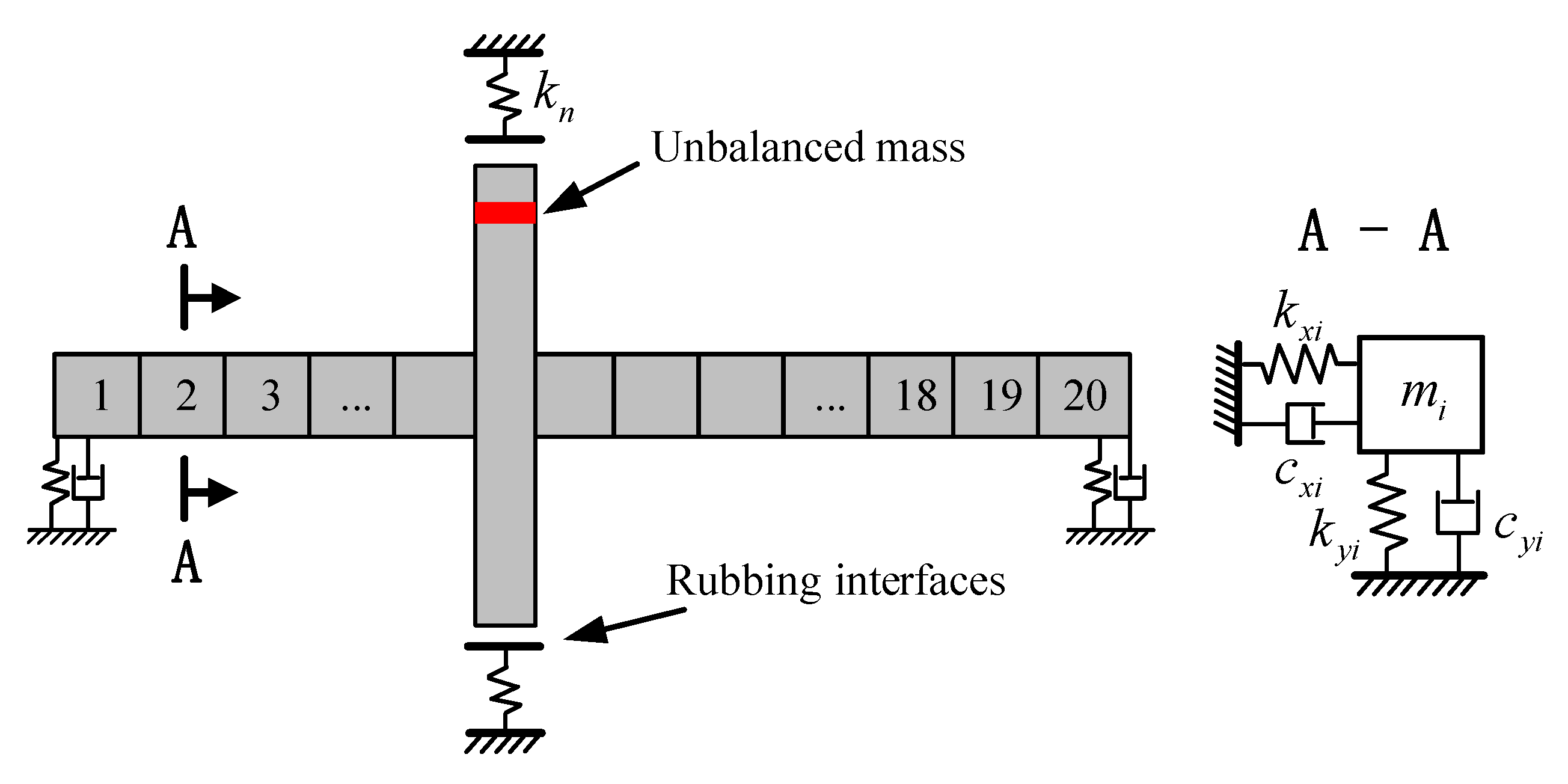
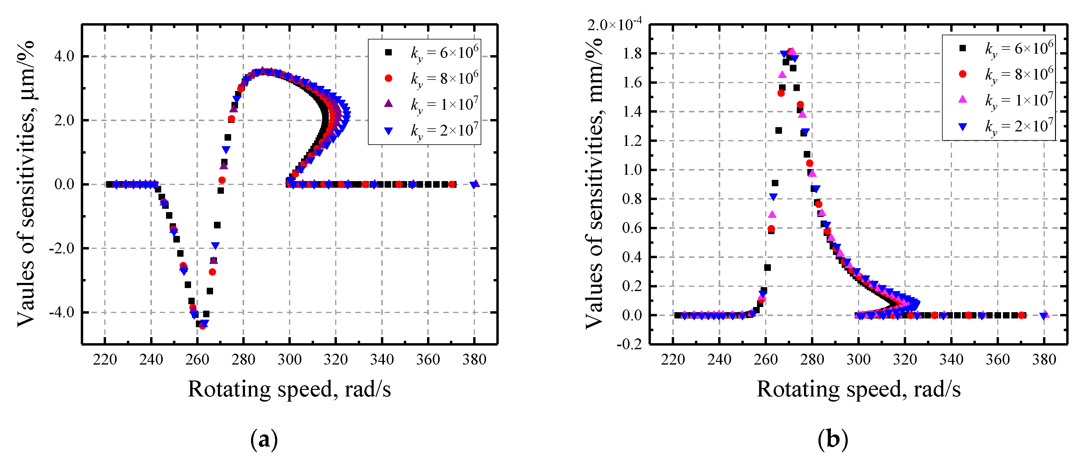
3.3. Sensitivity Analysis Based on Finite Element Model

Another rotor with rub-impact is discretized using the finite element method (FEM). As shown in Figure 18, the model is made up of 20 equal-length beam elements with the Young’s modulus, density and Poisson’s ratio equaling to 2 × 10⁵ MPa, 7.8 × 10³ kg/m³ and 0.3, respectively. The model is supported at both ends of the shaft. The motion of each element is assumed to be within the plane vertical to axial direction. The multiplication of unbalanced mass and its eccentric distance is equal to 7.0711 × 10⁻⁴ kg·m in this paper and the excitation force is applied based on it. Moreover, the rubbing forces are applied to node 7, with the Coulomb friction model mentioned in Section 3.2. The nominal values of parameters of rubbing interfaces are also prescribed, with stator stiffness k_y, the friction coefficient μ and the initial gap g equal to 1.0 × 10⁷ N/m, 0.5, 0.1 mm, respectively. For the purpose of performance and accuracy, the time sampling number is 1024 and the first seven harmonic components are kept to approximate the response. The friction model applied on elements subjected to rubbing forces is exactly the same as that of Section 3.2.

Similar conclusions can be drawn based on this model, i.e., the response is much more sensitive to the initial gap g and with its increase the sensitivity decreases, as in Figure 19a. Outside of the speed range 260.9 rad/s to 298.9 rad/s there is no rub-impact forces so the response is exactly the same with that of separation status. When rubbing forces exist, a multi-solution region emerges because of the nonlinearity of the system. Moreover, the increase of normal stiffness and decrease of friction coefficient results in the expansion of the multi-solution region, as seen in Figure 19b,c.

Figure 20 shows the sensitivities of the frequency-domain response to different parameters of rub-impact interfaces. Similar phenomena have been observed as obtained by the Jeffcott rotor. The responses are more sensitive to the initial gap g compared to the other investigated parameters. The sensitivity curve near the vicinity of the rotating speeds where the separation-contact status transformation happens is discontinuous, since the sensitivities are equal to zero when no rub-impact exists. An obvious offset of sensitivities is seen under this condition, as a result of the existence of a multi-solution region in the response curve.

By changing initial values of initial gap g, the sensitivities to the initial gap with different prescribed g values are investigated, as shown in Figure 21. Still, s discontinuity exists where separation-contact transformation happens. With the increase of initial gap g, the speed region subjected to rub-impact narrows and the response becomes more sensitive. Moreover, with an increase of the initial gap, the multi-solution region of sensitivities narrows as well.

Similarly, as seen in Figure 22, results show that with decrease of friction coefficient the offset of sensitivities, which is more obvious in the 300–330 rad/s speed range when μ is equal to 0.4, becomes more severe with the decrease of friction coefficients. In other words, the multi-solution region grows while μ is decreasing. This is consistent with the results obtained by the OAT method, as illustrated in Figure 19c.

According to Figure 23, the variation of normal stiffness k_y may also change the stable sensitivity region. Moreover, the variation of k_y has relatively little influence on the sensitivities, but the multi-solution region develops indeed with the increase of k_y.

4. Conclusions

This paper investigated the sensitivity characteristics of rotors subjected to rub-impact problems to parameters of rubbing interfaces. The harmonic balance method and pseudo arc-length continuation method are utilized to obtain the steady-state response of the system. Furthermore, the analytical expressions for the sensitivity coefficients are derived for the purpose of accuracy and performance. Two classical models, namely the Duffing oscillator and the gap model, are utilized to verify the accuracies and capabilities of the adopted methods. Then numerical investigations of the sensitivities of steady-state response to parameters of rubbing interfaces are performed and conclusions are drawn as follows:

(1)

The response of rotors subjected to rub-impact is sensitive to the parameters of rub interfaces only when the amplitudes are large enough to reach or exceed the prescribed initial clearance. If that is not the case, the whole system is equal to a linear system under a periodical excitation force.

(2)

The response of the rotor is much more sensitive to the initial gap with the two other factors being relatively insignificant. The sensitivities to the initial gap g are not contiguous at rotating speeds where a separation/contact status transformation happens since it determines the existence of rub-impact.

(3)

With the increase of initial gap, the rotors become more sensitive. In contrast, the friction coefficient has negative impact on the sensitivities and the multi-solution region grows larger with its decrease. Moreover, the variation of normal stiffness has relatively little influence on the sensitivities but it does influence the characteristics of the multi-solution region, i.e., the region expands as it increases.

References

1. Fan, Y.; Wang, S.; Yang, Z. Stability Margin Sensitivity Analysis of a Multi-Rotor System Geared by Spiral Bevel Gear pairs. Manuf. Sci. Eng. 2010, 97, 3215–3218. [Google Scholar] [CrossRef]
2. Kim, J.; Sim, W.; Chung, J. Modal characteristics and dynamic stability of a whirling rotor with flexible blades. Appl. Math. Model. 2021, 89, 1–18. [Google Scholar] [CrossRef]
3. Zhang, Y.-M.; Liu, Q.-L.; Li, H.; Wen, B.-C. Reliability sensitivity investigation of impact-rub for rotor-stator systems. J. Mol. Endocrinol. 2006, 21, 848–853. [Google Scholar] [CrossRef] [Green Version]
4. Ritto, T.G.; Lopez, R.H.; Sampaio, R.; de Cursi, J.E.S. Robust optimization of a flexible rotor-bearing system using the Campbell diagram. Eng. Optimiz. 2011, 43, 77–96. [Google Scholar] [CrossRef]
5. Helton, J.C.; Johnson, J.D.; Sallaberry, C.J.; Storlie, C.B. Survey of sampling-based methods for uncertainty and sensitivity analysis. Reliab. Eng. Syst. Saf. 2006, 91, 1175–1209. [Google Scholar] [CrossRef] [Green Version]
6. Zhang, J.; TerMaath, S.; Shields, M.D. Imprecise global sensitivity analysis using bayesian multimodel inference and importance sampling. Mech. Syst. Signal Process. 2021, 148, 107162. [Google Scholar] [CrossRef]
7. Changqing, S.U.; Yimin, Z.; Chunmei, L.V.; Hui, M.A. Natural frequency reliability sensitivity analysis of a rotor system. J. Vib. Shock. 2009, 28, 56–59. [Google Scholar] [CrossRef]
8. Melchers, R.E.; Ahammed, M. A fast approximate method for parameter sensitivity estimation in Monte Carlo structural reliability. Comput. Struct. 2004, 82, 55–61. [Google Scholar] [CrossRef]
9. Lataillade, A.D.; Blanco, S.; Clergent, Y.; Dufresne, J.L.; Hafi, M.E.; Fournier, R. Monte Carlo method and sensitivity estimations. J. Quant. Spectrosc. Radiat. Transf. 2018, 75, 529–538. [Google Scholar] [CrossRef] [Green Version]
10. Petrov, E.P. Sensitivity analysis of nonlinear forced response for bladed discs with friction contact interfaces. In Proceedings of the Asme Turbo Expo 2005, Reno, NV, USA, 6–9 June 2005; Volume 4, pp. 483–494. [Google Scholar] [CrossRef]
11. Petrov, E.P. Analysis of sensitivity and robustness of forced response for nonlinear dynamic structures. Mech. Syst. Signal Process. 2009, 23, 68–86. [Google Scholar] [CrossRef]
12. Leister, T.; Baum, C.; Seemann, W. Sensitivity of computational rotor dynamics towards the empirically estimated lubrication gap clearance of foil air journal bearings. Proc. Appl. Math. Mech. 2016, 16, 285–286. [Google Scholar] [CrossRef]
13. Yan, S.; Sievert, R. Vibration Sensitivity of Large Turbine Generator Shaft Trains to Unbalance. In Proceedings of the 9th IFToMM International Conference on Rotor Dynamics, Cham, Switzerland, 22–25 September 2015; pp. 3–14. [Google Scholar]
14. Pan, H.; Yuan, H.; Zhao, T.; Yang, W. Sensitivity Analysis of Wheel Quality and Location on Rotor Critical Speed. J. Vib. Meas. Diagn. 2017, 37, 532–538. [Google Scholar] [CrossRef]
15. Papini, L.; Gerada, C. Sensitivity Analysis of Rotor Parameters in Solid Rotor Induction Machine. In Proceedings of the IEEE International Electric Machines and Drives Conference, Miami, FL, USA, 21–24 May 2017. [Google Scholar]
16. Ying, G.; Wu, W.; Liu, S.; Zheng, S. Research on Bearing Load Sensitivity for Multi-support Rotor System. Zhejiang Electr. Power 2017, 36, 39–42. [Google Scholar] [CrossRef]
17. Anusonti-Inthra, P.; Corle, E.; Smith, B.; Nieto, Z. Sensitivity Analysis and Uncertainty Quantification of a Coaxial Rotor System. In Proceedings of the AIAA Aviation 2019 Forum, Dallas, TX, USA, 17–21 June 2019; p. 15. [Google Scholar]
18. Choy, F.K.; Padovan, J. Non-linear transient analysis of rotor-casing rub events. J. Sound Vib. 1987, 113, 529–545. [Google Scholar] [CrossRef]
19. Dai, X.; Zhang, X.; Jin, X. The partial and full rubbing of a flywheel rotor-bearing-stop system. Int. J. Mech. Sci. 2001, 43, 505–519. [Google Scholar] [CrossRef]
20. Feng, Z.C.; Zhang, X.Z. Rubbing phenomena in rotor-stator contact. Chaos Solitons Fractals 2002, 14, 257–267. [Google Scholar] [CrossRef]
21. Patel, T.H.; Darpe, A.K. Vibration response of a cracked rotor in presence of rotor-stator rub. J. Sound Vib. 2008, 317, 841–865. [Google Scholar] [CrossRef]
22. Popprath, S.; Ecker, H. Nonlinear dynamics of a rotor contacting an elastically suspended stator. J. Sound Vib. 2007, 308, 767–784. [Google Scholar] [CrossRef]
23. Liu, G.-Z.; Chen, Y.-Z.; Liu, Y.; Wen, B.-C. Experimental investigation of rotor rubbing faults. Adv. Mater. Res. 2012, 490, 1048–1052. [Google Scholar] [CrossRef]
24. Ma, H.; Tai, X.; Zhang, Z.; Wen, B. Dynamic Characteristic Analysis of a Rotor System with Rub-impact Fault Considering Rotor-stator Misalignment. Prz. Elektrotechniczny 2012, 88, 145–149. [Google Scholar]
25. Shen, X.; Jia, J.; Zhao, M. Effect of parameters on the rubbing condition of an unbalanced rotor system with initial permanent deflection. Arch. Appl. Mech. 2007, 77, 883–892. [Google Scholar] [CrossRef]
26. Yao, H.; Han, Q.; Li, L.; Wen, B. Method for Detecting Rubbing Fault in Rotor System Based on Harmonic Components. J. Mech. Eng. 2012, 48, 43–48. [Google Scholar] [CrossRef]
27. Behzad, M.; Alvandi, M. Friction-induced backward rub of rotors in non-annular clearances: Experimental observations and numerical analysis. Tribol. Int. 2020, 152. [Google Scholar] [CrossRef]
28. Liu, Y.; Li, J.T.; Feng, K.P.; Zhao, Y.L.; Yan, X.X.; Ma, H. A novel fault diagnosis method for rotor rub-impact based on nonlinear output frequency response functions and stochastic resonance. J. Sound Vib. 2020, 481, 17. [Google Scholar] [CrossRef]
29. Zhang, Y.; Wen, B.; Liu, Q. Sensitivity Analysis for Rotor Systems with Impact-rub. Mach. Des. Res. 2002, 18, 28–29. [Google Scholar] [CrossRef]
30. Yin, Y.; Di, Y.; Yao, Z. Arc-length Continuation Algorithm for Nonlinear Finite Element Equations. Acta Sci. Nat. Univ. Pekin. 2017, 53, 793–800. [Google Scholar] [CrossRef]
31. Petrov, E.P.; Ewins, D.J. Analytical formulation of friction interface elements for analysis of nonlinear multi-harmonic vibrations of bladed disks. J. Turbomach. Trans. ASME 2003, 125, 364–371. [Google Scholar] [CrossRef]
32. Borgonovo, E.; Plischke, E. Sensitivity analysis: A review of recent advances. Eur. J. Oper. Res. 2015, 248, 869–887. [Google Scholar] [CrossRef]
Figure 1. Sketch of the Duffing oscillator used for verification.
Applsci 11 01307 g001
Figure 2. Response curves of the Duffing oscillator with different friction coefficients.
Applsci 11 01307 g002
Figure 3. Response curve and hysteresis loop of the Duffing oscillator obtained by HBM and TMM at ω = 30.1612 rad/s and kτ = 10 N/m3: (a) The response curve; (b) The hysteresis loop.
Applsci 11 01307 g003
Figure 4. Response curve and hysteresis loop of the Duffing oscillator obtained by HBM and TMM at ω = 3.0672 rad/s and kτ = 10 N/m3: (a) The response curve; (b) The hysteresis loop.
Applsci 11 01307 g004
Figure 5. Sensitivities of the response of the Duffing oscillator to friction coefficient with different nominal values of friction coefficients: (a) First-order sensitivity; (b) Second-order sensitivity.
Applsci 11 01307 g005
Figure 6. The gap model subjected to pure-collision nonlinear force.
Applsci 11 01307 g006
Figure 7. Response curves of the gap model with different normal stiffness and initial clearances: (a) Response curves of the system at g = 10 m; (b) Response curves of the system at ky = 100 N/m.
Applsci 11 01307 g007
Figure 8. Response curve and hysteresis loop of the gap model obtained by HBM and TMM at ω = 7.029 rad/s, g = 10 m and ky = 100 N/m: (a) The response curve; (b) The hysteresis loop.
Applsci 11 01307 g008
Figure 9. Sensitivities of the response curve of the gap model to normal stiffness at g = 10 m: (a) First-order sensitivities; (b) Second-order sensitivities.
Applsci 11 01307 g009
Figure 10. Sensitivities of the response curve of the gap model to initial gaps at ky = 100 N/m: (a) First-order sensitivities; (b) Second-order sensitivities.
Applsci 11 01307 g010
Figure 11. Schematic diagram of the Jeffcott rotor.
Applsci 11 01307 g011
Figure 12. The Coulomb friction model in local frame.
Applsci 11 01307 g012
Figure 13. The x-direction response curve of the Jeffcott rotor with different nominal values of the investigated parameters: (a) Response curves with different initial gaps at ky = 8 × 10⁴ N/m and μ = 0.7; (b) Response curves with different normal stiffness at g = 1 mm and μ = 0.7; (c) Response curves with different normal friction coefficients at ky = 8 × 10⁴ N/m and g = 1 mm.
Applsci 11 01307 g013
Figure 14. The sensitivity curves of the x-direction response of the Jeffcott rotor with respect to the three investigated parameters of rub interfaces at ky = 8 × 10⁴ N/m, μ = 0.7 and g = 1 mm: (a) First-order sensitivities; (b) Second-order sensitivities.
Applsci 11 01307 g014
Figure 15. The sensitivity curves of the response of the Jeffcott rotor with respect to friction coefficients at g = 1 mm and ky = 8 × 10⁴ N/m: (a) First-order sensitivities; (b) Second-order sensitivities.
Applsci 11 01307 g015
Figure 16. The sensitivity curves of the response of the Jeffcott rotor with respect to normal stiffness at g = 1 mm and μ = 0.7: (a) First-order sensitivities; (b) Second-order sensitivities.
Applsci 11 01307 g016
Figure 17. The sensitivity curves of the response of the Jeffcott rotor with respect to initial gaps at ky = 8 × 10⁴ N/m and μ = 0.7: (a) First-order sensitivities; (b) Second-order sensitivities.
Applsci 11 01307 g017
Figure 18. Sketch of the investigated finite element model.
Applsci 11 01307 g018
Figure 19. The x-direction response curve of the finite element model with different nominal values of the investigated parameters: (a) Response curves with different initial gaps at ky = 1 × 10⁷ N/m and μ = 0.5; (b) Response curves with different normal stiffness at g = 0.1 mm and μ = 0.5; (c) Response curves with different normal friction coefficients at ky = 1 × 10⁷ N/m and g = 0.1 mm.
Applsci 11 01307 g019
Figure 20. The sensitivity curves of the x-direction response of the finite element model with respect to the three investigated parameters of rub interfaces at ky = 1 × 10⁷ N/m, μ = 0.5 and g = 0.1 mm: (a) First-order sensitivities; (b) Second-order sensitivities.
Applsci 11 01307 g020
Figure 21. The sensitivity curves of the response of the finite element model with respect to initial gaps at μ = 0.5 and ky = 1 × 10⁷ N/m: (a) First-order sensitivities; (b) Second-order sensitivities.
Applsci 11 01307 g021
Figure 22. The sensitivity curves of the response of the Jeffcott rotor with respect to friction coefficients at g = 0.1 mm and ky = 1 × 10⁷ N/m: (a) First-order sensitivities; (b) Second-order sensitivities.
Applsci 11 01307 g022
Figure 23. The sensitivity curves of the response of the Jeffcott rotor with respect to normal stiffness at g = 0.1 mm and μ = 0.5: (a) First-order sensitivities; (b) Second-order sensitivities.
Applsci 11 01307 g023