Abstract
This paper has resulted from a continued study of spacecraft material degradation and space debris formation. The design and implementation of a thermal vacuum cycling cryogenic facility for the evaluation of space debris generation at a low Earth orbit (LEO) is presented. The facility used for spacecraft external material evaluation is described, and some of the obtained results are presented. The infrastructure was developed in the framework of a study for the European Space Agency (ESA). The main purpose of the cryogenic facility is to simulate the LEO spacecraft environment, namely thermal cycling and vacuum ultraviolet (VUV) irradiation to simulate the spacecraft material degradation and the generation of space debris. In a previous work, some results under LEO test conditions showed the effectiveness of the cryogenic facility for material evaluation, namely: the degradation of satellite paints with a change in their thermo-optical properties, leading to the emission of cover flakes; the degradation of the pressure-sensitive adhesive (PSA) used to glue Velcro’s to the spacecraft, and to glue multilayer insulation (MLI) to the spacecraft’s. The paint flakes generated are space debris. Hence, in a scenario of space missions where a spacecraft has lost the thermal shielding capability, the failure of PSA tape and the loss of Velcro properties may contribute to the release of the full MLI blanket, contributing to the generation of space debris that presents a growing threat to space missions in the main Earth orbits.
1. Introduction
Satellites are exposed to continuous temperature changes, e.g., due to changing sun irradiation during orbits. For materials to be suitable for space applications, their performance under thermal cycling in vacuum must be validated. Thermal cycling tests are usually employed to assess a material’s endurance to the space environment for a specified mission duration. However, when a dismissed spacecraft continues in orbit, its external materials continue to be exposed to the space environment beyond the mission duration and are degraded to the point of generating debris [1]. In the case of low-Earth-orbit (LEO) satellites, the existence of space debris is considered a serious problem for operational space missions [2].
A thermal cycling setup consists of a heating/cooling source, a sample/item holder, and a thermal switch in a vacuum chamber. The main options to achieve the desired functionality are described below:
- Heating/cooling source options
To achieve the high temperature needed, an easy solution is the use of heating resistors. They are available for vacuum applications, and the output power can be adjusted, as needed.
To achieve the low-temperature requirement, the most common and widely used material in cryogenic applications for temperatures from −100 °C to −200 °C is liquid nitrogen, with a reservoir of liquid nitrogen inside the chamber. This can generate a cold source at the nitrogen vaporization temperature, 78 K. When envisaging applications where temperatures are maintained constant, this approach works very well; however, to generate thermal cycles with a large temperature interval, like the one described in the requirements, the nitrogen consumption becomes too high, and the price of the test increases, while requiring a large-enough Dewar to keep the liquid nitrogen storage for many cycles. Another solution could make use of the Peltier effect (thermoelectric cooling). For low temperatures, commercial Peltier cells are not available, and the efficiency is well below 10% [3]. Yet another solution could be to use the vapor-compression refrigeration cycle comprising four steps: compression, condensation, throttling, and evaporation. The drawback of this approach is that for low temperatures, below −60 °C, fluids based on ammonia are not suitable and an alternative fluid is not available [4]. Helium-based compressor/expansion cryocooler systems are normally used to achieve lower temperatures. Most of these systems are, however, mainly developed to cool down small material samples to enable physical studies, and our application requires a rather powerful helium compressor and cold-finger system.
- Thermal switch options
Thermal switching between heating and cooling stages also constitutes a challenge. One possible technology is to use thermal switches where a small, but large-area, material gap achieves variable thermal conduction by varying the pressure of a thermal conducting gas. The pressure is usually varied inside the cryostat by including an adsorption pump in the gas reservoir. The heat flow in these systems is, however, highly limited [5].
A mechanical switch between hot and cold masses to be implemented inside the cryostat system typically requires the use of cryogenic motors or, at least, cryogenic mechanisms or magnetic coils to exert appreciable contact forces between the temperature-coupling parts.
The option used in the present work involves an external mechanical system that directly exerts mechanical contact forces through a mechanical connection inside a vacuum/air mechanical interface. Thermal isolation and careful vacuum wall design were a design challenge.
- Spacecraft materials
One of the goals of external spacecraft materials is to support spacecraft thermal control. This is achieved through the optimization of the reflection or absorption of electromagnetic radiation from the sun for surfaces at different temperatures. Spacecraft passive thermal design allows thermal energy channels along the exterior so that appropriate temperatures are maintained in various elements of the spacecraft.
- Paint degradation
Space environment conditions that most degrade paints are ultraviolet radiation, atomic oxygen, particle radiation (electrons and protons), and thermal cycles. The dose profile number of cycles, temperature limits, strongly depends on the spacecraft orbit during the mission. The paint degradation by the space environment has a strong impact on the functions that drive the properties of the used paint (i.e., thermo-optical properties).
Regarding paint applications, one can classify paints into the following subclasses:
- -
- White paint. These paints tend to have low absorptance and high emissivity. These paints are used in spacecraft exteriors to decrease temperature.
- -
- Black paints. These paints typically have high absorptance and high emissivity. They are mainly used in the interior of satellites and also used in the exterior of satellites in optical satellite parts.
- -
- High-temperatures paints protect the spacecraft from high temperatures that occur, for example, during re-entry into the atmosphere.
- -
- Other paints (e.g., silver paints) with diverse requirements.
- Multilayer insulation (MLI) materials
MLI is the ultimate solution in high-performance insulation. It specifically addresses all modes of heat transfer through the basic design of the system. For ground applications, MLI is often used inside a vacuum chamber, eliminating gas convection and minimizing gas conduction up to the molecular scale. Reflective shields are used to minimize the heat transfer by radiation proportional to the number of shields. Low-conductivity spacers are used to prevent the metallic-based reflective shields from touching one another and minimizing the conduction through the blanket itself. Much care is taken to design an MLI blanket such that it minimizes heat transfer in every possible manner, including edges, seams, and installation procedure.
The environmental effects that cause degradation of MLI are primarily temperature cycling, solar radiation, particle radiation, and atomic oxygen [6,7,8]. While vacuum ultraviolet (VUV), from solar radiation, is abundantly present at all altitudes, atomic oxygen (ATOX) is of particular concern for LEO. MLI materials are made from polymer films, and ATOX reacts with this organic species and erodes the polymer. This phenomenon is known as ATOX erosion, and it is measured in loss mass.
The key MLI specifications and material characteristics that are correlated with MLI materials’ degradation, and therefore also correlated with debris generation, include thermo-optical (TO) properties; MLI stack configuration in terms of the number, thicknesses, and materials of MLI layers; and operational temperatures.
2. Previous Research
In previous work, we reported a first insight into the development of a cryogenic thermal vacuum cycling (TVC) test setup [1].
The aim of the setup was to simulate long exposure to the space environment. This was achieved through 100 cycles between −150 °C and 150 °C under high vacuum (10−6 Pa), with a minimum dwell time of 5 min and a change rate of 10 °C/min.
Regarding the development of the facility and considering the fulfilment of the requirements mentioned above, several heating/cooling solutions were studied.
3. Prototype Design
The chosen architecture is based on the use of a helium (He) cryocooler as a cold source and electrical resistors as heaters. From the design point of view, the cold source must have a thermal interface that disengages when the heaters are working, preventing unnecessary heat flowing to the cryocooler. The conceptual design of the TVC system is shown in Figure 1, especially the thermal-mechanical switches that implement the thermal interface between the cold finger and the baseplate.
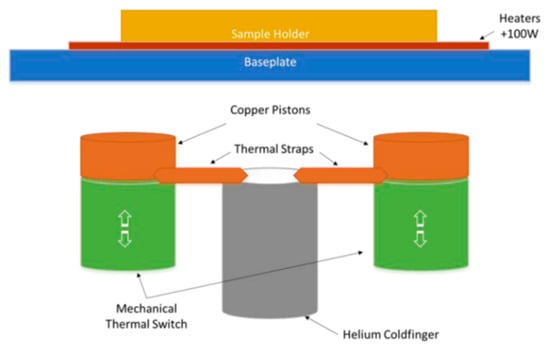
Figure 1.
Thermal vacuum cycle conceptual design.
Thermal cycling between temperatures of −150 °C and 150 °C is carried out in a vacuum chamber at a pressure below 10−6 mbar. This high temperature range is used to create accelerated aging conditions over operation conditions. This paper uses the concept of acceleration factor (AF) that is used to refer to the ratio of the acceleration characteristic between the operation level and a higher test level.
The main vacuum chamber has already been developed and is reported in [9]. The overall internal dimensions of the chamber are a 986 mm length and a 321 mm radius.
The vacuum pumping system consists of a turbomolecular vacuum pump placed in series with a rotatory pump, making it possible to maintain a pressure below 10−6 mbar inside the chamber.
3.1. Material Selection
The main criteria for material selection were thermal properties (i.e., thermal conductivity) and material costs.
Using a material with high thermal conductivity allows a heat flux higher than when using a material with low thermal conductivity. The following materials were selected to implement the instrument setup:
- Aluminum
Aluminum alloy 5083 is known for its exceptional performance in extreme environments. This alloy is a lightweight, strain-hardened, corrosion-resistant, and high-strength material that is commonly used in high-strain-rate applications such as those experienced under shock loading [10]. The properties of aluminum 5083 at 25 °C are shown in Table 1.

Table 1.
Properties of aluminum 5083 at 25 °C.
The variation in the thermal conductivity and linear expansion of aluminum 5083 [11] is shown in Figure 2.
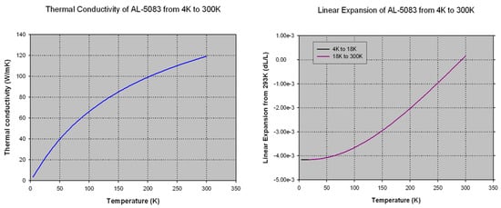
Figure 2.
Variation in the thermal conductivity and linear expansion of aluminum 5083 [11].
- Stainless steel
Austenitic stainless steels are the most common choice for high-vacuum and ultra-high-vacuum systems. Stainless steel 304 is a typical choice, and properties of stainless steel at 25 °C are shown in Table 2.
Table 2.
Properties of stainless steel at 25 °C.
The variation in the thermal conductivity and linear expansion of stainless steel 304 [11] is shown in Figure 3.
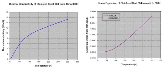
Figure 3.
Variation in the thermal conductivity and linear expansion of stainless steel 304 [11].
- Copper
Oxygen-free high-thermal-conductivity (OFHC) copper with high purity, 99.99%, is widely used in cryogenics. It is a good heat exchanger due to its good thermal conductivity and is used in the system’s thermal straps and where they are attached, namely the cold finger and pistons. The properties of copper at 25 °C are shown in Table 3.
Table 3.
Properties of copper at 25 °C.
- Epoxy
ISOVAL FR4-HF is a halogen-free epoxy glass laminate with a limiting temperature of 180 °C. Epoxy glass laminates are even usable for cryogenic applications at temperatures close to absolute zero. These laminates have increased mechanical strength and a modulus of elasticity can be observed, but at very low temperatures, for example, in liquid nitrogen or liquid helium, they do not show vitreous embrittlement like rubber or thermoplastics.
The properties of the ISOVAL FR4-HF epoxy at 25 °C are shown in Table 4.
Table 4.
Properties of the ISOVAL FR4-HF epoxy at 25 °C.
The variation in the thermal conductivity of the ISOVAL epoxy [12] is shown in Figure 4.
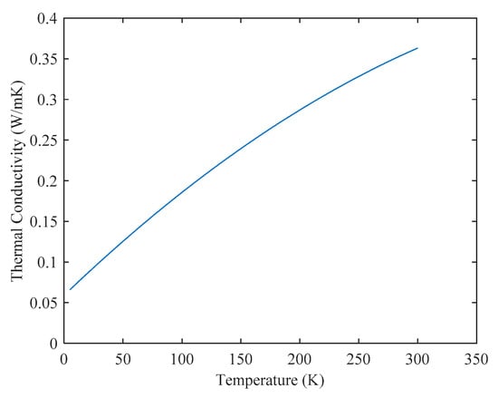
Figure 4.
Variation in the thermal conductivity of the ISOVAL epoxy [12].
3.2. Thermal Modeling
In this subsection, the thermal analysis of the chosen architecture, using both an analytical lumped circuit and the numerical finite element method, is presented.
- Approximated lumped network analysis
A simplified scheme of the thermal system is shown in Figure 5. As a rough approximation, the thermal contact resistance between the sample holder and the pistons is not considered; however, the heat flux is defined by the area and length of the copper part of the pistons. The thermal straps also add resistance to the heat flux.
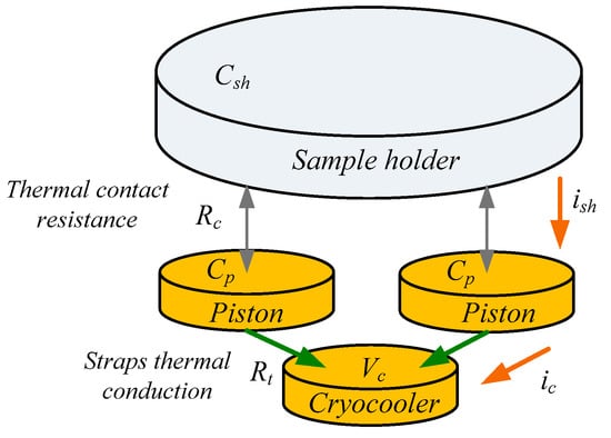
Figure 5.
Simplified scheme of the thermal system for lumped network analysis.
As a convention, heat flows from the sample holder (at a higher temperature) to the cryocooler (at a lower temperature).
Here, Vc is the temperature in the cryocooler at the generator terminals G (Figure 6), Rt is the sum of the internal resistance of the cryocooler and the thermal conduction of the copper straps, Cp is the heat capacity of the pistons, Rc is the contact resistance between the pistons and the sample holder, Csh is the heat capacity of the sample holder, ish is the heat flow between the sample holder and the pistons, and ic is the heat flow between the pistons and the cryocooler.
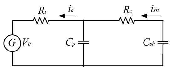
Figure 6.
Electrical transmission line equivalent circuit diagram for modeling heat conduction properties; the physical variables are specified in their thermal equivalents.
An effective way to better understand the thermal problem is to use the analogy between thermal and electrical networks. The voltage (representing the temperature) at various nodes can be calculated, together with the current (representing the heat) flow between nodes. For transient analysis, electrical capacitances (associated with thermal capacitances) are added to account for the change in the internal energy of the body with time. Thermal resistances result from geometric dimensions, thermal properties of the materials, and heat transfer coefficients [13,14].
The equivalent circuit diagram that relates the heat path from the sampler holder to the cryocooler is shown in Figure 6.
The particular solution is given by
To determine the exponential argument, e−at, the determinant must be set to zero. There are two solutions for a, given by
In Equation (8), the constants Rt and Rc were calculated as the inverse of thermal conductivity and Rt was used as the length of the section of copper straps. Rc (surface-to-surface contact coefficient) was assumed to be limited by the thermal conductivity of the copper part of the pistons. Csh was determined by the heat capacity of the sample holder, made entirely of aluminum. Cp was calculated by adding the heat capacity of the stainless steel and copper of the piston. Table 5 shows the computed constants.
Table 5.
Parameters used in the lumped model.
Replacing the constants of Table 5 in Equation (8) provides two solutions. The solutions are as follows: a→{6.979 × 10⁻¹, 1.396 × 10⁻⁴}, meaning the solutions are a linear combination of two exponential functions over time. This result was expected since there are two mechanisms involved in the cooling process, one from the thermal mass of the pistons, a very quick process, and the other from the conduction on the straps.
The lumped model provides a first approach to system dimensioning that should be complemented with a more accurate model (i.e., the finite element method).
- Finite element method
The finite element method (FEM) is the dominant discretization technique in structural mechanics. The basic concept in the physical interpretation of the FEM is the subdivision of the mathematical model into disjoint (non-overlapping) components of simple geometry, called finite elements, or elements in short. The response of each element is expressed in terms of a finite number of degrees of freedom characterized as the value of an unknown function, or functions, at a set of nodal points.
The response of the mathematical model is then considered to be approximated by that of the discrete model obtained by connecting or assembling the collection of all elements. All analyses were performed using the Simulation solution implemented using the SolidWorks framework.
For the TVC system, the main concern was thermal conductivity, either from the hot baseplate to the flange, dissipating the needed power to raise the baseplate temperatures, or from the flange to the cold baseplate. These simulations are referred to as static analyses.
A dynamic simulation was also accomplished in order to assess the time needed for a full cooldown of the system from 150 °C to −150 °C.
- FEM, static analyses
A static simulation was performed on fiberglass epoxies; these parts are the support structure of the cold pistons and sample holder. Therefore, these parts interface with extreme cold/hot parts (± 150 °C) at one extreme and the vacuum chamber at the other extreme (ambient temperature).
To assess the thermal isolation performance of these parts, static simulations in the extreme temperature range were considered as a worst-case scenario.
- Outer epoxy
The outer epoxy experiences both high and low temperatures at one end, and the other is attached to the flange, which gives a good thermal connection, so it is always at room temperature. A computer-aided design (CAD) model was used to simulate the applied thermal loads. On the baseplate, the thermal loads applied for this simulation are −150 °C and 150 °C, as shown in Figure 7.
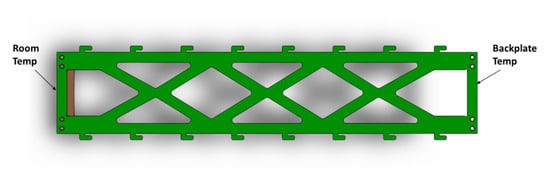
Figure 7.
3D model used to simulate the applied thermal loads. On the baseplate, the thermal loads applied for this simulation are −150 °C and 150 °C.
A mesh is a discretization of the CAD model. Finite elements and nodes define the basic geometry of the physical structure being modeled, splitting the geometry into relatively small and simple geometric entities called finite elements. Each element in the model represents a discrete portion of the physical structure, which is represented by many interconnected elements. Shared nodes connect these elements to one another.
Several mesh densities were evaluated, and the analysis results were checked to converge to a unique solution. The solution obtained from the numerical model is generally a good approximation of the solution of the physical problem being simulated. An important parameter in the assessment of mesh quality is aspect ratio checks [15]. Simulation accuracy is best achieved by a mesh with uniform-size elements whose edges are equal in length. Therefore, by definition, the aspect ratio of a perfect tetrahedral is 1.0.
Table 6 summarizes the mesh used in the simulation. Since 89% of the elements have an aspect ratio below 3.0, the mesh is considered of good quality.
Table 6.
Mesh used in the simulation.
Figure 8 shows a representation of the mesh used in the simulation.
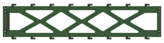
Figure 8.
Representation of the mesh used in the simulation.
In the simulations, only thermal conductivity was considered, which is a good approximation since there is no convection in vacuum and all thermal radiation from the wall of the chamber, at room temperature, is assumed to be shielded by the MLI blankets.
The simulations are driven by the heat balance equation given by
where qx, qy, and qz are the heat flux in the x, y, and z directions, Q is the internal heat generated/absorbed by the body (volume), c is the specific heat, ρ is the mass density, and T is the temperature.
Fourier’s law of heat conduction relates heat flux and temperature and is proportionality constant to k, the thermal conductivity. For an orthotropic body (volume element), with the axes of orthotropy coinciding with the coordinate axes, Fourier heat conduction is given by
Considering Equations (9) and (10), is given by
Analysis of steady-state heat conduction problems involves setting the term equal to zero and assuming Q to be independent of time.
Taking this into account, in the first simulation, the baseplate is considered at 150 °C. As shown in Figure 8, the temperature applied on the left side is the flange temperature (room temperature, 25 °C), and on the right side, 150 °C is applied.
Figure 9 shows the results of this simulation. The top plot shows the temperature gradient on the epoxy, and on the bottom the heat flux. The important result here is the total power transferred through the epoxy, which should be the minimum. The simulation shows 0.02 W being transferred.
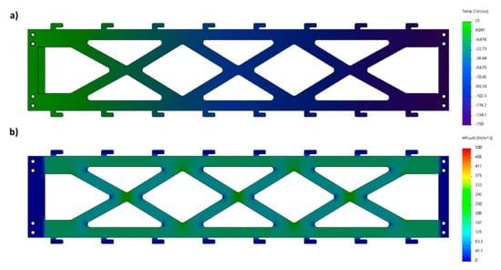
Figure 9.
Thermal analysis of the outer epoxy support when the large clutch is at −150 °C. (a) A temperature map and (b) the heat flux. The power transferred in this simulation was about 0.02 W.
Since the model is the same, the same mesh was used to simulate it with a different temperature in the extremity; the result is as plotted below. Again, the top of Figure 10 shows the temperature gradient on the epoxy, and on the bottom the heat flux. The power transferred was 0.015 W.
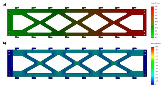
Figure 10.
Thermal analysis of the outer epoxy support when the large clutch is at 150 °C. (a) A temperature map and (b) the heat flux. The power transferred in this simulation was about 0.015 W.
We concluded that these parts are a good solution for thermal isolation and stiff enough for mechanical support.
- FEM, dynamic simulations
Dynamic simulations were performed to assess the time needed for cooldown during a thermal cycle. A simplified CAD model used in the dynamic simulation. Figure 11 shows the CAD model used in the dynamic simulation. The output power of the cryocooler depends on its temperature, and that dependency was used in the simulation, with the baseplate set to 150 °C as the initial temperature. The results of this dynamic simulation are shown in Figure 12.
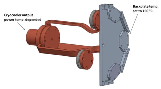
Figure 11.
CAD model used in the dynamic simulation.
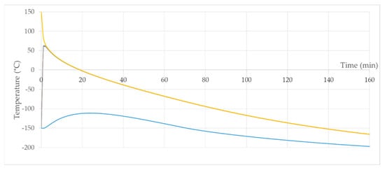
Figure 12.
Cooldown time simulation.
A cooldown rate of 4 ℃/min in the 150 ℃ to −150 ℃ range can be measured from Figure 13. The blue line represents the temperature of the cold finger, and the others represents three sensors placed on the top of the sample holder. It is possible to see that the sample holder can reach a temperature of −150 ℃ in 135 min.
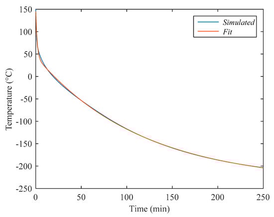
Figure 13.
Cooldown fit.
To compare this result with the one obtained from the lumped model, it was necessary to perform a non-linear fitting of the temperature of the sample holder. A two-phase exponential decay function with a time constant parameter model was used. The function for the two-phase exponential decay is given by
The cooldown fit is shown in Figure 13.
For the fit of the temperature of the sample holder over time, it is possible to determine two time constant parameters, A1 and A2. Table 7 shows the parameters calculated.
Table 7.
Parameters determined for the fit of the dynamic simulation result.
3.3. Thermal Expansion
This is only a brief discussion of thermal expansion since it does not play a major role in this system. Even with the temperature ranges expected for this system, the expansion was in the order of a few micrometers. For instance, the expanse of stainless steel in the parallelepiped was 0.135 mm and in the epoxy was 0.266 mm. This means that alignment pins are not an option, but the use of screws is acceptable.
3.4. Mechanical Design
A 3D CAD model is presented in Figure 14.
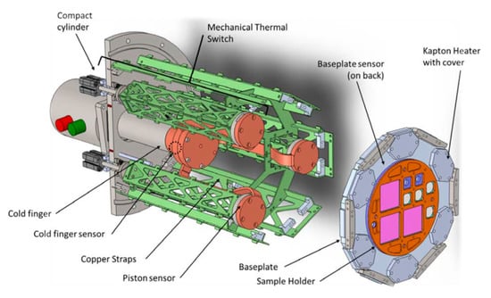
Figure 14.
Thermal vacuum cycle mechanical CAD design.
In Figure 14, the main parts are identified as follows:
- (1)
- Thermal-mechanical switch
Mechanical switches consist of a compressed-air pneumatic system using a flexible bellow as a linear vacuum feedthrough. The cold part is isolated by an epoxy with low thermal conductivity, used in cryogenics and vacuum applications. This system allows one to disconnect the cold source from the hot source mechanically.
- (2)
- Baseplate
The baseplate is the part of the system where the resistors are attached, and the thermal connection with the cold finger is made on its back. The samples to be tested will be placed on this part.
- (3)
- Heater
For the heater, we selected Kapton flexible foils [9] because they have a wide operational temperature and we have used them in the past for this kind of application. Kapton foil heaters are positioned between the sample holder and the baseplate.
- (4)
- Cold finger (heat pump)
A helium cryocooler is used to cool down the baseplate. The cryocooler, at −150 ℃, can transfer 90 W. The section area of the copper strip can be customized to fit the desired power flux.
- (5)
- Thermal isolation
Besides the isolation provided by the epoxies, an MLI blanket at room temperature is used to shield from the radiation emitted by the chamber walls.
3.5. Operation and Control
To fulfil European Space Agency (ESA) standard requirements, for TVC, there are four stages of operation: warm-up, high-temperature dwelling (HTD), cooldown, and low-temperature dwelling (LTD). Temperature control is achieved by:
- (a)
- Monitoring the sample holder with PT100 temperature sensors; due to low voltage measurements, Omega controllers [16] are used.
- (b)
- Heating procedure:
- (i)
- During heating, the thermal switch thermally disconnects the cold finger from the baseplate.
- (ii)
- Kapton resistors are tuned on until achievement of the highest temperature (e.g., 150 °C).
- (c)
- During cooldown:
- (iii)
- The resistors are turned off and the thermal-mechanical switches are turned on, thermally connecting the cold finger to the baseplate. This situation endures up to the minimum temperatures (e.g., −150 °C).
- (iv)
- Temperature stabilization turns on the resistors.
4. Prototype Implementation
After the design, we performed part procurement and in-house manufacture. The manufacture processes are described as well as the assembly process.
4.1. Manufacture
All aluminum and epoxy parts were produced in the Department of Physics, Sciences Faculty, University of Lisbon workshop using a 3D milling machine. The epoxy after the CNC (computer numerical control) milling process is shown in Figure 15a; the display of most parts produced using the CNC machine at the workshop is shown in Figure 15b.
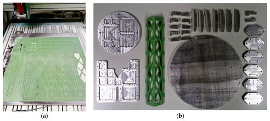
Figure 15.
(a) Epoxy after the CNC milling process. (b) Display of most parts produced using the CNC machine during the workshop.
4.2. Integration
The TVC setup was assembled in a cylindrical vacuum chamber. Figure 16a–d shows the assembly process in detail [12].
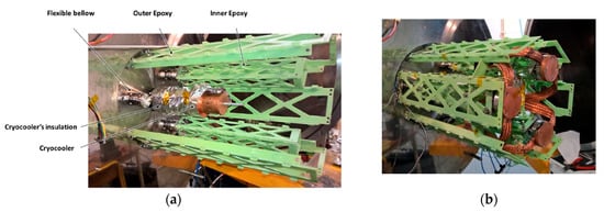
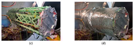
Figure 16.
(a) Assembly of the outer epoxy, showing details of the thermal-mechanical switch (flexible bellow and inner epoxy). (b) System without the aluminum baseplate, showing the copper thermal interface of the pistons. (c) System with the aluminum baseplate. (d) System with the aluminum baseplate and MLI [12].
4.3. Data Acquisition and Control
Data acquisition and control for thermal cycling were performed by the LabVIEW program using a DAQ (Data acquisition system) from LabJack and a SERIAL protocol.
LabJack U12 is a USB-based measurement and automation peripheral. It has eight analogue input signals, which can operate as eight single-ended channels or four differential channels. Each input has a 12-bit resolution, and the input range for a single-ended measurement is ±10 V.
Due to the need for nine digital output pins and an analogue voltage reader, LabJack U12 was chosen as the control unit to completely monitor and control the thermal cycles in this project.
4.4. Heaters
The heater chosen was a patch heater, which consists of an electrical resistance element between two flexible insulating materials, such as Kapton. The one used for this project was a Kapton heater from OMEGA Engineering (model number KHLV-102/10) [17].
Due to the high temperatures achieved, a patch heater without PSA (pressure sensitive adhesive) tape must be used. Therefore, there is a need to use a fixation method that uses small aluminum caps. In Figure 17, a patch heater is attached to the aluminum cap before installation.
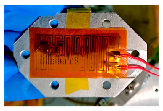
Figure 17.
Omega patch heater attached by thermal fixation before installation.
This patch heater has a size of 3 × 5 cm2 and operates at 28 V with a power of 20 W. A total of six heaters were installed, with a combined power of 120 W; each heater could be controlled independently through the control board in order to allow fine control of the baseplate temperature.
4.5. Thermal-Mechanical Switch Control
Mechanical switches use air-operated cylinders to create a linear movement. The air compact cylinder option was chosen over, for example, a stepper motor because to achieve good thermal contact, high pressure is needed (as well as surface roughness, waviness, and flatness on the contact surfaces). Therefore, the controlled variable is the pressure and not the position. There are three mechanical switches in the TVC system; each one is composed of a compact cylinder and a solenoid valve.
4.6. Control Board
Digital signals from the control unit (LabJack U12) needed to be converted to the operating voltage of the heat resistors and pneumatics. In addition, solid-state relays were used to electrically isolate the circuits.
To control the pneumatics driver, a low-current and dual-channel solid-state relay was used—Avago ASSR-1228. In addition, for driving heat resistors, VO14642AT from Vishay Semiconductors was used, providing a maximum load of up to 2 A in DC.
Envisaging independent control of heating resistors and pneumatics, six solid-state relays from Vishay Semiconductors and two from Avago were used, respectively.
4.7. Temperature Acquisition
A PT100 platinum resistance thermometer was used instead of a standard temperature sensor, such as LM35, due to the low temperatures reached in a normal thermal cycle. Platinum resistance thermometers offer excellent accuracy over a wide temperature range from −200 °C to +650 °C. For a PT100 sensor, a 1 °C temperature change causes a 0.384 Ω change in resistance, so even a small error in measurement of the resistance (for example, the resistance of the wires leading to the sensor) can cause a large error in the temperature measurement. For precision, a four-wire scheme is usually used to carry the sense current and a two-wire scheme to measure the voltage across the sensor element.
CN7800, from OMEGA Engineering Inc., was used as an off-the-shelf temperature monitor since it measures the PT100 resistor using the four wires.
4.8. Cryocooler
The cryocooler used was from Advanced Research Systems (ARS), with an ARS-4HW compressor and a DE-104(T) cold head. The cooling capacity of the cryocooler was temperature dependent, as shown in Figure 18.
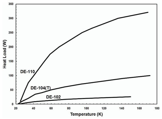
Figure 18.
Cryocooler cooling capacity.
During the thermal cycles, the heat load on the cold head goes from about 40 W, when the temperature at the clod head is the minimum (around 60 K), to 70 W at a maximum temperature of about 115 K.
4.9. User LabVIEW Interface
The user interface was developed in LabVIEW to display the information gathered from the sensors mentioned above and the status of the actuators, i.e., the patch heaters and pneumatic actuators. Figure 19 shows a complete view of the control panel [12].
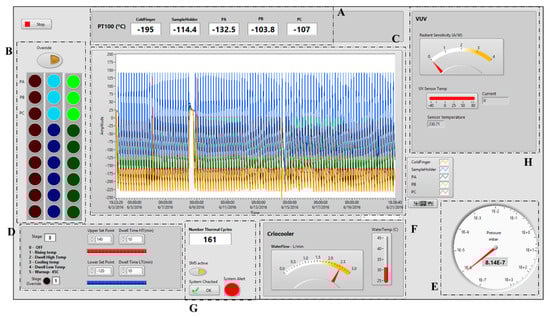
Figure 19.
Interface of the control panel.
- This panel displays the current temperature in each of the five PT100 sensors installed.
- Actuators’ control panel. This panel consists of an Override button and a matrix of buttons that allows one to control and know the state (ON/OFF) of an actuator. The matrix is divided into three columns: the first with red buttons, the second with blue buttons, and the third with green ones, representing, respectively:
- User manual input that can override the automatic control if the Override button is toggled ON
- Automatic control input
- The state of the output to the control board
- Displays the temperature over time.
- Stage control panel. As mentioned before, there are four stages in a normal thermal cycle, although due to functionality reasons, two more were added: an OFF stage, where all automatic controls are disabled, and a warm-up stage (up to −45 °C), which is used to ensure a secure temperature for opening the system without the formation of ice inside the chamber. These two stages are only assessable through the Stage Override button. In this panel, it is also possible to define the upper and lower temperature limits, as well as the dwelling times for each one individually.
- Displays the current pressure inside the chamber.
- Displays the data captured from the cryocooler and cryocooler monitor.
- System alert panel. This advises the user on whether some parameters, i.e., the cryocooler temperature, water flow, cold-finger temperature, and vacuum pressure, are outside normal values. This warning is represented by the red light present in this panel, as well by sending a text message to a pre-defined cell phone number, and it also displays the number of cycles already done.
- Reading from an ultraviolet (UV) sensor.
5. Experimental Methods and Results
After the setup was developed, it was calibrated and tested.
The cool-out time from 150 °C to −150 °C was about 3 h 40 min [1], while the simulated time was 2 h 5 min (see Figure 12). The main reasons for these differences were losses by radiation and other conduction losses (e.g., losses through electric wires) that were not considered in the FEM model. The reason to not consider radiation losses was that the system was shielded by MLI during operation (Figure 16d). The MLI minimizes radiation losses but does not eliminate them totally.
After calibration, a sample test campaign was performed [2]. In this section, some results of the sample test campaign are reported. MLI debris generated after ATOX exposure and paint flaking, which occurred after the full test campaign, are presented and discussed.
5.1. MLI Debris Generation after ATOX Exposure
During ATOX exposure, a sample tray was positioned below the sample holder (to catch debris); see Figure 20. Each tray was analyzed with scanning electron microscope (SEM)-based energy-dispersive X-ray spectrometry (EDX). Figure 20 depicts the position of the sample trays (in relation to the sample holder). Three sample trays were positioned below the sample holder; each sample tray was a silicon wafer.
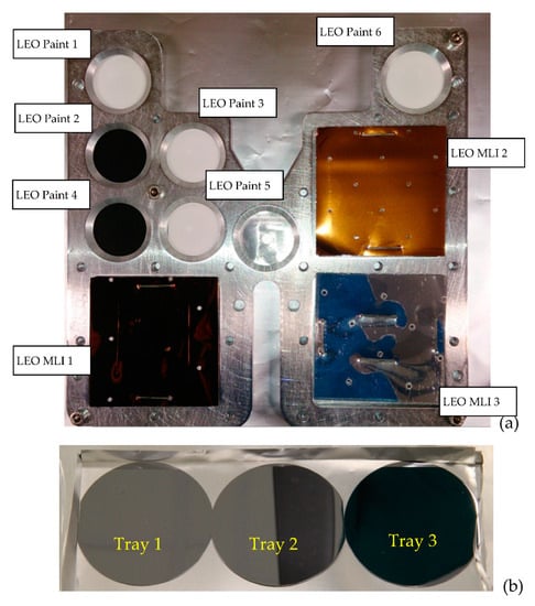
Figure 20.
(a) ATOX (atomic oxygen) sample holder. (b) Silicon sample trays.
In the case studies, four types of images are presented, namely SEM images, EDX layer image, EDX single-element image, and EDX-detected spectrum. Examples of these images are presented in Figure 21.
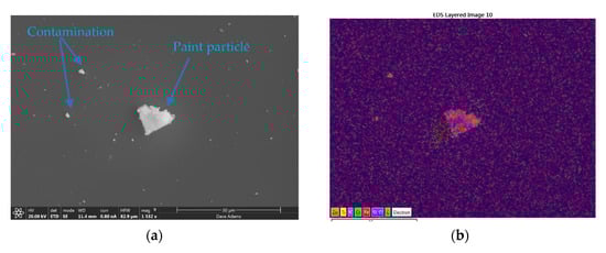
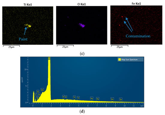
Figure 21.
Examples in case studies. (a) SEM image, (b) EDX layer image, (c) EDX single-element image, and (d) EDX spectrum.
By analyzing individual particles’ compositions, one can identify what the contamination is from the ATOX system (generation of iron particles by laser ablation) and what samples originate from particles/fibers.
Table 8 presents LEO sample paints’ compositions.
Table 8.
LEO sample paints’ compositions.
Table 9 shows the LOE ATOX particle size or fiber length (taken from SEM analysis) and origin identification.
Table 9.
LEO ATOX particle size or fiber length and origin identification.
5.2. Paint Flaking after Full Test
The full test campaign specifications are described in [2]. After the full test campaign, ATOX (in ESTEC) [18], TVC, and VUV exposure (in the developed setup) [1], the samples were visually inspected under a microscope. Some evidence of flaking in PSB paint from MAP on a CFRP (carbon fiber-reinforced polymer) substrate is shown in Figure 22.
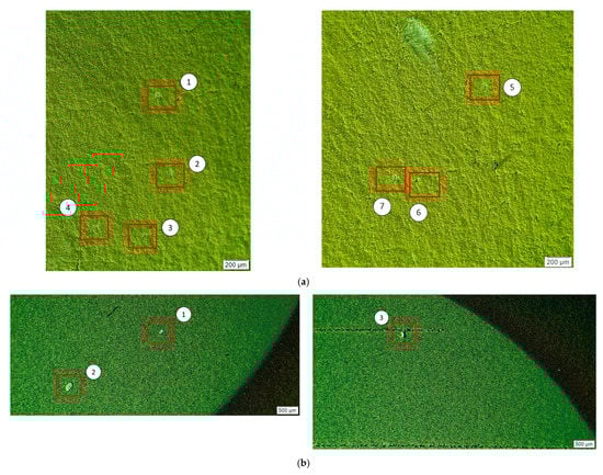
Figure 22.
Flaking evidence: (a) PSB on CFRP-detected flaking. (b) PUK on aluminum.
Table 10 shows the area of the flakes in both paints, i.e., PSB on CFRP and PUK on aluminum.
Table 10.
Area of the flakes in both paints.
6. Conclusions
In this paper, we reported the development of a cryogenic test setup that can expose material samples to a simulated space environment (TVC and VUV exposure). The development approach consisted of the implementation of an innovative architecture that make uses of a He cryocooler. For successful development of the setup, the selection of materials and iterative thermal and mechanical simulations were considered critical. The developed setup can provide VUV exposure (sun radiation simulation) and thermal vacuum cycling at ±150 °C. This paper is a continuation of a previous work. The setup was developed and used in the framework of the ESA project Space Debris from Spacecraft Degradation Products to test material samples during a long period (i.e., simulating satellites’ external material exposure beyond the satellite life). Within the ESA project, the materials were first exposed to ATOX at ESTEC and then subjected to tests in the developed setup. MLI debris generation was evaluated after ATOX exposure, and paint flaking was evaluated after the full test campaign. The tests resulted in the observation of micron-size debris from the MLI and from the paint samples.
Author Contributions
Creation and development of the proposed circuit, T.F.; analysis and validation, P.G.; and analysis and proofreading, P.G., R.M. and A.A. The other parameters were decided by the authors in a mutual way. All authors have read and agreed to the published version of the manuscript.
Funding
There was no external funding, and all costs were borne by the authors.
Institutional Review Board Statement
Not applicable.
Informed Consent Statement
Not applicable.
Data Availability Statement
The study did not report any data.
Acknowledgments
This research received no external funding. The ongoing work presented in this paper was performed under ESA contract 4000113047/14/NL/LF/TU-IAS, Space Debris from Spacecraft Degradation Products; the Foundation for Science and Technology (FCT), through the CENTRA project UIDB/00099/2020; the Foundation for Science and Technology (FCT) under the LAETA project UIDB/50022/2020; the Foundation for Science and Technology (FCT) under the Institute of Earth Sciences (ICT) project UIDB/04683/2020.
Conflicts of Interest
The authors declare no conflict of interest.
Nomenclature
| AF | Acceleration factor |
| ARS | Advanced research systems |
| ATOX | Atomic oxygen |
| CAD | Computer-aided design |
| CFRP | Carbon fiber-reinforced polymer |
| CNC | Computer numerical control |
| EDX | Energy-dispersive X-ray spectrometry |
| ESA | European Space Agency |
| ESTEC | European Space Research and Technology Centre |
| FEM | Finite element method |
| HEX | Hexadecimal |
| HTD | High-temperature dwelling |
| LEO | Low Earth orbit |
| LTD | Low-temperature dwelling |
| MAP | European space paints supplier |
| MLI | Multilayer insulation |
| OFHC | Oxygen-free high thermal conductivity |
| PSA | Pressure-sensitive adhesive |
| PSB/PUK | Thermal control coatings for satellites |
| PTC | Positive temperature coefficient |
| SEM | Scanning electron microscope |
| TO | Thermal optical properties |
| TVC | Thermal vacuum cycling |
| UV | Ultraviolet |
| VDA | Vacuum-deposited aluminum |
| VUV | Vacuum ultraviolet |
References
- Gordo, P.; Frederico, T.; Melicio, R.; Duzellier, S.; Amorim, A. System for space materials evaluation in LEO environment. Adv. Space Res. 2020, 66, 307–320. [Google Scholar] [CrossRef]
- Shan, M.; Guo, J.; Gill, E. Review and comparison of active space debris capturing and removal methods. Prog. Aerosp. Sci. 2016, 80, 18–32. [Google Scholar] [CrossRef]
- Rowe, D.M.; Bhandari, C.M. Modern Thermoelectrics; Reston Publishing Company: Reston, VA, USA, 1983. [Google Scholar]
- Advanced Cooling Technologies. Operating Temperature Range: Working Fluids Theoretically Operate from the Triple Point to the Critical Point. Available online: https://www.1-act.com/operating-temperature-range/ (accessed on 3 December 2020).
- Dietrich, M.; Euler, A.; Thummes, G. Compact thermal heat switch for cryogenic space applications operating near 100 K. Cryogenics 2014, 59, 70–75. [Google Scholar] [CrossRef][Green Version]
- Rongong, J.A.; Goruppa, A.A.; Buravalla, V.R.; Tomlinson, G.R.; Jones, F.R. Plasma deposition of constrained layer damping coatings. Proc. Inst. Mech. Eng. Part C J. Mech. Eng. Sci. 2004, 218, 669–680. [Google Scholar] [CrossRef]
- Yu, L.; Ma, Y.; Zhou, C.; Xu, H. Damping efficiency of the coating structure. Int. J. Solids Struct. 2005, 42, 3045–3058. [Google Scholar] [CrossRef]
- Catania, G.; Strozzi, M. Damping oriented design of thin-walled mechanical components by means of multi-layer coating technology. Coatings 2018, 8, 73. [Google Scholar] [CrossRef]
- Sousa, P.C. A Infra-Estrutura de Teste da Câmara Multi-Telescópio do Gravity. Master’s Thesis, Faculdade de Ciências, Universidade de Lisboa, Lisboa, Portugal, 2012. [Google Scholar]
- KwonJ, J.B.; Huh, J.; Huh, H.; Kim, J.S. Micro-tensile tests of aluminum thin foil with the variation of strain rate. Dyn. Behav. Mater. 2012, 1, 89–100. [Google Scholar]
- NIST Cryogenic Materials Property Database. Cryogenic Technology Group at NIST. Available online: https://www.nist.gov/publications/cryogenic-technologies-group-website (accessed on 3 December 2020).
- Frederico, T. Development of a Cryogenic Facility for the Generation of Space Debris. Master’s Thesis, Faculdade de Ciências, Universidade de Lisboa, Lisboa, Portugal, 2017. [Google Scholar]
- Tilmans, H.A.C. Equivalent circuit representation of electromechanical transducers: I. Lumped-parameter systems. J. Micromech. Microeng. 1996, 6, 157–176. [Google Scholar] [CrossRef]
- D’Azzo, J.J.; Houpis, C.H. Linear Control Systems Analysis and Design with MATLAB; CRC Press: Boca Raton, FL, USA, 2013; p. 6e. [Google Scholar]
- Abbey, T. Accuracy and Checking in FEA, Part 1. Available online: https://www.digitalengineering247.com/article/accuracy-and-checking-in-fea-part-1 (accessed on 3 December 2020).
- Omega Company. Available online: https://www.omega.co.uk/pptst/CN7800.html (accessed on 3 December 2020).
- Insulated Flexible Kapton Heaters. Available online: https://www.omega.nl/pptst/KHR_KHLV_KH.html (accessed on 3 December 2020).
- Graham, C.B.; Roberts, G.T.; Chambers, A.R. Measurement of 5-eV atomic oxygen using carbon based films: Preliminary results. IEEE Sens. J. 2005, 5, 1206–1213. [Google Scholar]


Publisher’s Note: MDPI stays neutral with regard to jurisdictional claims in published maps and institutional affiliations. |
© 2021 by the authors. Licensee MDPI, Basel, Switzerland. This article is an open access article distributed under the terms and conditions of the Creative Commons Attribution (CC BY) license (http://creativecommons.org/licenses/by/4.0/).